Wave-packet dynamics of an atomic ion in a Paul trap: approximations and stability

Abstract

Using numerical simulations of the time-dependent Schrödinger equation, we study the full quantum dynamics of the motion of an atomic ion in a linear Paul trap. Such a trap is based on a time-varying, periodic electric field, and hence corresponds to a time-dependent potential for the ion, which we model exactly. We compare the center of mass motion with that obtained from classical equations of motion, as well as to results based on a time-independent effective potential. We also study the oscillations of the width of the ion’s wave packet, including close to the border between stable (bounded) and unstable (unbounded) trajectories. Our results confirm that the center-of-mass motion always follow the classical trajectory, that the width of the wave packet is bounded for trapping within the stability region, and therefore that the classical trapping criterion are fully applicable to quantum motion.

PACS Nos.: 37.10.Ty, 02.60.Cb

1 Introduction

A Paul trap consists of a series of electrodes creating a time-dependent (radio-frequency) electric field that enables the trapping of charged particles (specifically ions).[1, 2, 3] In its linear configuration,[4, 5] it provides the capacity of trapping many ions simultaneously along an axis. The linear Paul trap is suitably designed for quantum computing experiments, reducing the Coulomb repulsion between the ions at the center of the trapping region, reducing a possible increase in amplitude of the micromotion of the ion.[4] Also, the spacing between electrodes and spacing between ions provide a good environment for laser controlling experiments.[6]

The difficulty of a numerical treatment of the quantum dynamics of a trapped ion stems from the fact that the trapping potential is time dependent, on a time scale that can be considered slow with respect to the internal dynamics of the ion, and that the motion of the center of mass and the width of the wave function can cover greater than micrometer-sized regions. Wave packet dynamics of trapped ions require thus large spatial grids and long simulation times. Consequently, numerical simulations of the ion motion in the trap have mostly been limited to classical trajectories (see, e.g., Refs. Brkic_PRA_2006,Dawson_JVST_1968,Lunney_JAP_1989,Londry_JASMS_1993,Reiser_IJMSIP_1992,Wu_JASMS_2006,Wu_IJMS_2007,Herbane_IJMS_2011,Cetina_PRL_2012), or have rested on the effective potential approximation,[15] treating the trapping potential as purely harmonic (see, e.g., Refs. Gardiner_PRA_1997,Zheng_PLA_1998,Moya-Cessa_PR_2012). There have been only limited studies of the quantum dynamics with the full time-dependent potential, either looking at the breathing of a wave packet in the center of the trap,[19] or comparisons between quantum trajectories and an effective potential approximation.[3] While there exists what can be called analytical solutions for the center-of-mass motion or the width of the wave packet,[20, 21, 22, 23, 24, 19] simulations based on these formulas must ultimately rely on involved numerical calculations. One notable exception is an approximate solution for a breathing wave packet,[24] which we will address below.

In this paper, we present a full investigation of the quantum-mechanical motion of an atomic ion in a linear Paul trap, using the actual time-dependent trapping potential, using numerical simulations of the spatial wave packet dynamics, focusing our attention on both the trajectory of the center of mass and the width of the wave packet. We compare our results with classical simulations of the ion motion and examine the validity of the effective potential approximation. We also look at the applicability of classical trapping stability criteria to quantum motion. Indeed, while a Floquet analysis[20, 21] and the study of Ref. Li_PRA_1993 point to the applicability of the classical criteria in all cases, Wang et al.[25] have claimed that there are trapping parameters for which a quantum trajectory is stable, while the classical counterpart would not be.

This paper is arranged as follows. We start by presenting the models, quantum and classical, for the dynamics of an atomic ion in a linear Paul trap. The numerical methods corresponding to both models are presented in Sec. 3. This is followed by the results of the various simulations. Finally, concluding remarks are given in Sec. 5.

2 Model for an atomic ion in a linear Paul trap

2.1 Hamiltonian of an atomic ion in a linear Paul trap

We consider a linear Paul trap, such as the one described in Refs. Berkeland_JAP_1998,Berkeland_PRL_1998,Rohde_JOB_2001, constructed of four cylindrical electrodes, each located at the corner of a square. A pair of electrodes that are opposing each other diagonally is attached to a radio-frequency source and the other pair is grounded. Also, in order to confine ions inside the trapping device, a static potential is applied to two ring-shaped electrodes, located near the end of the cylindrical electrodes. The time-dependent electric potential near the center of a linear Paul trap is given by

$$\Phi(t)=\Phi_{\mathrm{rf}}(t)+\Phi_{\mathrm{s}},$$ (1)

where $\Phi_{\mathrm{rf}}(t)$ is a quadrupolar, time-dependent electric potential of the form

$$\Phi_{\mathrm{rf}}(t)=\frac{1}{2}\frac{V_{0}}{r_{0}^{2}}\left(x^{2}-y^{2}\right)\cos\Omega t,$$ (2)

with $V_{0}$ is the amplitude of the radio-frequency potential of frequency $\Omega$ and $r_{0}$ is the minimum distance from the electrodes to the central (trap) axis.

The form of the static potential is dependent on the configuration of the system, but it is approximated to have a quadratic dependence on spatial coordinates, especially in the region close to the trapping axis,[5, 26] leading to

$$\Phi_{\mathrm{s}}=\frac{\kappa U_{0}}{z_{0}^{2}}\left[z^{2}-\frac{1}{2}\left(x^{2}+y^{2}\right)\right],$$ (3)

in which $U_{0}$ is the amplitude of the static potential, $\kappa$ is the geometric factor which is a parameter that can be found experimentally from the oscillation frequency of an ion in the trap,[5] and $z_{0}$ is half the distance between ring-shaped electrodes, along the trapping axis.

Now considering an atomic ion in such an external trapping field, we have the Hamiltonian for the motion of the ion as

$$\hat{H}=-\frac{\hbar^{2}}{2m}\nabla_{\mathbf{r}}^{2}+Ze\Phi,$$ (4)

where $m$ is the mass of the ion with charge $Z$, $\mathbf{r}$ its position vector, $\hbar$ the reduced Planck constant, and $e$ the elementary charge.

2.2 Classical trajectories and stability conditions

From the Hamiltonian of the system for an ion in a linear Paul trap, we can find the classical trajectories of the motion of the center of mass. Using the standard approach,[2, 3, 29] we write the classical equation of motion of an ion in a linear Paul trap as

$$m\ddot{\mathbf{r}}+Ze\vec{\nabla}\Phi=0$$ (5)

and rewriting it explicitly in its components

$$m\ddot{x}+Ze\left[-\frac{\kappa U_{0}}{z_{0}^{2}}+\frac{V_{0}}{r_{0}^{2}}\cos\Omega t\right]x =0,$$ (6a)

$$m\ddot{y}+Ze\left[-\frac{\kappa U_{0}}{z_{0}^{2}}-\frac{V_{0}}{r_{0}^{2}}\cos\Omega t\right]y =0,$$ (6b)

$$m\ddot{z}+Ze\left[\frac{2\kappa U_{0}}{z_{0}^{2}}\right]z =0,$$ (6c)

we obtain the Mathieu equation

$$\frac{\mathrm{d}^{2}\mathbf{r}}{\mathrm{d}\tau^{2}}+(a-2q\cos 2\tau)\mathbf{r}=0,$$ (7)

by setting $\tau=\Omega t/2$ and

$$a_{x}=a_{y} =-\frac{4Ze}{m\Omega^{2}}\frac{\kappa U_{0}}{z_{0}^{2}},$$ (8a)

$$a_{z} =\frac{8Ze}{m\Omega^{2}}\frac{\kappa U_{0}}{z_{0}^{2}},$$ (8b)

$$q_{x}=-q_{y} =-\frac{2Ze}{m\Omega^{2}}\frac{V_{0}}{r_{0}^{2}},$$ (8c)

$$q_{z} =0\,.$$ (8d)

Stable solutions of the Mathieu equation, corresponding to a trapped ion, exist for certain regions in the $a$–$q$ plane.[30] We will consider potential values $U_{0}$ and $V_{0}$ close to the so-called first stability region, illustrated in Fig. 1.

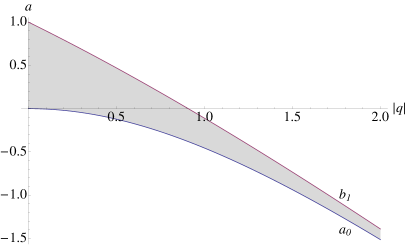
Figure 1: (Color online) Left panel: First stability region of the Mathieu equation (7), bounded by the characteristic values $a_{0}$ and $b_{1}$,[30] for motion in the xy plane. Right panel: Stability diagram of a linear Paul trap for the full 3D motion for a Ca⁺ ion. In both panels the shaded region corresponds to stable trajectories.

2.3 Effective potential approximation

The bounded solutions to the ion motion, Sec. 2.2, are periodic and consist of two types of motions, an average secular motion on which a high-frequency micromotion is superposed.[2, 3] The secular motion corresponds to the trajectory which should be observed in the time-average electric potential and the small-amplitude micromotion is driven at the frequency of the oscillation of the potential. As the time-dependent trapping field gives rise to approximately harmonic secular motion of a particle in all directions,[24] specifically near the center of the trap,[5] the problem can be approximated using a harmonic oscillator potential.[3, 15] This approximation is called effective potential approximation or adiabatic approximation, and is used to calculate an approximated wave function,[3] which can be compared to the actual wave function.

The equation of the motion for the ion can be written as[3]

$$m\ddot{\mathbf{r}}=\mathbf{F}_{\mathrm{sm}}(\mathbf{r})+\mathbf{F}_{\mathrm{mm}}(\mathbf{r},t),$$ (9)

where $\mathbf{F}_{\mathrm{sm}}$ and $\mathbf{F}_{\mathrm{mm}}$ are the forces responsible for the secular motion and the micromotion, respectively. Decomposing the acceleration as $\ddot{\mathbf{r}}=\ddot{\mathbf{r}}_{\mathrm{sm}}+\ddot{\mathbf{r}}_{\mathrm{mm}}$, the micromotion being purely caused by the time-dependent part of the potential, we have

$$m\ddot{\mathbf{r}}_{\mathrm{mm}}=-Ze\nabla_{\mathbf{r}}\Phi_{\mathrm{rf}}(\mathbf{r},t).$$ (10)

The equation of motion (9) becomes, after expansion to first order in $\mathbf{r}_{\mathrm{mm}}$ around $\mathbf{r}_{\mathrm{sm}}$,

$$m(\ddot{\mathbf{r}}_{\mathrm{sm}}+\ddot{\mathbf{r}}_{\mathrm{mm}}) =\mathbf{F}_{\mathrm{sm}}(\mathbf{r}_{\mathrm{sm}})+\mathbf{F}_{\mathrm{mm}}(\mathbf{r}_{\mathrm{sm}},t)$$

$$\quad+\mathbf{r}_{\mathrm{mm}}\left(\left.\nabla_{\mathbf{r}}\mathbf{F}_{\mathrm{sm}}(\mathbf{r})\right|_{\mathbf{r}=\mathbf{r}_{\mathrm{sm}}}+\left.\nabla_{\mathbf{r}}\mathbf{F}_{\mathrm{mm}}(\mathbf{r},t)\right|_{\mathbf{r}=\mathbf{r}_{\mathrm{sm}}}\right)$$ (11)

We now average Eq. (11) over one period of the micromotion, $\left(2\pi/\Omega\right)$, and, using Eq. (10), we get the effective potential energy for the time-dependent part of the potential,[3]

$$V_{\mathrm{eff},\mathrm{rf}} =\left\langle\frac{\left[\nabla_{\mathbf{r}}\Phi_{\mathrm{rf}}(\mathbf{r})\right]^{2}}{2m}\right\rangle$$

$$=\frac{1}{4m}\left(\frac{ZeV_{0}}{\Omega r_{0}^{2}}\right)^{2}\left(x^{2}+y^{2}\right)$$ (12)

and, consequently, the total effective potential energy is obtained as

$$V_{\mathrm{eff}}(\mathbf{r}) =Ze\Phi_{\mathrm{s}}+V_{\mathrm{eff},\mathrm{rf}}$$

$$=\left[\frac{1}{4m}\left(\frac{ZeV_{0}}{\Omega r_{0}^{2}}\right)^{2}-\frac{Ze\kappa U_{0}}{2z_{0}^{2}}\right]\left(x^{2}+y^{2}\right)+\frac{Ze\kappa U_{0}}{z_{0}^{2}}z^{2},$$ (13)

corresponding to a harmonic oscillator with frequencies

$$\omega_{x}^{2}=\omega_{y}^{2} =\left(\frac{ZeV_{0}}{\sqrt{2}m\Omega r_{0}^{2}}\right)^{2}-\frac{Ze\kappa U_{0}}{mz_{0}^{2}},$$ (14a)

$$\omega_{z}^{2} =\frac{2Ze\kappa U_{0}}{mz_{0}^{2}}.$$ (14b)

2.4 Floquet representation

Since the only time dependence in the Hamiltonian (4) is periodic with period $\Omega$, see Eq. (2), it is possible, using Floquet’s theorem, to rewrite the solutions in terms of an effective time-independent Hamiltonian.[31] In the case at hand, this can lead to an analytical representation of the wave function. We present here a result of this Floquet analysis, following the derivation presented in Ref. Leibfried_RMP_2003, which we will compare to our numerical simulation with the full Hamiltonian (4), and refer the reader to Refs. Combescure_AIHPA_1986,Glauber_1992,Glauber_1992b,Leibfried_RMP_2003 for more details.

Considering the problem along one dimension, one finds that the position operator $\hat{x}$ is governed by the differential equation

$$\ddot{\hat{x}}+W(t)\hat{x}=0$$ (15)

with

$$W(t)=\frac{\Omega^{2}}{4}\left[a_{x}+2q_{x}\cos\left(\Omega t\right)\right].$$ (16)

In other words, the position operator follows the Mathieu equation (7), and we can write its solution as a function $u(t)$. For the particular initial condition

$$u(0)=1;\quad\dot{u}(0)=\mathrm{i}\nu,$$ (17)

with $\nu$ real, one finds a complete orthonormal basis set

$$\psi_{n}(t)=\mathrm{e}^{-\mathrm{i}\left(n+\frac{1}{2}\right)\nu t}\chi_{n}(t),$$ (18)

where $\chi_{n}(t)$ are harmonic-oscillator-like wave functions which ultimately depend on the solution $u(t)$ to the Mathieu equation.[24] Making the approximation that $|a_{x}|,q_{x}^{2}\ll 1$, one gets

$$u(t)\approx\mathrm{e}^{\mathrm{i}\nu t}\frac{1+\left(q_{x}/2\right)\cos\left(\Omega t\right)}{1+\left(q_{x}/2\right)}$$ (19)

with

$$\nu\approx\frac{\beta_{x}\Omega}{2};\quad\beta_{x}\approx\sqrt{a_{x}+\frac{q_{x}^{2}}{2}}.$$ (20)

Finally, the ground state can be written as

$$\chi_{0}(t) =\left(\frac{m\nu}{\pi\hbar}\right)^{1/4}\sqrt{\frac{1+\left(q_{x}/2\right)}{1+\left(q_{x}/2\right)\cos\left(\Omega t\right)}}$$

$$\quad\times\exp\left(\left\{\mathrm{i}\frac{m\Omega\sin\left(\Omega t\right)}{2\hbar\left[\left(2/q_{x}\right)+\cos\left(\Omega t\right)\right]}-\frac{m\nu}{2\hbar}\right\}x^{2}\right),$$ (21)

from which we get the time-dependent expectation value of the width as

$$\sigma_{x} =\sqrt{\braket{x^{2}}-\braket{x}^{2}}=\sqrt{\braket{x^{2}}}$$

$$=\left[\frac{\hbar}{m\Omega\left(a_{x}+q_{x}^{2}/2\right)^{1/2}}\right]^{1/2}\left[\frac{1+\left(q_{x}/2\right)}{1+\left(q_{x}/2\right)\cos\left(\Omega t\right)}\right]^{1/2}.$$ (22)

One sees immediately that the norm of the approximate wave function $\psi_{0}$, built from this $\chi_{0}$, is not conserved. Indeed, the pulsation of the width $\sigma_{x}$ is not due to the width of the Gaussian part of $\chi_{0}$, but rather its amplitude. Nevertheless, we see that $\sigma_{x}$ should present an oscillation at the frequency of the trap $\Omega$.

3 Numerical methods

3.1 Quantum mechanical approach

In order to study the quantum dynamics of the system or, in other words, the evolution of the wave packet of the ion trapped in a linear Paul trap, we solve numerically[32] the time-dependent Schrödinger equation,

$$\mathrm{i}\hbar\frac{\partial\psi\left(t\right)}{\partial t}=\hat{H}\psi(t),$$ (23)

with the Hamiltonian (4). Starting from an initial wave function $\psi_{0}\equiv\psi(t_{0})$, the solution to Eq. (23) is obtained by using time evolution operator[33] $\hat{U}$, such that

$$\psi(t)=\hat{U}(t,t_{0})\psi_{0}.$$ (24)

By considering a small time increment $\Delta t$, we can use the approximate short-time evolution operator[34]

$$\hat{U}(t+\Delta t,t)=\exp\left\{-\frac{\mathrm{i}}{\hbar}\int_{t}^{t+\Delta t}\left[\hat{T}+\hat{V}(t^{\prime})\right]\mathrm{d}t^{\prime}\right\},$$ (25)

in which $\hat{T}$ and $\hat{V}(t)$ are operators corresponding to kinetic and potential energies, respectively.

Since the time-dependent potential also has a spatial dependence, $\hat{T}$ and $\hat{V}(t)$ do not commute and $\mathrm{e}^{\hat{T}+\hat{V}}\neq\mathrm{e}^{\hat{T}}\mathrm{e}^{\hat{V}}$, but a good approximation of the evolution operator can be obtained using the split-operator method,[32, 35, 36]

$$\hat{U}(t+\Delta t,t) =\exp\left[-\frac{\mathrm{i}\Delta t}{2\hbar}\hat{T}\right]\exp\left[-\frac{\mathrm{i}\Delta t}{\hbar}\hat{V}(t+\frac{\Delta t}{2})\right]$$

$$\quad\times\exp\left[-\frac{\mathrm{i}\Delta t}{2\hbar}\hat{T}\right]+O(\Delta t^{3}).$$ (26)

Using a spatial grid to represent the wave function $\psi$, the above potential energy operator can be calculated as a simple product, while the kinetic energy operator requires the use of fast Fourier transforms.[35, 36] More details on the numerical algorithm used here can be found in Ref. Dion_CPC_2014. This approach to the time evolution is more demanding numerically than, for example, the method used in Ref. Li_PRA_1993, where only three coupled equations were solved by a Runge-Kutta method to get the time-dependent evolution operator. The latter requires nevertheless the use of a basis set of functions to recover the wave function whenever observables need to be calculated. The main advantage of our approach is that it is not constrained to a particular form of the Hamiltonian, and can be easily extended in the future to allow the simulation of molecular ions or interactions with laser pulses.

In order to compare the quantum and classical trajectories, we need an initial wave function that will not spread out during the time evolution. This is possible by using a coherent state,[24, 23] which corresponds to a displaced ground-state wave function. We thus start from the stationary solutions to the Schrödinger equation with the effective potential $V_{\mathrm{eff}}$ [Eq. (13)],

$$\psi_{n_{x}n_{y}n_{z}}(x,y,z)=\phi_{n_{x}}(x)\phi_{n_{y}}(y)\phi_{n_{z}}(z),$$ (27)

where the $\phi_{n}$ are solutions to the one-dimensional harmonic oscillator,[37]

$$\phi_{n}(\xi)=\left(\frac{1}{\sigma_{0\xi}\sqrt{\pi}2^{n}n!}\right)^{\frac{1}{2}}\exp\left(-\frac{\xi^{2}}{2\sigma_{0\xi}^{2}}\right)H_{n}\left(\frac{\xi}{\sigma_{0\xi}}\right),$$ (28)

where

$$\sigma_{0\xi}\equiv\left(\frac{\hbar^{2}}{m^{2}\omega_{\xi}}\right)^{\frac{1}{4}},$$ (29)

$H_{n}$ is the Hermite polynomial, and $\xi\in\{x,y,z\}$. Instead of displacing the ground state, we give the ion an initial momentum $\mathbf{p}_{0}=\hbar\mathbf{k}_{0}$, we add a complex phase factor to the ground state wave function, i.e., we use as the initial wave function

$$\psi(\mathbf{r},t=0)=\phi_{0}(x)\phi_{0}(y)\phi_{0}(z)\mathrm{e}^{\mathrm{i}\mathbf{k}_{0}\cdot\mathbf{r}}.$$ (30)

(We have also performed simulations, not presented in this paper, where the initial momentum was set to zero and the wave packet was instead displaced initially from the center of the trap. The results obtained were qualitatively the same as those reported here.)

Finally, it should be noted that with this choice for the initial wave function, together with the (time-dependent) potential and time evolution operator, the problem is separable in the different spatial coordinates, and the solution of the 3D Schrödinger equation can be reduced to a superposition of 1D problems, i.e.,

$$\psi(\mathbf{r},t)=\psi_{x}(x,t)\psi_{y}(y,t)\psi_{z}(z,t).$$ (31)

3.2 Wave function in the effective potential approximation

Considering the Schrödinger equation in Eq. (23), following Ref. Major_book_2005 we can write a general solution to this equation as

$$\psi(t)=\exp\left[-\frac{\mathrm{i}}{\hbar}W(t)\right]\varphi(t),$$ (32)

where $W$ is a function of space coordinates and time such that

$$\frac{\partial W(t)}{\partial t}=V(t),$$ (33)

in which $V(t)$ is the time-dependent part of the potential energy corresponding to the potential energy in Eq. (2). In our case, $W$ has the form

$$W(t)=\frac{1}{2}\frac{QV_{0}}{\Omega r_{0}^{2}}(x^{2}-y^{2})\sin(\Omega t),$$ (34)

and the time average of $W$ is zero. In these conditions, a good approximation to the actual wave function can be obtained using

$$\psi_{\mathrm{eff}}(t)=\exp\left[-\frac{\mathrm{i}}{\hbar}W(t)\right]\phi_{\mathrm{eff}}(t),$$ (35)

where $\phi_{\mathrm{eff}}(t)$ is the wave function obtained from the time evolution of the initial state using the effective potential Eq. (12) instead of the actual time-dependent potential, Eq. (1).

There is a limit for the validity of the effective potential approximation which requires $|a|,|q|\ll 1$.[3] In this limit the effective wave function in Eq. (35) can be a good approximation of the real wave function. We will compare here the actual wave function with the effective one for different sets of the values $(a,q)$.

3.3 Classical approach

In order to compare the quantum motion of the ion with its classical approximation, we need to employ a numerical method for the integration of the classical equations of motion (6). In particular, we wish to conserve the symplectic flow of the Hamiltonian system and therefore take the Störmer-Verlet scheme as a symplectic integrator.[38]

To second order in time, the evolution of the dynamical system is given by

$$\mathbf{p}_{n+\frac{1}{2}} =\mathbf{p}_{n}-\frac{\Delta t}{2}\mathbf{H}_{\mathbf{r}}\left(\mathbf{p}_{n+\frac{1}{2}},\mathbf{r}_{n}\right),$$

$$\mathbf{r}_{n+1} =\mathbf{r}_{n}+\frac{\Delta t}{2}\left[\mathbf{H}_{\mathbf{p}}\left(\mathbf{p}_{n+\frac{1}{2}},\mathbf{r}_{n}\right)+\mathbf{H}_{\mathbf{p}}\left(\mathbf{p}_{n+\frac{1}{2}},\mathbf{r}_{n+1}\right)\right],$$

$$\mathbf{p}_{n+1} =\mathbf{p}_{n+\frac{1}{2}}-\frac{\Delta t}{2}\mathbf{H}_{\mathbf{r}}\left(\mathbf{p}_{n+\frac{1}{2}},\mathbf{r}_{n+1}\right),$$

where $\mathbf{H}_{\mathbf{p}}$ and $\mathbf{H}_{\mathbf{r}}$ are column vectors of partial derivatives of the Hamiltonian $H(\mathbf{p},\mathbf{q})$ with respect to the components of the momentum $\mathbf{p}$ and position $\mathbf{r}$, and $\Delta t$ stands for the step size of the time steps indexed by $n$. For our Hamiltonian, this system reduces to

$$\mathbf{p}_{n+\frac{1}{2}} =\mathbf{p}_{n}-\frac{\Delta t}{2}\mathbf{H}_{\mathbf{r}_{n}},$$ (36a)

$$\mathbf{r}_{n+1} =\mathbf{r}_{n}+\Delta t\frac{\mathbf{p}_{n+\frac{1}{2}}}{m},$$ (36b)

$$\mathbf{p}_{n+1} =\mathbf{p}_{n+\frac{1}{2}}-\frac{\Delta t}{2}\mathbf{H}_{\mathbf{r}_{n+1}},$$ (36c)

where the components of $\mathbf{H}_{\mathbf{r}_{n}}$ are given by

$$H_{x_{n}} =Ze\left[-\frac{\kappa U_{0}}{z_{0}^{2}}+\frac{V_{0}}{r_{0}^{2}}\cos(\Omega t_{n})\right]x_{n},$$ (37a)

$$H_{y_{n}} =Ze\left[-\frac{\kappa U_{0}}{z_{0}^{2}}-\frac{V_{0}}{r_{0}^{2}}\cos(\Omega t_{n})\right]y_{n},$$ (37b)

$$H_{z_{n}} =\frac{2Ze\kappa U_{0}}{z_{0}^{2}}z_{n}.$$ (37c)

The system of equations (36) is iterated starting from an initial condition equivalent to Eq. (30), namely $\mathbf{r_{0}}=\mathbf{0}$ and $\mathbf{p}_{0}=\hbar\mathbf{k}_{0}$.

4 Results

For our simulations, we use the atomic ion Ca⁺ as an example. All the trapping configuration parameters are kept constant for all simulations, with the exception of the amplitudes of static and radio-frequency electric potentials $U_{0}$ and $V_{0}$. The value of the fixed parameters are given in Tab. 4, with the trap parameters based on typical experimental realizations.[5]

Trap configuration parameters for a Ca⁺ ion. Parameter Value $m$ $6.6529\text{\times}{10}^{-26}\text{\,}\mathrm{k}\mathrm{g}$ $r_{0}$ $0.769\text{\times}{10}^{-3}\text{\,}\mathrm{m}$ $z_{0}$ $1.25\text{\times}{10}^{-3}\text{\,}\mathrm{m}$ $\kappa$ $0.31$ $\Omega$ $2\pi\times$8\text{\times}{10}^{6}\text{\,}{\mathrm{s}}^{-1}$$

Unless noted otherwise, the numerical simulations were run using the following parameters. We have taken time steps $\Delta t=$1\text{\times}{10}^{-10}\text{\,}\mathrm{s}$$ for both quantum and classical simulations, for a total simulation time of $5\text{\,}\mathrm{\SIUnitSymbolMicro s}$. For the voltages used, the trapping potential is more elongated in the $z$ direction, such that the spatial grid for the quantum simulations spans $[$-1\text{\,}\mathrm{\SIUnitSymbolMicro m}$,$1\text{\,}\mathrm{\SIUnitSymbolMicro m}$]$ in $x$ and $y$ and $[$-3\text{\,}\mathrm{\SIUnitSymbolMicro m}$,$3\text{\,}\mathrm{\SIUnitSymbolMicro m}$]$ along $z$, with 2000 grid points along each direction. The initial momentum of the ion is set to $p_{0}=$6.777\text{\times}{10}^{-26}\text{\,}\mathrm{kg}\text{\,}\mathrm{m}\text{\,}{\mathrm{s}}^{-1}$$, which corresponds approximately to the Doppler temperature achieved by laser cooling of Ca⁺, namely $4.4\text{\,}\mathrm{mK}$.[39]

4.1 Quantum vs Classical Trajectories

We ran simulations, classically and quantum mechanically, for three different pairs of $\left(U_{0},V_{0}\right)$ equal to $($2\text{\,}\mathrm{V}$,$50\text{\,}\mathrm{V}$)$, $($8\text{\,}\mathrm{V}$,$90\text{\,}\mathrm{V}$)$ and $($10\text{\,}\mathrm{V}$,$140\text{\,}\mathrm{V}$)$. All these values result in pairs of $(a,q)$ which are located inside the stability region, see Fig. 1, and therefore these values are expected to form bounded trajectories for the motion of the ion inside the trap.

The results obtained are shown in Fig. 2, where the $x$, $y$, and $z$ components of the center-of-mass motion are shown in panels (a), (c), and (e).

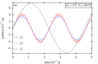
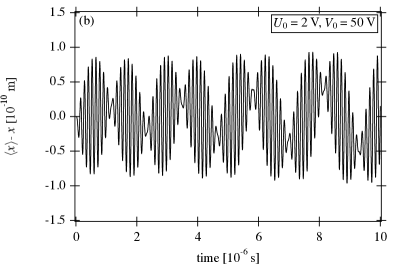
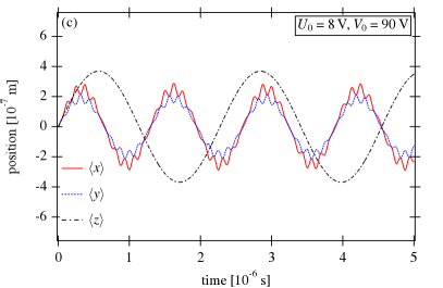
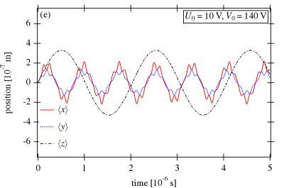
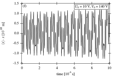
Figure 2: (Color online) Time evolution of the center-of-mass motion for different trap potentials: (a)–(b) $U_{0}=$2\text{\,}\mathrm{V}$$, $V_{0}=$50\text{\,}\mathrm{V}$$; (c)–(d) $U_{0}=$8\text{\,}\mathrm{V}$$, $V_{0}=$90\text{\,}\mathrm{V}$$; (e)–(f) $U_{0}=$10\text{\,}\mathrm{V}$$, $V_{0}=$140\text{\,}\mathrm{V}$$. Panels (a), (c), and (e) present the components of the expectation value of the center of mass, $\braket{\mathbf{r}}$ for the quantum trajectory. Panels (b), (d), and (f) present the difference between the quantum-mechanical expectation value $\braket{x}$ and the classical trajectory $x$.

For all three sets of parameters, we clearly see that $\braket{x}$ and $\braket{y}$ present an overall harmonic motion, on which micromotion is superposed, as expected (see Sec. 2.3). By contrast, the motion is harmonic in $z$, which is governed only by the ring-shaped electrodes, on which a static potential is applied. The frequency of the secular, harmonic motion also follows the dependence on $U_{0}$ and $V_{0}$ obtained form the classical model, Eqs. (14). A direct comparison between the quantum and classical trajectories is presented in Fig. 2(b), (d), and (f), for the $x$ component of the center-of-mass motion. We note that the absolute error is smaller than the grid spacing of the quantum simulation, $\Delta x=${10}^{-9}\text{\,}\mathrm{m}$$, but most importantly, it does not significantly grow with time, indicating that the periodicity of the motion is indeed the same.

4.2 Width of the wave packet

4.2.1 Spreading of the wave packet

One information that is not available from the classical simulation is the width of the wave packet and its possible growth. We have thus calculated, from the quantum simulations, the width of the wave packet, according to

$$\sigma_{\xi}\equiv\sqrt{\braket{\xi^{2}}-\braket{\xi}^{2}},$$ (38)

with $\xi\in\{x,y,z\}$. A sample result, for $\left(U_{0},V_{0}\right)=($10\text{\,}\mathrm{V}$,$140\text{\,}\mathrm{V}$)$, is shown in Fig. 3.

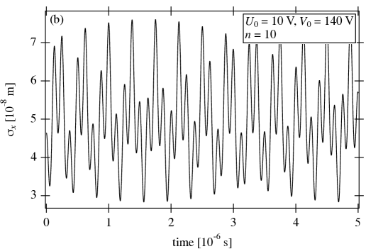
Figure 3: Width $\sigma_{x}$ of the wave packet, Eq. (38), for $U_{0}=$10\text{\,}\mathrm{V}$$, $V_{0}=$140\text{\,}\mathrm{V}$$, starting from the initial state: (a) Gaussian ground state of the effective potential [$n=0$ in Eq. (28)]; (b) excited state of the effective potential [$n=10$ in Eq. (28)].

We see that the width of the wave packet oscillates with time, but with that oscillation bounded, such that the ion remains completely inside the trap. This behavior is expected as the initial state chosen, see Sec. 3.1, corresponds to a Gaussian coherent state, which were previously shown to result in periodic oscillations of the width of the Gaussian.[23]

We have also done simulations for cases where the ion is not initially in the ground state of the effective potential [$n\neq 0$ in Eq. (27)], and thus obviously not a coherent state.[40] We find that such a situation leads to exactly the same motion of the center of mass. What is more striking is that the oscillation of the wave packet also presents the same behavior in both cases, see Fig. 3. Except for the amplitude of the oscillation, we see that the two cases follow the same temporal variation. This is evidenced also by the autocorrelation function

$$A_{x}(t)=\left|\Braket{\psi_{x}(x,0)}{\psi_{x}(x,t)}\right|^{2},$$ (39)

which is plotted in Fig. 4 for both $n=0$ and $n=10$, which show a return to the initial state after $2.26\text{\times}{10}^{-5}\text{\,}\mathrm{s}$ (we have checked that this result is independent of the choice of $n$).

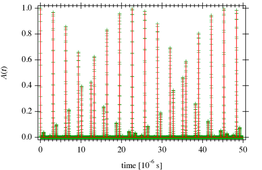
Figure 4: (Color online) Autocorrelation function for $U_{0}=$10\text{\,}\mathrm{V}$$, $V_{0}=$140\text{\,}\mathrm{V}$$, starting from: the initial state Gaussian ground state of the effective potential [$n=0$ in Eq. (28)] (crosses); the excited state of the effective potential [$n=10$ in Eq. (28)] (full line).

This recurrence, which depends on the parameters $U_{0}$ and $V_{0}$, corresponds to the time it takes for the classical trajectory to return to the same point in phase space, reinforcing the link between the classical and quantum trajectories, see Sec. 4.2.2. Due to the symmetry in the trapping field, see Eqs. (1)–(3), this recurrence time is also observed for $\psi_{y}(y,t)$. However, along the $z$ axis the ion has a simple harmonic motion, with a period of $2.03\text{\times}{10}^{-6}\text{\,}\mathrm{s}$, so the full autocorrelation function

$$A(t)=\left|\Braket{\psi(0)}{\psi(t)}\right|^{2},$$ (40)

doesn’t show any return to $A=1$.

4.2.2 Stability and spreading of the wave packet

Previous work has established that the motion of the center of mass of the wave packet should follow the same trajectory as that for a classical particle.[20, 21] As such, the stability criterion derived from the Mathieu equation, see Sec. 2.2, should apply also to the quantum dynamics,[19, 20] provided also that the oscillation of the width of the wave packet stays bounded, see Sec. 4.2.1.

We have checked this numerically by considering the border between stable and unstable trajectories, see Fig. 1. Using Mathematica,[41] we find that the Mathieu characteristic value $b_{1}$ for $U_{0}=$10\text{\,}\mathrm{V}$$ is at $V_{0}=$283.659\text{\,}\mathrm{V}$$. We ran simulations for points on either side of this border, choosing $V_{0}=$283.6\text{\,}\mathrm{V}$$ (stable) and $V_{0}=$283.66\text{\,}\mathrm{V}$$ (unstable), using now 1048576 grid points, in the range $[$-10\text{\,}\mathrm{\SIUnitSymbolMicro m}$,$10\text{\,}\mathrm{\SIUnitSymbolMicro m}$]$, to account for the wider oscillations of the wave packet. The results of the time evolution are presented in Fig. 5,

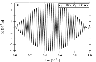
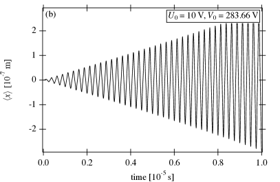
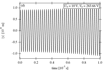
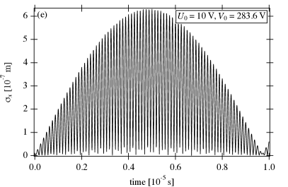
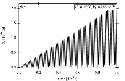
Figure 5: Time evolution of the center-of-mass motion and width of the wave packet: (a), (c), (e), and (g) $U_{0}=$10\text{\,}\mathrm{V}$$, $V_{0}=$283.6\text{\,}\mathrm{V}$$ (inside the stability region); (b), (d), (f), and (h) $U_{0}=$10\text{\,}\mathrm{V}$$, $V_{0}=$283.66\text{\,}\mathrm{V}$$ (outside the stability region).

with snapshots of the density distribution given in Fig. 6.

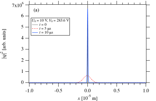
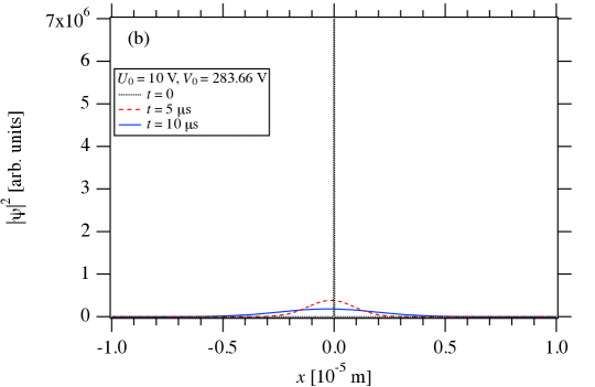
Figure 6: (Color online) Density distribution along the $x$ axis at times $t=0$, $5$, and $10\text{\,}\mathrm{\SIUnitSymbolMicro s}$ for: (a) the stable case $U_{0}=$10\text{\,}\mathrm{V}$$, $V_{0}=$283.6\text{\,}\mathrm{V}$$; (b) the unstable case $U_{0}=$10\text{\,}\mathrm{V}$$, $V_{0}=$283.66\text{\,}\mathrm{V}$$. Note that, in both cases, the wave packet at $t=0$ peaks at $\left|\psi_{x}(x=0)\right|^{2}\approx$5.7\text{\times}{10}^{7}$$, beyond the scale of the figures.

We find that the trajectory is indeed bounded for $V_{0}=$283.6\text{\,}\mathrm{V}$$, along all dimensions (results for the z-axis are not shown, as the motion is always simply harmonic along that direction). The width of the wave packet, Figs. 5(e) and (g), increases such that it extends farther than the center-of-mass trajectory, but still presents a bounded oscillatory behavior. In contrast, for $V_{0}=$283.66\text{\,}\mathrm{V}$$, the center-of-mass motion is an unbounded oscillation, and the ion will eventually escape the trapping region. Of particular interest is the fact that the width of the wave packet now also appears as an oscillation of increasing amplitude. This is particularly striking for the motion along the y-axis, where the trajectory diverges much more slowly than along the x-axis [due to the difference in the phase of the trapping field along those two directions, see Eq. (2)], the width of the wave packet grows with the same rate along both directions.

4.2.3 Floquet approximate solution

In Sec. 2.4, we presented the results of an approximate analytical solution, based on the Floquet theorem, from which we derived the a time-dependent width Eq. (22). We will now compare the result thus obtained with the equivalent quantum mechanical simulation. In other to satisfy the conditions of the approximate solution, namely $|a_{x}|,q_{x}^{2}\ll 1$, we take $U_{0}=$2\text{\,}\mathrm{V}$$, $V_{0}=$20\text{\,}\mathrm{V}$$, which corresponds to $a_{x}=-0.00151$, $q_{x}=-0.0645$. We see, Fig. 7,

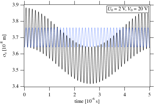
Figure 7: (Color online) Width $\sigma_{x}$ of the wave packet for $U_{0}=$2\text{\,}\mathrm{V}$$, $V_{0}=$20\text{\,}\mathrm{V}$$, for the approximate Floquet analytical solution Eq. (22) (dashed line), compared to the corresponding value from the numerical solution of the full time-dependent Schrödinger equation (solid line).

that the approximate solution reproduces well the oscillation at the trap frequency $\Omega$, but is off by a factor of $\sim 2$ in the amplitude of the oscillation of the width. It also doesn’t reproduce a longer-period oscillation that is present in the actual wave packet.

4.3 Validity of the effective potential approximation

For completeness, we also examine the the validity of effective potential approximation, by calculating the effective wave functions corresponding to $\psi_{\mathrm{eff}}$ [see Eq. (35)] for the same sets of $(U_{0},V_{0})$ as in Sec. 4.1 before and compared them with the actual time-dependent wave function by calculating the projection

$$P(t)=\left|\Braket{\psi_{x}(x,t)}{\psi_{\mathrm{eff},x}(x,t)}\right|^{2}.$$ (41)

Figure 8 presents results for $U_{0}=$2\text{\,}\mathrm{V}$,V_{0}=$50\text{\,}\mathrm{V}$$, which corresponds to $a\approx-1.5\times 10^{-3}$, $q\approx 0.45$; as mentioned in Sec. 3.2, this effective potential approximation is valid in the limit of small absolute values of $a$ and $q$.[3]

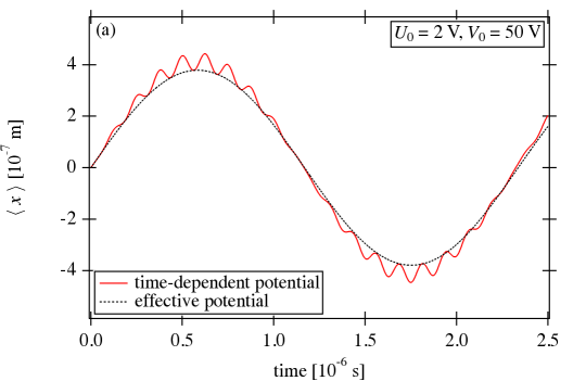
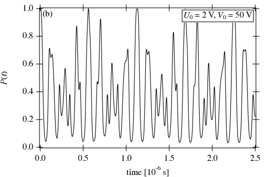
Figure 8: (Color online) (a) Time evolution of the center-of-mass motion calculated using the effective potential approximation vs. full quantum dynamics. (b) Projection of the phase-corrected effective wave function $\psi_{\mathrm{eff},x}$ on the exact wave function. The trapping field is $U_{0}=$2\text{\,}\mathrm{V}$,V_{0}=$50\text{\,}\mathrm{V}$$ ($a\approx-1.5\times 10^{-3}$, $q\approx 0.45$).

As expected, the effective potential solution reproduces the secular motion of the ion, see Fig. 8(a), but not the micromotion. The exact solution is recovered every quarter period of the oscillation, as the projection $P(t)$ shows [Fig. 8(b)], but in between the discrepancy between the exact and the effective solution can be almost complete. The non-corrected effective wave function $\phi_{\mathrm{eff}}$ is worse on average, although it does present more singular times where the projection $P(t)\approx 1$.

When increasing the trapping field to $U_{0}=$10\text{\,}\mathrm{V}$,V_{0}=$140\text{\,}\mathrm{V}$$, for which $a\approx-7.6\times 10^{-3}$ and $q\approx 0.16$, the effective potential approximation is no longer applicable, as can be seen in Fig. 9.

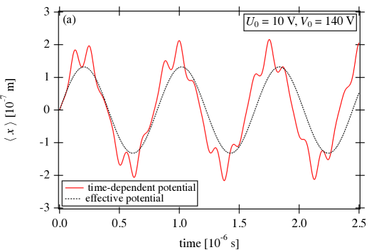
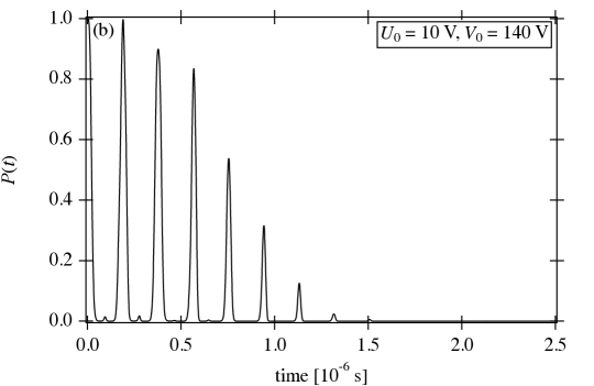
Figure 9: (Color online) (a) Time evolution of the center-of-mass motion calculated using the effective potential approximation vs. full quantum dynamics. (b) Projection of the phase-corrected effective wave function $\psi_{\mathrm{eff}}$ on the exact wave function. The trapping field is $U_{0}=$10\text{\,}\mathrm{V}$,V_{0}=$140\text{\,}\mathrm{V}$$ ($a\approx-7.6\times 10^{-3}$, $q\approx 0.16$).

The amplitude of the micromotion is so important that the trajectories appear to different oscillation periods (a similar effect can be seen in the width of the packet[19]). After a short time, $\psi_{\mathrm{eff}}$ differs completely from the exact wave function, as seen in Fig. 9(b), although a revival in $P(t)$ is expected when the secular motion and the micromotion resynchronize.

5 Conclusion

We have performed quantum simulations of the full dynamics of an ion in a linear Paul trap, including the time-dependent variation of the trapping potential. We have shown that the center-of-mass motion of the ion is well reproduced by the classical equations of motion, even outside the so-called stability region, where the trajectories are no longer bounded.[3] The use of the effective potential approximation[3, 15] allows one to get the average (secular) motion of the center of mass correct, but completely neglects the micromotion, which can be on par with the secular motion for certain trapping parameters, to a point where the results are completely different from the exact dynamics (Fig. 9).

Considering the oscillations of the width wave packet, we have found that they are bounded for stable trajectories, even when the wave packet is not Gaussian. This extends previous work that had demonstrated oscillations only for coherent wave packets,[19, 24, 22, 23] and will merit further investigation. The wave packet was also seen to continuously increase in width for conditions outside the stability region, while it remained bounded for stable trajectories. Our results confirm the Floquet analysis of the quantum dynamics that shows that the center of mass of the wave packet should follow the classical trajectory,[20, 21] and that the stability criterion based on classical trajectories also applies to quantum motion.[19, 20]

This study opens up the possibility of using semi-classical models for the simulation of trapped ions. The center-of-mass motion could be considered to be classical, while internal degrees of freedom could be treated quantum mechanically. This could greatly simplify, for instance, an extensive treatment of the interaction of a trapped atomic ion with laser pulses, or simulations of the trapping of molecular ions.

References

- [1] W. Paul, Rev. Mod. Phys. 62, 531 (1990).
- [2] P. K. Ghosh, Ion Traps (Oxford University Press, Oxford, 1995).
- [3] F. G. Major, V. N. Gheorghe, and G. Werth, Charged Particle Traps: Physics and Techniques of Charged Particle Field Confinement (Springer, Berlin, 2005).
- [4] M. Raizen, J. Gilligan, J. Bergquist, W. Itano, and D. Wineland, J. Mod. Opt. 39, 233 (1992).
- [5] M. G. Raizen, J. M. Gilligan, J. C. Bergquist, W. M. Itano, and D. J. Wineland, Phys. Rev. A 45, 6493 (1992).
- [6] B. Brkić, S. Taylor, J. F. Ralph, and N. France, Phys. Rev. A 73, 012326 (2006).
- [7] P. H. Dawson and N. R. Whetten, J. Vac. Sci. Technol. 5, 1 (1968).
- [8] M. D. N. Lunney, J. P. Webb, and R. B. Moore, J. Appl. Phys. 65, 2883 (1989).
- [9] F. A. Londry, R. L. Alfred, and R. E. March, J. Am. Soc. Mass. Spectrom. 4, 687 (1993).
- [10] H.-P. Reiser, R. K. Julian Jr., and R. G. Cooks, Int. J. Mass Spectrom. Ion Processes 121, 49 (1992).
- [11] G. Wu, R. G. Cooks, Z. Ouyang, M. Yu, W. J. Chappell, and W. R. Plass, J. Am. Soc. Mass. Spectrom. 17, 1216 (2006).
- [12] X.-G. Wu, Int. J. Mass Spectrom. 263, 59 (2007).
- [13] M. S. Herbane, Int. J. Mass Spectrom. 303, 73 (2011).
- [14] M. Cetina, A. T. Grier, and V. Vuletić, Phys. Rev. Lett. 109, 253201 (2012).
- [15] R. J. Cook, D. G. Shankland, and A. L. Wells, Phys. Rev. A 31, 564 (1985).
- [16] S. A. Gardiner, J. I. Cirac, and P. Zoller, Phys. Rev. A 55, 1683 (1997).
- [17] S.-B. Zheng, Phys. Lett. A 248, 25 (1998).
- [18] H. Moya-Cessa, F. Soto-Eguibar, J. M. Vargas-Martínez, R. Juárez-Amaro, and A. Zúñiga-Segundo, Phys. Rep. 513, 229 (2012).
- [19] F.-l. Li, Phys. Rev. A 47, 4975 (1993).
- [20] M. Combescure, Ann. Inst. Henri Poincaré, A 44, 293 (1986).
- [21] L. S. Brown, Phys. Rev. Lett. 66, 527 (1991).
- [22] R. J. Glauber, in Laser Manipulation of Atoms and Ions, edited by E. Arimondo, W. D. Phillips, and F. Strumia (North-Holland, Amsterdam, 1992), pp. 643–660.
- [23] R. J. Glauber, in Quantum Measurements in Optics, Vol. 282 of NATO ASI Series B: Physics, edited by P. Tombesi and D. F. Walls (Plenum Press, New York, 1992), pp. 3–14.
- [24] D. Leibfried, R. Blatt, C. Monroe, and D. Wineland, Rev. Mod. Phys. 75, 281 (2003).
- [25] K. Wang, M. Feng, and J. Wu, Phys. Rev. A 52, 1419 (1995).
- [26] D. J. Berkeland, J. D. Miller, J. C. Bergquist, W. M. Itano, and D. J. Wineland, J. Appl. Phys. 83, 5025 (1998).
- [27] D. J. Berkeland, J. D. Miller, J. C. Bergquist, W. M. Itano, and D. J. Wineland, Phys. Rev. Lett. 80, 2089 (1998).
- [28] H. Rohde, S. T. Gulde, C. F. Roos, P. A. Barton, D. Leibfried, J. Eschner, F. Schmidt-Kaler, and R. Blatt, J. Opt. B: Quantum Semiclass. Opt. 3, S34 (2001).
- [29] M. Drewsen and A. Brøner, Phys. Rev. A 62, 045401 (2000).
- [30] G. Wolf, in NIST Handbook of Mathematical Functions, edited by F. W. J. Oliver, D. W. Lozier, R. F. Boisvert, and C. W. Clark (Cambridge University Press, Cambridge, 2010), Chap. 28, pp. 651–681.
- [31] J. H. Shirley, Phys. Rev. 138, B979 (1965).
- [32] C. M. Dion, A. Hashemloo, and G. Rahali, Comput. Phys. Commun. 185, 407 (2014).
- [33] C. Cohen-Tannoudji, B. Diu, and F. Laloë, Quantum Mechanics (Wiley, New York, 1992).
- [34] P. Pechukas and J. C. Light, J. Chem. Phys. 44, 3897 (1966).
- [35] M. D. Feit, J. A. Fleck, Jr., and A. Steiger, J. Comput. Phys. 47, 412 (1982).
- [36] M. D. Feit and J. A. Fleck, Jr., J. Chem. Phys. 78, 301 (1983).
- [37] B. H. Bransden and C. J. Joachain, Physics of Atoms and Molecules, 2 ed. (Prentice Hall, Harlow, 2003).
- [38] E. Hairer, C. Lubich, and G. Wanner, Geometric Numerical Integration: Structure-Preserving Algorithms for Ordinary Differential Equations, 2 ed. (Springer, Berlin, 2006).
- [39] S. Urabe, M. Watanabe, H. Imajo, K. Hayasaka, U. Tanaka, and R. Ohmukai, Appl. Phys. B 67, 223 (1998).
- [40] J. R. Klauder and B.-S. Skagerstam, Coherent States: Applications in Physics and Mathematical Physics (World Scientific, Singapore, 1985).
- [41] Wolfram Research, Inc., Mathematica, Version 10.0 ed. (Wolfram Research, Inc., Champaign, Il., 2014).