On particle oscillations

Abstract

It has been firmly established, that neutrinos change their flavour during propagation. This feature is attributed to the fact, that each flavour eigenstate is a superposition of three mass eigenstates, which propagate with different frequencies. This picture, although widely accepted, is wrong in the simplest approach and requires quite sophisticated treatment based on the wave-packet description within quantum field theory. In this communication we present a novel, much simpler explanation and show, that oscillations among massive particles can be obtained in a natural way. We use the framework of quantum mechanics with time being a physical observable, not just a parameter.

1 Introduction

All elementary particles are subject to mixing within their respective groups, i.e., quarks, neutral leptons (neutrinos), charged leptons, as well as gauge bosons. This peculiar feature of gauge theories underlying the Standard Model comes from the requirement that the quantum numbers should match those observed in nature. In other words, in order to arrive at a picture consistent with the experiment, one has to ‘rotate’ sectors of the Standard Model, with the rotation parameters fitted from the experimental data. As a consequence of mixing, particles should oscillate between their possible states, as it is observed for neutrinos and some mesons.

However, from the theoretical point of view, not everything is clear in this picture. Take neutrino oscillations as an example. The widely accepted explanation is based on the assumption, that neutrinos which are paired with the charged leptons ($e$, $\mu$, $\tau$) are not the same as the propagating neutrinos. From the so-called interaction basis the interaction eigenstates $\nu_{\alpha}$, $\alpha=e,\mu,\tau$ have to be rotated by a unitary matrix to the physical basis, in which the states $\nu_{i}$, $i=1,2,3$ are those which propagate. The latter are physical particles with well defined masses, while the former are ill-defined, therefore virtual particles.

The immediate question which arises is, why do we have to work in two bases – one to describe interactions (with unrealistic particles with no definite mass) and another to describe propagation (of physical particles which are not observed in nature as standalone objects)? This counter-intuitive picture poses even more trouble when one wants to formulate a consistent description of, say, neutrino oscillations. Even assuming that in the process of emission three different physical particles are produced, each with well defined mass, momentum, and energy, it is difficult to justify, how these particles can arrive at the detection point as a single, detectable object. To resolve this problem different authors have argued, that these particles should share a common momentum or a common energy. Curiously, both approaches lead to the same final expression for the phase of oscillations. The same expression can also be reached when assuming nothing but neutrinos being ultra-relativistic [1]. The most correct derivation of the neutrino oscillations phase involves a full wave-packet treatment within quantum field theory [2].

In this communication we propose a different mechanism which leads to particle oscillations. Without referring to two different classes of states and working with the physical particles only we show, that under certain assumptions transitions between mass eigenstates can be observed. Our framework is the quantum mechanics in which time is no longer a parameter but one of the space-time variables.

2 The model

Recent experimental progress in the field of quantum mechanics suggests, that the ordinary formulation is not enough to properly describe what is being observed. In the so-called delayed-choice experiments [3, 4, 5] the cause and consequence seem to be inverted in time, implying that either causality is violated or our understanding of quantum phenomena should be altered. Also the newest experiments involving entangled systems [6] led to the conclusion, that within the traditional framework of quantum mechanics and special relativity, superluminal communication between different parts of the system is observed unless we change some basic principles in the formalism. Only recently, an entangled system of two photons that never co-existed in time has been created [7]. Another example is the observation of interference fringes [8] which are in agreement with the hypothesis, that the wave functions interfere in time, not in spatial variables.

Motivated by this line of research, a new quantum theory seems desirable, and one of such models has been proposed in Ref. [9]. One of its main features is the inclusion of time as an observable, such that it is possible to consistently construct a time operator [10]. Consequently, no time evolution of the wave function, which is space as well as time dependent, is needed. Each measurement is represented by a projection of the wave function on the states of a properly constructed ‘detector’, according to the Dirac projection postulate. This model successfully described such phenomena as: arrival time [11], delayed choice in quantum mechanics [9] and interference in time [12, 13].

In this communication we outline the description of the oscillations of mass eigenstates, which ultimately can be used to describe neutrino oscillations.

3 Particle oscillations

Keeping in mind neutrinos as our primary example, we want to show, that after emitting a particle of certain mass, another particle of a close laying mass can be observed. This all can happen under the assumption, that these particles share most if not all other properties, i.e., spin, electric charge etc.

We divide the process of describing particle oscillations into three stages:

1. the emission (creation) of the particle denoted by $\tau_{1}$,

2. propagation of the particle; for the sake of simplicity we assume free propagation and denote this stage by $\tau_{2}$,

3. detection of the particle ($\tau_{3}$).

According to the general rules given above, one has to construct projection operators describing each stage, and project the initial wave function of the emitted particle subsequently using the appropriate operators. The final outcome will represent the probability density of detecting the particle. Denoting by $\psi$ the initial wave function, the density matrix after the first stage is given by

$$\rho_{1}(\tau_{1})=|\psi\rangle\langle\psi|.$$ (1)

At the second stage the state changes into $\rho_{2}$ given by

$$\rho_{2}(\tau_{2})=\frac{\mathsf{E}\kern-1.0pt\hbox to0.0pt{\hss$|$}(\tau_{2})\rho_{1}(\tau_{1})\mathsf{E}\kern-1.0pt\hbox to0.0pt{\hss$|$}(\tau_{2})}{\hbox{ Tr}[\mathsf{E}\kern-1.0pt\hbox to0.0pt{\hss$|$}(\tau_{2})\rho_{1}(\tau_{1})\mathsf{E}\kern-1.0pt\hbox to0.0pt{\hss$|$}(\tau_{2})]},$$ (2)

where Tr denotes the trace, which provides proper normalisation of the expression, $\mathsf{E}\kern-1.0pt\hbox to0.0pt{\hss$|$}(\tau_{2})$ is the projection operator which here describes the propagation, and $\rho(\tau_{1})$ is given by Eq. (1). The detection process introduces yet another operator $\mathsf{E}\kern-1.0pt\hbox to0.0pt{\hss$|$}(\tau_{3})$ which defines the detector and acts according to

$$\rho_{3}(\tau_{3})=\frac{\mathsf{E}\kern-1.0pt\hbox to0.0pt{\hss$|$}(\tau_{3})\rho_{2}(\tau_{2})\mathsf{E}\kern-1.0pt\hbox to0.0pt{\hss$|$}(\tau_{3})}{\hbox{ Tr}[\mathsf{E}\kern-1.0pt\hbox to0.0pt{\hss$|$}(\tau_{3})\rho_{2}(\tau_{2})\mathsf{E}\kern-1.0pt\hbox to0.0pt{\hss$|$}(\tau_{3})]}.$$ (3)

Now, the probability of the process $\tau_{1}\to\tau_{2}\to\tau_{3}$ is given by

$$\hbox{ Prob}(\tau_{1}\to\tau_{2}\to\tau_{3})=\hbox{ Tr}[\mathsf{E}\kern-1.0pt\hbox to0.0pt{\hss$|$}(\tau_{3})\mathsf{E}\kern-1.0pt\hbox to0.0pt{\hss$|$}(\tau_{2})\rho_{1}(\tau_{1})\mathsf{E}\kern-1.0pt\hbox to0.0pt{\hss$|$}(\tau_{2})\mathsf{E}\kern-1.0pt\hbox to0.0pt{\hss$|$}(\tau_{3})].$$ (4)

To be more specific, let us assume three members of a family of particles having very similar masses. In the case of neutrinos, the mass differences are of the order of 10 meV or less which indicates really close laying states. Assume further that one of these particles is being created in a reaction. In the usual approach one neglects the time this reaction takes. It implies further that the produced particle appears immediately in zero-time, with sharp defined mass. On the other hand, if one takes into account that the reaction time is non-zero and finite, this introduces a kind of uncertainty in time for the particle to be produced, which results in a broadening of its energy profile. Thus, the created particle is no longer sharply peaked in mass, but possesses also an uncertainty in this parameter. One may also justify the broadening of mass of a particle in a more formal way. Namely, in our model the mass operator does not commute with the time operator. Therefore a kind of uncertainty relation between mass and time can formally be given, which prevents sharply peaked mass distribution to appear in any finite time.

The broadened mass profile overlaps with the neighbouring mass states, effectively turning into a linear combination of states with different masses, with the ‘mixing parameters’ given by the values of the function describing the profile (see Fig. 1 for a graphical representation).

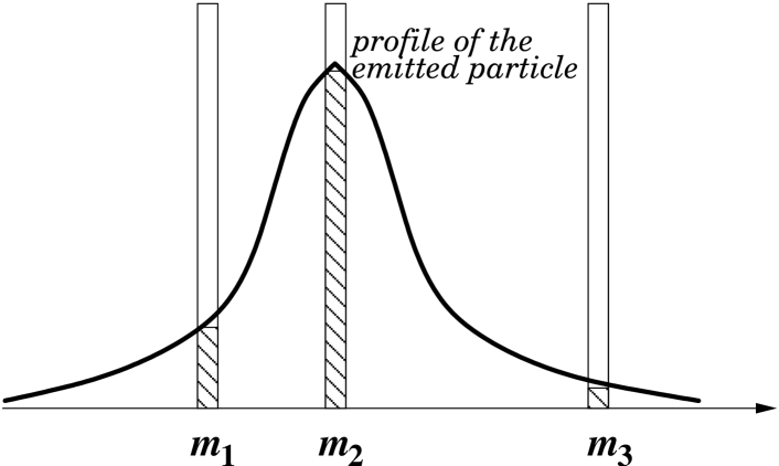
Figure 1: Schematic picture of the mass profile of the emitted particle. The emitted particle of central mass $m_{2}$ effectively has admixtures from masses $m_{1}$ and $m_{3}$.

Let us work, without loss of generality, in two dimensions, one time and one spatial variable $(t,x)$. It follows, that the wave function of the emitted particle may be written in the form

$$\psi(\tau_{1};t,x)=\int_{\mathbb{R}^{2}}d^{2}k\ a_{M}(k_{0},k_{1})\ \eta^{*}_{k}(t,x),$$ (5)

where $\tau_{1}$ denotes the first stage of the process, $\eta^{*}_{k}(t,x)=\eta^{*}_{k_{0}}(t)\ \eta^{*}_{k_{1}}(x)=\exp(-\mathrm{i}k_{0}t)\exp(-\mathrm{i}k_{1}x)/2\pi$, and the function $a_{M}(k_{0},k_{1})$ of the 2-momentum describes the shape of the particle in the momentum space. We notice for future reference, that $k_{0}^{2}-k_{1}^{2}=m^{2}$, so that it is possible to change the integration variables from $(k_{0},k_{1})$ to $(m^{2},k_{1})$.

The rules of the free propagation of the particle are governed by the structure of the vacuum. From this point of view the vacuum cannot distinguish the broadened state $\psi(\tau_{1})$ from three separate mass states propagating together. We therefore construct the projection operator describing the propagation as

$$\mathsf{E}\kern-1.0pt\hbox to0.0pt{\hss$|$}(\tau_{2})\psi(\tau_{1};t,x)=\int_{\Delta_{k}}d^{2}k\ \langle\eta_{k}^{*}(t,x)|\psi(\tau_{1};t,x)\rangle\eta_{k}^{*}(t,x),$$ (6)

where $\Delta_{k}$ is the set of 2-momenta, that can be transmitted through the vacuum during propagation. This, after a variable change $(k_{0},k_{1})\to(m^{2},k_{1})$, using the mass-shell relation, turns into a disjoint set of narrow peaks around $m_{1}$, $m_{2}$, and $m_{3}$. We therefore assume, that the structure of the vacuum permits propagation of some chosen set of masses, which defines our Standard Model. Evaluating Eq. (6) using (5) one gets

$$\mathsf{E}\kern-1.0pt\hbox to0.0pt{\hss$|$}(\tau_{2})\psi(\tau_{1};t,x)=\int_{\Delta_{k}}d^{2}k\ a_{M}(k_{0},k_{1})\eta_{k}^{*}(t,x).$$ (7)

Finally, let us denote the wave function of the detector by $\phi(\tau_{3};s,X)$. The detector is two-dimensional (one time and one spatial dimension) and located at the space-time point $(s,X)$. Notice, that by construction the measurement is time dependent. The projection operator representing the detection is now

$$\mathsf{E}\kern-1.0pt\hbox to0.0pt{\hss$|$}(\tau_{3})=|\phi(\tau_{3};s,X)\rangle\langle\phi(\tau_{3};s,X)|.$$ (8)

If we want to distinguish the detected particles by their masses, the detector function $\phi$ should describe states with definite mass, or should be peaked around some mass in the mass-momentum space. One such example is the infinite potential well described in the next section.

3.1 Example: infinite potential well

Let us represent the detector as eigenfunctions of the Klein–Gordon equation in a two-dimensional infinite potential well $\phi^{(s,X)}_{n_{0},n_{1}}(\tau_{3};t,x)$. Denote its dimensions and localisation by $L_{0}\times L_{1}$ with the central point $(s+L_{0}/2,X+L_{1}/2)$, i.e., it is a rectangle with the closer corner given by the space-time point $(s,X)$, extending by $L_{0}$ in the time direction and by $L_{1}$ in the spatial direction. The detector has to be tuned to detect certain mass $m_{D}$ given by

$$(m_{D})^{2}=\pi^{2}\left(\frac{n_{0}^{2}}{L_{0}^{2}}-\frac{n_{1}^{2}}{L_{1}^{2}}\right)$$ (9)

where $n_{0}$, $n_{1}$ sign different modes of the wave function within the well. The probability of detection is in this case given by

$$\hbox{ Prob}(\tau_{1}\to\tau_{3};s,X)=$$ (10)

$$\sum_{n_{0},n_{1}}\left|\int_{\Delta_{k}}d^{2}k\ \langle\eta_{k}^{*}|\psi(\tau_{1};x)\rangle\langle\phi^{(s,X)}_{n0,n_{1}}(\tau_{3};t,x)|\eta_{k}^{*}\rangle\right|^{2}.$$

Working out this example explicitly, the full formula reads

$$\hbox{ Prob}(\tau_{1}\to\tau_{3};s,X)=$$

$${\cal N}\sum_{n_{0},n_{1}}(n_{0}n_{1})^{2}\Bigg{|}\int_{\Delta_{(m^{2})}}d(m^{2})\int_{\mathbb{R}}dk\ \frac{a_{M}(m^{2},k)}{\sqrt{m^{2}+k^{2}}}$$

$$\times\exp\left\{-{\rm i}\left[\sqrt{m^{2}+k^{2}}L_{0}(s+1)+k(X+L_{1})\right]\right\}$$

$$\times\frac{\sin\left(\sqrt{m^{2}+k^{2}}\frac{L_{0}}{2}-n_{0}\frac{\pi}{2}\right)}{(m^{2}+k^{2})L_{0}^{2}-(n_{0}\pi)^{2}}\ \frac{\sin\left(k\frac{L_{1}}{2}-n_{1}\frac{\pi}{2}\right)}{(kL_{1})^{2}-(n_{1}\pi)^{2}}\Bigg{|}^{2},$$

where we have changed the variables to integrate over masses squared. Here $\cal N$ is an overall normalisation factor, and we recall that in normal units all masses should be read as $m/(\hbar c)$.

The region $\Delta_{(m^{2})}$ consists of three narrow peaks around the masses $m_{1}$, $m_{2}$, and $m_{3}$. One may therefore simplify the integral over $m^{2}$ and substitute it by a sum

$$\int_{\Delta_{(m^{2})}}d(m^{2})F(m^{2},k)\to\sum_{j=1,2,3}(4m_{j}\delta_{2})F(m_{j}^{2},k)$$

where $\delta_{2}$ is the (common, for simplicity) width of the peaks around the masses $m_{j}$, characteristic for the second stage $\tau_{2}$. This shows clearly that in the final formula (after the modulus squared is applied), interference terms involving different masses $m_{j}$ will appear, leading to possible oscillations. We have shown therefore, that the emission of one mass results in our model in a non-zero probability of detection of another mass. This probability is some function of the localisation of the detector in space-time. The detailed behaviour depends strongly on the construction of the initial wave function ($\psi(\tau_{1})$) and the detector ($\phi(\tau_{3})$). We will discuss a simpler numerical example in the next section.

4 The truncated cosine distribution

To better control which mass is emitted, let us write down the initial profile $a_{M}(k_{0},k_{1})$ as $a_{m_{0}^{2}}(m^{2},k_{1})$, with $m_{0}$ being the central value of the emitted mass. We propose in this example the following explicit form of the profile function:

$$a_{m_{0}^{2}}(m^{2},k_{1}) = \cos\left((m^{2}-m_{0}^{2})\frac{\pi}{\delta}\right)\hbox{ rect}_{\delta}(m^{2}-m_{0}^{2})$$ (12)

$$\times \hbox{ rect}_{W}(k_{1}),$$

which in the momentum space is given by

$$a_{m_{0}^{2}}(k_{0},k_{1}) = \cos\left((k_{0}^{2}-k_{1}^{2}-m_{0}^{2})\frac{\pi}{\delta}\right)$$

$$\times \hbox{ rect}_{\delta}(k_{0}^{2}-k_{1}^{2}-m_{0}^{2})\hbox{ rect}_{W}(k_{1}).$$

Here the box function $\hbox{ rect}_{w}(x)$ is a rectangle of width $w$, height 1, centred around 0 in the $x$ variable. The distribution (12) gives a cosine-shaped smearing of width $\delta$ in the masses squared around $m_{0}^{2}$, and a flat smearing in spatial momenta of width $W$. This choice is physically reasonable. The function $a_{m_{0}^{2}}(m^{2},k_{1})$ is depicted on Fig. 2 for some choice of the width parameters.

Figure 2: Plot of the profile function $a_{m_{0}^{2}}(m^{2},k)$ Eq. (12) for $m_{0}^{2}=5$, $\delta=2$, $W=2$.

We further assume, that the process of detection is in fact quite similar to the process of emission. In the case of neutrinos we expect them to be created and detected in a weak process, so the interaction vertexes in the Feynman diagrams are similar (e.g. a beta and an inverse-beta decay). Therefore we define both the initial wave function and the detector wave function in a similar way, i.e.,

$$\psi(t,x)=\int_{\mathbb{R}^{2}}d^{2}k\ a_{m_{0}^{2}}(k)\ \eta^{*}_{k}(t,x),$$ (14)

$$\phi(t,x)=\int_{\mathbb{R}^{2}}d^{2}k\ a_{m_{D}^{2}}(k)\ \eta^{*}_{k}(t,x),$$ (15)

$m_{0}$ and $m_{D}$ being the emitted and detected mass, respectively. Now, the detector needs to be shifted from the origin to the point $(s,X)$ resulting in

$$\phi(t,x)\to\phi(t-s,x-X)=e^{\mathrm{i}k_{0}s}e^{\mathrm{i}k_{1}X}\phi(t,x).$$ (16)

Finally, we arrive at the following formula for the probability of detection:

$$\hbox{ Prob}(s,X)={\cal N}\Bigg{|}\int_{\mathbb{R}}dk_{1}\int_{\Delta_{(m^{2})}}d(m^{2})$$

$$\frac{e^{\mathrm{i}\sqrt{m^{2}+k_{1}^{2}}s}e^{\mathrm{i}k_{1}X}}{\sqrt{m^{2}+k_{1}^{2}}}a_{m_{0}^{2}}(m^{2},k_{1})a_{m_{D}^{2}}(m^{2},k_{1})\Bigg{|}^{2},$$ (17)

where $\cal N$ is an overall normalisation factor and the functions $a$ are given by Eq. (12). The integration range $\Delta_{(m^{2})}$ consists of three narrow peaks around the masses $m_{1,2,3}$. Assuming the width of the peaks $\delta_{2}$ being small, one may approximate this integration by taking the value of the integrand in the central points times the width of the peaks, which yields

$$\hbox{ Prob}(s,X)={\cal N}\Bigg{|}\int_{\mathbb{R}}dk_{1}\sum_{j=1,2,3}(4m_{j}\delta_{2})$$

$$\frac{e^{\mathrm{i}\sqrt{m^{2}+k_{1}^{2}}s}e^{\mathrm{i}k_{1}X}}{\sqrt{m_{j}^{2}+k_{1}^{2}}}a_{m_{0}^{2}}(m_{j}^{2},k_{1})a_{m_{D}^{2}}(m_{j}^{2},k_{1})\Bigg{|}^{2}.$$ (18)

Notice that both $m_{0}$ and $m_{D}$ are one of the $m_{j}$’s.

First of all let us check the overall behaviour of the formula Eq. (4). We present a 3D plot of the values of Prob as a function of the localisation $(s,X)$ of the detector on Fig. 3. This is a neutrino-inspired example with the masses given by [14]

$$m_{1}=0.1\hbox{ eV},\quad m_{2}=m_{1}+\Delta m^{2}_{12},\quad m_{3}=m_{1}+\Delta m^{2}_{13}$$

$$\Delta m^{2}_{12}=7.6\times 10^{-5}\hbox{ eV}^{2},\qquad\Delta m^{2}_{13}=2.5\times 10^{-3}\hbox{ eV}^{2}.$$

The smearing parameters where chosen as

$$\delta_{0}=\delta_{D}=1.1\times\Delta m^{2}_{13},\qquad\delta_{2}=0.001\times\Delta m^{2}_{12}.$$

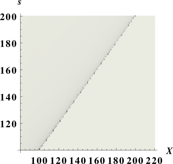
Figure 3: Density plot of the probability $\hbox{ Prob}(s,X)$ for $m_{0}=m_{3}$ and $m_{D}=m_{1}$. A clear maximum is visible for $s=X$.

Figure 4: Not normalised probabilities Eq. (4) of detection of $m_{1}$ (dashed lines) and $m_{3}$ (solid lines) if the mass $m_{0}=m_{1}$ (upper plot) and $m_{0}=m_{3}$ (lower plot) is emitted.

We first notice, that there is a strong maximum of the detecting probability along the $s=X$ line. This indicates, that the particles propagate with some maximum speed which corresponds approximately to the speed of light (in our units $c=1$). So the choice of small masses imply the particles being ultra-relativistic. Another feature is, that the probability is exactly zero until the fastest particles reach the point $s=X$ (lower light triangle), but remains non-zero for later times, as slower particles (or tails of the wave functions of particles that have already passed this point) may still be detected. This presents a physically consistent picture of particle propagation. Notice, that on Fig. 3 the case of $m_{0}\not=m_{D}$ is demonstrated.

A detailed analysis is shown on Fig. 4, on which we present the shapes of the detection probability functions for time $s=20$. We include the probabilities of detection of $m_{1}$ and $m_{3}$, when $m_{1}$ or $m_{3}$ is emitted. The curve describing $m_{2}$ will be lying in between these two. The probability is not normalised, so the units on the vertical axes are arbitrary. One clearly sees, that the probability shape is strongly peaked around $x=20$, which corresponds to the choice of $s$, and vanishes to zero for greater distances. Also, the maximum probability is obtained for the emitted mass, but some admixture of the other mass is also observed. This will lead to a drop in the observed flux of the particles, which is widely regarded as the proof of particle undergoing oscillations. In fact, with our choice of the profile function $a_{m^{2}}$ being proportional to the cosine, some oscillations of the probability of detection are also visible. These oscillations are better visible after the inclusion of proper normalisation ${\cal N}$, but we will discuss this topic in more detail in an upcoming paper.

5 Conclusions and outlook

We have shown, that particle oscillations may be a pure quantum mechanical phenomenon and do not require invoking unphysical interaction eigenstates. In our model the effect comes from the uncertainty principle after taking into account the fact, that no physical process can happen in zero-time. The broadening of mass spectrum of the emitted particle implies overlaps with the neighbouring mass states, which effectively adds them as admixtures to the propagating state. In this model it is natural, that heavier particles (like charged leptons for example) will not mix due to huge mass differences between them. The mixing of light quarks and almost no mixing between charged leptons is in excellent agreement with observations.

More work is needed to check, to which extent the effect depends on the detailed choice of the $a_{m^{2}}$ profile. We suspect, that each distribution (like Gaussian, inverted parabola etc.) should lead to similar results, but no formal proof of this statement has been constructed. It is also interesting to investigate this problem for different constructions of the detector.

The work of M.G. has been financed by the Polish National Science Centre under the decision number DEC-2011/01/B/ST2/05932.

References

- [1] Akhmedov E Kh and Smirnov A Yu 2009 Phys. Atom. Nucl. 72 1363
- [2] Beuthe M 2003 Phys. Rep. 375 105
- [3] Wheeler J A 1978 The ‘Past’ and the ‘Delayed-Choice Double-Slit Experiment’ Mathematical Foundations of Quantum Theory (Academic Press)
- [4] Grangier P, Roger G and Aspect A 1986 Europhys. Lett. 1 173
- [5] Jacques V et al. 2007 Science 315 966; Jacques V et al. 2006 arXiv:quant-ph/061024v1
- [6] Ma X-S et al. 2013 PNAS 110 1221
- [7] Megidish E et al. 2013 Phys. Rev. Lett. 110 210413
- [8] Lindner F et al. 2005 Phys. Rev. Lett. 95 040401
- [9] Góźdź A and Stefańska K 2008 J. Phys.: Conf. Ser. 104 012007
- [10] Góźdź A and Dȩbicki M 2007 Physics of Atomic Nuclei 70 529
- [11] Dȩbicki M and Góźdź A 2006 Int. J. Mod. Phys. E 15 437
- [12] Góźdź A, Dȩbicki M and Stefa ska K 2008 Physics of Atomic Nuclei 71 1
- [13] Dȩbicki M, Góźdź A and Stefańska K 2007 Int. J. Mod. Phys. E 16 616
- [14] Beringer J et al. (PDG) 2012 Phys. Rev. D 86 010001