Analysis of geometric phase effects in the quantum-classical Liouville formalism

Abstract

We analyze two approaches to the quantum-classical Liouville (QCL) formalism that differ in the order of two operations: Wigner transformation and projection onto adiabatic electronic states. The analysis is carried out on a two-dimensional linear vibronic model where geometric phase (GP) effects arising from a conical intersection profoundly affect nuclear dynamics. We find that the Wigner-then-Adiabatic (WA) QCL approach captures GP effects, whereas the Adiabatic-then-Wigner (AW) QCL approach does not. Moreover, the Wigner transform in AW-QCL leads to an ill-defined Fourier transform of double-valued functions. The double-valued character of these functions stems from the nontrivial GP of adiabatic electronic states in the presence of a conical intersection. In contrast, WA-QCL avoids this issue by starting with the Wigner transform of single-valued quantities of the full problem. Since the WA-QCL approach uses solely the adiabatic potentials and non-adiabatic derivative couplings as an input, our results indicate that WA-QCL can capture GP effects in general two-state crossing problems using first-principles electronic structure calculations without prior diabatization or introduction of explicit phase factors.

I Introduction

Molecular electronic adiabatic surfaces often cross forming degenerate manifolds of nuclear configurations with the topology of conical intersections (CIs).Migani and Olivucci (2004); Yarkony (1996) CIs are the most common triggers of radiationless transitions that drive photo-induced chemistry,Migani and Olivucci (2004) and transfers of electronic energy and charge. Blancafort, Hunt, and Robb (2005); Blancafort et al. (2001); Izmaylov et al. (2011) Besides facilitating electronic transitions CIs change the topology of the nuclear subspace: if adiabatic electronic wave functions are infinitely slowly (adiabatically) transported around a closed loop that encircles the CI seam, they acquire an extra $(-1)$ phase. This is the geometric phase (GP) that makes the electronic wave functions double-valued functions of nuclear coordinates.Longuet-Higgins et al. (1958); Berry (1984); Simon (1983); Ham (1987); Berry (1987); Aitchison (1988) In order to have a single-valued total electron-nuclear wave function, the nuclear wave functions have to compensate for sign changes in their electronic counterparts; hence, a nuclear Schrödinger equation must be solved with double-valued boundary conditions. The extra phase causes interference between parts of the nuclear wave function, which results in different vibronic spectra and nuclear dynamics as compared to the case without explicit account for the GP. Longuet-Higgins et al. (1958); Schön and Köppel (1994, 1995); Ryabinkin and Izmaylov (2013); Joubert-Doriol, Ryabinkin, and Izmaylov (2013)

The double-valued character of the nuclear wave functions in the adiabatic representation is challenging for numerical simulations. Switching to the diabatic representationCederbaum (2004) makes the nuclear diabatic wave function single-valued. However, the diabatic representation within a finite electronic subspace cannot be obtained Baer (1975) for a general polyatomic system ($N_{\text{atoms}}>2$), so one has to resort to approximate diabatization schemes. Köppel and Schubert (2006); Van Voorhis et al. (2010); Sirjoosingh and Hammes-Schiffer (2011); Yarkony (2012); Subotnik et al. (2009); Opalka and Domcke (2010); Troisi and Orlandi (2003); Papas, Schuurman, and Yarkony (2008); Nakamura and Truhlar (2001) To remain in the unambiguous adiabatic representation, Mead and Truhlar (1979) proposed to compensate for the GP of individual nuclear states by attaching an extra phase factor $e^{i\lambda(\mathbf{R})}$, where $\lambda(\mathbf{R})$ is a function that increases by $\pi$ on encircling a closed path around the CI seam. This approach was successfully implemented Kendrick and Mead (1995); Kendrick, Alden Mead, and Truhlar (2002); Kendrick (2003a) and applied to many real molecules by Kendrick.Kendrick and Pack (1996a, b); Kendrick (1997, 2003b) However, the definition of $\lambda(\mathbf{R})$ is based on diabatic model considerations, and its application to a general molecular system assumes some diabatic model potential. An alternative approach to the definition of $\lambda(\mathbf{R})$ was suggested by Baer and coworkers. Baer (1997); Xu, Baer, and Varandas (2000) They related $\nabla\lambda(\mathbf{R})$ to the matrix elements of derivative couplings $\mathbf{d}_{12}^{(1)}(\mathbf{R})$, thus removing any arbitrariness in the definition of $\lambda(\mathbf{R})$. However, this suggestion was challenged by Kendrick, Mead, and Truhlar (1999) who found that Baer’s approach inconsistently neglects some terms, and this inconsistency leads one to question the validity of the final result. Therefore, accounting for GP effects for general systems using only results of electronic structure calculations seems to be challenging within a fully quantum approach.

In this context, it is interesting that the quantum-classical Liouville (QCL) formalism Kapral (2006) is able to capture GP effects Kelly and Kapral (2010) using only adiabatic input: energies and non-adiabatic couplings. The QCL framework uses the Wigner transform (WT) of the nuclear degrees of freedom (DOF) to arrive at a mixed quantum-classical description. Derivations of the QCL equations for non-adiabatic problems using the adiabatic representation for electronic DOF can proceed along two paths that differ in the order in which the WT and the projection to the adiabatic basis are applied. We will denote by WA-QCL the approach where the WT is done first,Kapral and Ciccotti (1999) and by AW-QCL the approach where the adiabatic projection precedes the WT.Horenko et al. (2002); Ando and Santer (2003) It is not a priori obvious which of the two approaches is better. Previously, the WA-QCL and AW-QCL approaches were used to simulate the spin-boson model and no significant differences were found.Ando and Santer (2003) In this work we analyze the efficacy of these approaches to describe the dynamics in a two-dimensional (2D) linear vibronic coupling (LVC) model. As has been shown recently Ryabinkin and Izmaylov (2013), the 2D LVC model exhibits prominent GP effects, such as a distinct interference pattern due to the GP as well as a strong impact of the GP on nuclear dynamics. This model allows us to assess both QCL approaches with respect to CI-introduced topological features in non-adiabatic dynamics.

The paper is organized as follows: first, we briefly illustrate the emergence of double-valued adiabatic electronic wave functions in the 2D LVC model. Then, we outline the derivations of the matrix form of the WA-QCL equation starting from the full electron-nuclear density matrix Kapral and Ciccotti (1999) and the AW-QCL equation starting from a projection of the Liouville equation onto an adiabatic electronic basis. Horenko et al. (2002); Ando and Santer (2003) Comparing these two approaches we identify a term which is responsible for GP effects. We conclude our paper with numerical results and their analysis.

II Geometric phase in a two-dimensional linear vibronic coupling model

The two-dimensional LVC is a prototype for systems containing a CI and exhibiting nontrivial GP effects. The electron-nuclear Hamiltonian of the model is

$$\hat{\mathbf{H}}={\hat{T}}_{N}\mathbf{1}_{2}+\begin{pmatrix}\hat{V}_{11}&\hat{V}_{12}\\ \hat{V}_{12}&\hat{V}_{22}\end{pmatrix},$$ (1)

where ${\hat{T}}_{N}=-\frac{\hbar^{2}}{2}(\partial^{2}/\partial x^{2}+\partial^{2}/\partial y^{2})$ is the nuclear kinetic energy operator, $\hat{V}_{11}$ and $\hat{V}_{22}$ are the diabatic potentials represented by identical 2D parabolas shifted in the $x$-direction by $a$ and coupled by the $\hat{V}_{12}$ potential:

$${\hat{V}}_{11}={} \dfrac{\omega^{2}}{2}\left[\left(x+\dfrac{a}{2}\right)^{2}+y^{2}\right],\quad{\hat{V}}_{12}=cy,$$ (2)

$${\hat{V}}_{22}={} \dfrac{\omega^{2}}{2}\left[\left(x-\dfrac{a}{2}\right)^{2}+y^{2}\right].$$ (3)

Electronic DOF are represented as position-independent diabatic states $\ket{1}$ and $\ket{2}$ in a two-dimensional electronic subspace.

Transformation to the adiabatic representation is made by diagonalizing the potential matrix in Eq. (1) by means of the unitary transformation $U$

$$\mathbf{U}(\theta)=\begin{pmatrix}\cos\frac{\theta}{2}&-\sin\frac{\theta}{2}\\[4.30554pt] \sin\frac{\theta}{2}&\cos\frac{\theta}{2}\end{pmatrix},$$ (4)

where $\theta$ is a mixing angle between the diabatic states, and the factor $\frac{1}{2}$ is introduced for convenience. The adiabatic electronic wave functions are related to the columns of $U$ as

$$\ket{\psi_{1}^{\text{adi}}}={} \cos\frac{\theta}{2}\ket{1}+\sin\frac{\theta}{2}\ket{2}$$ (5)

$$\ket{\psi_{2}^{\text{adi}}}={} -\sin\frac{\theta}{2}\ket{1}+\cos\frac{\theta}{2}\ket{2}.$$ (6)

The angle $\theta$ is determined by the matrix elements of the diabatic Hamiltonian (1) as

$$\theta=\arctan\dfrac{2\,V_{12}}{V_{11}-V_{22}},$$ (7)

and changes by $2\pi$ for any closed path in the nuclear $(x,y)$ subspace that encircles the CI point. Considering that $U(2\pi)=-\mathbf{1}_{2}$, both adiabatic wave functions $\ket{\psi_{i}^{\text{adi}}}$ acquire an extra $(-)$ sign, which is a consequence of the GP. To have a single-valued total wave function

$$\ket{\Psi}=\ket{\chi_{1}^{\text{adi}}}\ket{\psi_{1}^{\text{adi}}}+\ket{\chi_{2}^{\text{adi}}}\ket{\psi_{2}^{\text{adi}}},$$ (8)

a sign change must be also imposed on the adiabatic nuclear wave functions $\ket{\chi_{1,2}^{\text{adi}}}$.

This consideration can be extended to the total density operator $\hat{\rho}=\ket{\Psi}\bra{\Psi}$, which is also a single-valued function of the nuclear $(x,y)$ coordinates. In contrast, the nuclear density matrix in the adiabatic representation

$$\hat{X}_{\alpha\alpha^{\prime}}=\Braket{\psi_{\alpha}^{\text{adi}}}{{\hat{\rho}}}{\psi_{\alpha^{\prime}}^{\text{adi}}}=\ket{\chi_{\alpha}^{\text{adi}}}\bra{\chi_{\alpha^{\prime}}^{\text{adi}}},$$ (9)

is a complicated object due to the double-value boundary conditions imposed on $\ket{\chi_{\alpha}^{\text{adi}}}$ and $\bra{\chi_{\alpha^{\prime}}^{\text{adi}}}$.

To model dynamics of the nuclear adiabatic densities $\hat{\mathbf{X}}$ we solve the corresponding Liouville equation

$$i\hbar\frac{\partial\hat{\mathbf{X}}}{\partial t}=[\hat{\mathbf{H}}^{\text{adi}},\hat{\mathbf{X}}].$$ (10)

Here, the Hamiltonian $\hat{\mathbf{H}}^{\text{adi}}$ is obtained by projecting the electronic DOF in Hamiltonian (1) onto the $\ket{\psi_{1,2}^{\text{adi}}}$ subspace:

$$\hat{\mathbf{H}}^{\text{adi}}=\begin{pmatrix}\hat{T}_{N}+\hat{\bm{\tau}}_{11}+{\hat{W}}_{-}&\hat{\bm{\tau}}_{12}\\ \hat{\bm{\tau}}_{21}&\hat{T}_{N}+\hat{\bm{\tau}}_{22}+{\hat{W}}_{+}\end{pmatrix},$$ (11)

where

$$\begin{split}\hat{\bm{\tau}}_{ij}={}&-\hbar^{2}[\langle\psi_{i}^{\text{adi}}|\nabla\psi_{j}^{\text{adi}}\rangle\cdot\nabla+\frac{1}{2}\langle\psi_{i}^{\text{adi}}|\nabla^{2}\psi_{j}^{\text{adi}}\rangle]\\ {}\equiv{}&-\hbar^{2}[\mathbf{d}_{ij}^{(1)}\cdot\nabla+\frac{1}{2}d_{ij}^{(2)}].\end{split}$$ (12)

with $\nabla=(\partial/\partial x,\partial/\partial y)$. The non-adiabatic couplings, $\mathbf{d}_{ij}^{(1)}$ and $d_{ij}^{(2)}$ are the vector and scalar derivative coupling matrix elements, and $\hat{W}_{\pm}$ are the matrix elements of the adiabatic potential $\mathbf{\hat{W}}=\mathbf{U\hat{V}U}^{\dagger}$:

$$\hat{W}_{\pm}=\frac{\hat{V}_{11}+\hat{V}_{22}}{2}\pm\frac{1}{2}\sqrt{(\hat{V}_{11}-\hat{V}_{22})^{2}+4\hat{V}_{12}^{2}}.$$ (13)

Equation (10) has to be solved by imposing double-value boundary conditions for $\hat{X}_{\alpha\alpha^{\prime}}$ due to the presence of the nontrivial GP. Single-valued boundary conditions lead to a completely different dynamics as shown in Fig. 1.

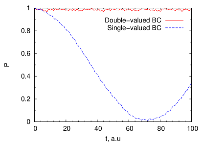
Figure 1: The solutions of Eq. (10) with double- and single-valued boundary conditions. The initial wavepacket is a simple Gaussian located in the left well; $P$ is the fraction of the wavepacket located in the left well. The model parameters are $\omega=2,a=3,c=4$.

To avoid GP complications in this model one can simulate dynamics for the diabatic nuclear density

$$\hat{\rho}_{\alpha\alpha^{\prime}}=\Braket{\alpha}{{\hat{\rho}}}{\alpha^{\prime}}=\ket{\chi_{\alpha}^{\text{dia}}}\bra{\chi_{\alpha^{\prime}}^{\text{dia}}},$$ (14)

by solving the corresponding Liouville equation

$$i\hbar\frac{\partial\hat{\bm{\rho}}}{\partial t}=[\hat{\mathbf{H}},\hat{\bm{\rho}}].$$ (15)

Of course, this diabatic path cannot be strictly followed for real molecules where the diabatic representation is not rigorously defined. But in this work we will use the diabatic representation to generate the exact quantum dynamics for our model problem.

III Quantum-classical Liouville formalism

In what follows we review the main steps of the WA-QCLKapral and Ciccotti (1999) and AW-QCL Horenko et al. (2002); Ando and Santer (2003) derivations to see the consequences of the double-valued character of the adiabatic electronic states in both approaches. We consider only a single set of nuclear coordinates associated with a particle of mass $M$ to simplify our discussion and to remain close to that in Sec. II; generalization to include additional nuclear coordinates is straightforward.

III.1 Wigner-then-adiabatic path

In line with Ref. Kapral and Ciccotti, 1999 we start with the WT of the nuclear DOF in the Liouville equation for the total density matrix in the coordinate representation $\hat{\rho}(\mathbf{r},\mathbf{R},\mathbf{r}^{\prime},\mathbf{R}^{\prime})=\Psi^{*}(\mathbf{r},\mathbf{R})\Psi(\mathbf{r}^{\prime},\mathbf{R}^{\prime})$,

$$i\hbar\frac{\partial\hat{\rho}_{W}}{\partial t}=(\hat{H}\hat{\rho})_{W}-(\hat{\rho}\hat{H})_{W}.$$ (16)

Here, we used the Wigner representation for operators

$$\hat{A}_{W}(\mathbf{R}_{c},\mathbf{P})=\int\left\langle\mathbf{R}_{c}+\frac{\mathbf{s}}{2}\right|\hat{A}\left|\mathbf{R}_{c}-\frac{\mathbf{s}}{2}\right\rangle e^{-\frac{i}{\hbar}\mathbf{s}\cdot\mathbf{P}}d\mathbf{s},$$ (17)

where $\mathbf{R}_{c}=(\mathbf{R}+\mathbf{R}^{\prime})/2$ is the position of the “coordinate centroid”, $\mathbf{s}=\mathbf{R}-\mathbf{R}^{\prime}$, and $\mathbf{P}$ is a parameter that can be associated with the classical momentum in the classical limit. Operator products $\left(\hat{A}\hat{B}\right)_{W}$ can be transformed further using the Wigner-Moyal operatorİmre et al. (1967) $e^{-i\hbar\hat{\Lambda}/2}$ as

$$\left(\hat{A}\hat{B}\right)_{W} = \hat{A}_{W}e^{-i\hbar\hat{\Lambda}/2}\hat{B}_{W},$$ (18)

where $\hat{\Lambda}$ is the Poisson bracket operator $\hat{\Lambda}=\overleftarrow{\nabla}_{\mathbf{P}}\cdot\overrightarrow{\nabla}_{\mathbf{R}_{c}}-\overleftarrow{\nabla}_{\mathbf{R}_{c}}\cdot\overrightarrow{\nabla}_{\mathbf{P}}$, and the arrows indicate the directions in which the differential operators act. Using identity (18) the Wigner-transformed Liouville equation becomes

$$i\hbar\frac{\partial\hat{\rho}_{W}}{\partial t}=\hat{H}_{W}e^{-i\hbar\hat{\Lambda}/2}\hat{\rho}_{W}-\hat{\rho}_{W}e^{-i\hbar\hat{\Lambda}/2}\hat{H}_{W}.$$ (19)

The $\hat{\Lambda}$ operator acts only on the nuclear DOF, thus, to introduce a semi-classical description of nuclear dynamics we expand the exponent in a Taylor series and keep only terms linear in $\hbar$:

$$i\hbar\frac{\partial\hat{\rho}_{W}}{\partial t} = \hat{H}_{W}\left(1-i\hbar\hat{\Lambda}/2\right)\hat{\rho}_{W}$$ (20)

$$-\hat{\rho}_{W}\left(1-i\hbar\hat{\Lambda}/2\right)\hat{H}_{W}.$$

The partially Wigner-transformed $H_{W}$ derived from Eq. (1) is quadratic in $\mathbf{R}$ and $\mathbf{P}$, hence, the Wigner-transformed Liouville equation (20) is exact for our model case.

Both the Wigner-transformed density matrix $\hat{\rho}_{W}$ and Hamiltonian $\hat{H}_{W}$ in Eq. (20) are still quantum operators in the electronic subspace. Let us project the electronic DOF on the adiabatic electronic eigenfuctions $\ket{\psi_{\alpha}^{\text{adi}}(\mathbf{R}_{c})}$

$$i\hbar\frac{\partial\hat{\rho}_{W}^{\alpha\alpha^{\prime}}}{\partial t}={} \bra{\psi_{\alpha}^{\text{adi}}}\hat{H}_{W}\left(1-\frac{i\hbar}{2}\hat{\Lambda}\right)\hat{\rho}_{W}\ket{\psi_{\alpha^{\prime}}^{\text{adi}}}$$

$${}-{} \bra{\psi_{\alpha}^{\text{adi}}}\hat{\rho}_{W}\left(1-\frac{i\hbar}{2}\hat{\Lambda}\right)\hat{H}_{W}\ket{\psi_{\alpha^{\prime}}^{\text{adi}}}.$$ (21)

Inserting the resolution-of-the-identity operator in the electronic subspace ${\hat{I}}=\sum_{\beta}\ket{\psi_{\beta}^{\text{adi}}(\mathbf{R}_{c})}\bra{\psi_{\beta}^{\text{adi}}(\mathbf{R}_{c})}$ between the operator products, we express Eq. (III.1) in terms of operator matrices defined as $\mathbf{A}_{W}\equiv\braket{\psi_{\alpha}^{\text{adi}}}{\hat{A}_{W}}{\psi_{\alpha^{\prime}}^{\text{adi}}}$

$$\frac{\partial{\bm{\rho}}_{W}}{\partial t} {}=-\frac{i}{\hbar}[\mathbf{H}_{W},{\bm{\rho}}_{W}]-\frac{1}{2}\left(\mathbf{H}_{W}\hat{\Lambda}{\bm{\rho}}_{W}-{\bm{\rho}}_{W}\hat{\Lambda}\mathbf{H}_{W}\right)$$

$$+\frac{1}{2}\Big{(}[\mathbf{D},\mathbf{H}_{W}]\cdot\nabla_{\mathbf{P}}{\bm{\rho}}_{W}+\nabla_{\mathbf{P}}{\bm{\rho}}_{W}\cdot[\mathbf{D},\mathbf{H}_{W}]\Big{)}$$

$$-\frac{\mathbf{P}}{M}\cdot[\mathbf{D},{\bm{\rho}}_{W}],$$ (22)

where $\mathbf{D}$ is the matrix of the vector derivative couplings $\mathbf{d}_{\alpha\beta}^{(1)}$. Equation (III.1) accounts for mutual interactions between the electronic and nuclear DOF. Note that all Wigner-transformed operators depend on a single nuclear coordinate $\mathbf{R}_{c}$, and even though the adiabatic functions $\ket{\psi_{\alpha}^{\text{adi}}(\mathbf{R}_{c})}$ are double-valued, the diagonal density matrix elements $\braket{\psi_{\alpha}^{\text{adi}}}{\hat{\rho}_{W}}{\psi_{\alpha}^{\text{adi}}}$ are all single-valued functions of $\mathbf{R}_{c}$. As for the off-diagonal elements $\braket{\psi_{\alpha}^{\text{adi}}}{\hat{\rho}_{W}}{\psi_{\beta}^{\text{adi}}}$ (coherences), in general, they are double-valued functions, because the GP related sign flip of the bra and ket components may not be simultaneous for any closed contour in the $\mathbf{R}_{c}$ subspace. An example of such situation is a three-state model where two electronic states $\ket{\psi_{1,2}^{\text{adi}}}$ have a CI, and the third state $\ket{\psi_{3}^{\text{adi}}}$ has an avoided crossing with the first two states. In this example, the matrix elements $\braket{\psi_{\alpha}^{\text{adi}}}{\hat{\rho}_{W}}{\psi_{3}^{\text{adi}}}_{\alpha=1,2}$ are double-valued functions because the sign change in $\bra{\psi_{1,2}^{\text{adi}}}$ is not compensated by that in $\ket{\psi_{3}^{\text{adi}}}$ on encircling the CI. Thus, generally, Eq. (III.1) must be simulated with double-valued boundary conditions for the off-diagonal elements. However, for problems where the parametric dependence of all adiabatic states leads to the same GP change after encircling any closed contour all matrix elements in Eq. (III.1) are single-valued functions, and Eq. (III.1) does not need double-valued boundary conditions. Our 2D LVC model is an example where the latter condition is satisfied because both functions $\ket{\psi_{1}^{\text{adi}}(\mathbf{R}_{c})}$ and $\ket{\psi_{2}^{\text{adi}}(\mathbf{R}_{c})}$ either change their sign or do not depending on whether the CI point is enclosed by the contour. At any case, all quantities in Eq. (III.1) are well defined mathematically, and their physical interpretation is well-known.Kapral and Ciccotti (1999)

III.2 Adiabatic-then-Wigner path

We start by projecting the Liouville equation onto the adiabatic electronic basis $\ket{\psi_{\alpha}^{\text{adi}}}$ to obtain

$$i\hbar\frac{\partial{\hat{X}}_{\alpha\alpha^{\prime}}}{\partial t}=\sum_{\beta}\left(\hat{H}^{\text{adi}}_{\alpha\beta}\,{\hat{X}}_{\beta\alpha^{\prime}}-{\hat{X}}_{\alpha\beta}\,\hat{H}^{\text{adi}}_{\beta\alpha^{\prime}}\right),$$ (23)

where ${\hat{H}}^{\text{adi}}_{\alpha\beta}$ and ${\hat{X}}_{\alpha\beta}$ are multi-state generalizations of the two-state adiabatic Hamiltonian (11) and nuclear density (9). Applying the WT to Eq. (23) we obtain

$$i\hbar\frac{\partial\mathbf{X}_{W}}{\partial t} {}=\mathbf{H}^{\text{adi}}_{W}e^{-i\hbar\hat{\Lambda}/2}\mathbf{X}_{W}-\mathbf{X}_{W}e^{-i\hbar\hat{\Lambda}/2}\mathbf{H}^{\text{adi}}_{W}.$$ (24)

For the double-valued adiabatic densities ${\hat{X}}_{\alpha\alpha^{\prime}}$ the WT

$$X_{W}^{\alpha\alpha^{\prime}}=\int\Braket{\mathbf{R}_{c}+\frac{\mathbf{s}}{2}}{\hat{X}_{\alpha\alpha^{\prime}}}{\mathbf{R}_{c}-\frac{\mathbf{s}}{2}}e^{-\frac{i}{\hbar}\mathbf{s}\cdot\mathbf{P}}d\mathbf{s}$$ (25)

is not well defined, because, as is shown in the Appendix, this operation is equivalent to the Fourier transform of a double-valued function. Unless special care is taken at this step the double-valued character of the ${\hat{X}}_{\alpha\alpha^{\prime}}$ density will be lost. Here, we follow previous derivationsHorenko et al. (2002); Ando and Santer (2003) of the AW-QCL equation, noting that it is inconsistent with subtleties arising from a nontrivial GP.

The Wigner-transformed adiabatic Hamiltonian $\mathbf{H}_{W}^{\text{adi}}$ in Eq. (24) differs from the $\mathbf{H}_{W}$ matrix only by the WT of the non-adiabatic coupling operators ${\hat{\bm{\tau}}}_{\alpha\beta}$ [see Eq. (12)],

$$\mathbf{H}^{\text{adi}}_{W}=\mathbf{H}_{W}+{\bm{\tau}}_{W},$$ (26)

where the ${\bm{\tau}}_{W}$ matrix has elements

$${\bm{\tau}}_{W}^{\alpha\alpha^{\prime}}=-i\hbar\frac{\mathbf{P}}{M}\cdot\mathbf{d}^{(1)}_{\alpha\alpha^{\prime}}+\frac{\hbar^{2}}{2M}\left(\nabla_{\mathbf{R}_{c}}\cdot\mathbf{d}^{(1)}_{\alpha\alpha^{\prime}}-d^{(2)}_{\alpha\alpha^{\prime}}\right).$$ (27)

The last term in the parentheses defines a positive-definite matrix $\mathbf{K}$ with elements

$$K_{\alpha\alpha^{\prime}}=\frac{\hbar^{2}}{2M}\left(\nabla\cdot\mathbf{d}^{(1)}_{\alpha\alpha^{\prime}}-d^{(2)}_{\alpha\alpha^{\prime}}\right)=\frac{\hbar^{2}}{2M}\braket{\nabla\psi_{\alpha}^{\text{adi}}}{\nabla\psi_{\alpha^{\prime}}^{\text{adi}}}.$$ (28)

The explicit form of the adiabatic Hamiltonian obtained from Eqs. (26–28) is

$$\mathbf{H}^{\text{adi}}_{W}=\mathbf{H}_{W}-i\hbar\frac{\mathbf{P}}{M}\cdot\mathbf{D}+\hbar^{2}\mathbf{K}.$$ (29)

Expanding the Wigner-Moyal exponent in the Taylor series and keeping only first order terms in $\hbar$ in Eq. (24) we obtain the AW-QCL equation,

$$\frac{\partial\mathbf{X}_{W}}{\partial t} {}=-\frac{i}{\hbar}\left[\mathbf{H}_{W},\mathbf{X}_{W}\right]-\frac{1}{2}\left(\mathbf{H}_{W}\hat{\Lambda}\mathbf{X}_{W}-\mathbf{X}_{W}\hat{\Lambda}\mathbf{H}_{W}\right)$$

$$-\frac{\mathbf{P}}{M}\cdot\left[\mathbf{D},\mathbf{X}_{W}\right].$$ (30)

It is important to note that Eq. (30) is no longer an exact evolution equation for the quantum dynamics of our 2D LVC model. This is in contrast to Eq. (20) which is fully equivalent to the quantum Liouville equation for this model. The difference stems from two sources: First, the adiabatic Hamiltonian [Eq. (29)] is not a quadratic function of the nuclear coordinates, and consequently the truncation of the Wigner–Moyal exponent is no longer exact. Second, the AW-QCL derivation ignores the double-valued character of the nuclear density, which results in Eq. (30) that corresponds to the evolution of a nuclear density with the incorrect (single-valued) boundary conditions. Comparing Eqs. (III.1) and (30) reveals that both sources of the difference between the AW-QCL and WA-QCL approaches can be related to the third term in Eq. (III.1). Since this term accounts for direct changes in the nuclear momenta as a result of coupling to the electronic DOF, one might expect significant influence of this term on the nuclear dynamics. Moreover, as we shall see below, neglecting this term leads to loss of GP related features in the nuclear dynamics.

IV Numerical simulations

To quantify the difference between the WA-QCL and AW-QCL approaches and to assess the relative importance of GP effects we simulate non-adiabatic dynamics for the 2D LVC model. Our choice of initial conditions and the model parameters aims to minimize differences between the WA-QCL and AW-QCL approaches that are related to the omission of the higher order quantum contributions in AW-QCL. We employ the following set of parameters for the 2D LVC model [Eqs. (1–3)]: $\omega=2$, $a=1$, $c=4$, $M=1$. The initial density is taken as a product of two Gaussian wave packets centred at the minimum of the $\ket{1}$ diabatic surface $(-a/2,0)$ with widths $\sigma=\sqrt{2/\omega}$ and an initial momentum $(5/2,0)$ (motion towards the positive $x$ values). This setup results in a relatively high initial energy and reduction of quantum tunnelling. We consider four different approaches to non-adiabatic dynamics: a) quantum diabatic [Eq. (15)], b) quantum adiabatic without GPEq. (10), c) WA-QCL, d) AW-QCL. We investigate two properties: the time evolution of the fraction of the nuclear density remaining in the region $x<0$ (Fig. 2), and the 2D nuclear adiabatic density at a given time (Fig. 3). The former is an integral property, which illustrates differences in dynamics, while the latter zooms into these differences at a given time.

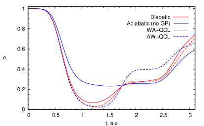
Figure 2: The fraction of the probability density remaining in the region $x<0$ ($P$) for the 2D LVC model simulated with different methods.

As expected, the WA-QCL dynamics is very close to that of the full quantum dynamics (see Fig. 2); the differences are due mainly to rather modest convergence of the WA-QCL density with respect to the number of classical trajectories in the employed Trotter-based simulation algorithmKernan, Ciccotti, and Kapral (2008) and use of the “momentum jump” approximationKapral and Ciccotti (1999) for the last two terms in Eq. (III.1). Both approaches predict almost full transfer of the density from the initial $x<0$ region to the $x>0$ region in a time of $1.3$ a.u. with some degree of recurrence at later times. By contrast, the quantum adiabatic dynamics exhibits less prominent population transfer. Results of AW-QCL differ from those of the other methods, which means that effects from the Wigner-Moyal exponent truncation are still comparable to GP effects. To elucidate the differences between the methods we present the two-dimensional nuclear density at $t=1.6$ a.u. (Fig. 3).

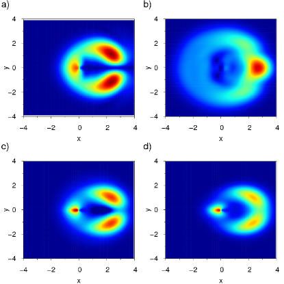
Figure 3: Snapshots of the square root of the probability density at t = 1.6 a.u. for the 2D LVC model dynamics: a) fully quantum (diabatic) , b) quantum adiabatic (no GP), c) WA-QCL, d) AW-QCL.

The fully quantum model with GPFig. 3(a) and the WA-QCL model [Fig. 3(c)] develop a nodal line in the region $x>0$. This prominent feature is completely absent in the quantum adiabatic dynamics [Fig. 3(b)] and, thus, can be seen as a manifestation of the GP. Schön and Köppel (1994); Ferretti et al. (1996); Kelly and Kapral (2010); Joubert-Doriol, Ryabinkin, and Izmaylov (2013) Moreover, the adiabatic model predicts completely spurious constructive interference between parts of the wave packet that skirt the CI point from opposite sides, giving rise to a peak in the nuclear density at $x\approx 2.5$ a.u. [see Fig. 3(b)]. The AW-QCL density is somewhat between those from both quantum models: it has a visible dip along the $y=0$ line, however, this dip is not as pronounced as for the models accounting for the GP. The AW-QCL density profile suggests that this approach does not produce any nuclear interference. To support this assertion we considered different relations between two spatially separated Gaussian wave packets.

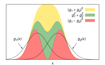
Figure 4: Total density of two Gaussian wave packets $g_{1}$ and $g_{2}$ in cases of (gold) constructive interference, (red) destructive interference, (green) no interference.

Figure 4 shows that in the absence of interference the total density may have a central minimum, which, however, is not as deep as in the case of destructive interference. This result also indicates that electronic transitions constitute the dominant quantum effect in the AW-QCL dynamics, while quantum nuclear interference within each electronic state is negligible.

V Conclusions

The analysis of the QCL dynamics for the 2D LVC model presented above showed that the WA-QCL equation is the only approach where complications arising from a non-trivial GP in the adiabatic representation do not make formalism ill-defined. In situations when the GP behavior of the electronic adiabatic states involved in the dynamics is similar (e.g., CI of two electronic states), the WA-QCL approach can treat GP effects exactly without imposing double-valued boundary conditions. In contrast, the AW-QCL approach involves the WT integral of the adiabatic density operator with a double-valued kernel. Practically, this transformation is equivalent to the Fourier transformation of a double-valued function, which is not a well-defined procedure. Yet, if one proceeds with the Fourier transformation ignoring the double-valued character of the quantum density, the resulting AW-QCL equation describes the quantum density with the incorrect single-valued boundary conditions. Thus, the AW-QCL approach is plagued by the same problems as the quantum dynamics in the adiabatic representation without including the GP (see Fig. 1).

Interestingly, the AW-QCL and WA-QCL equations differ only by one term. This term is responsible for differences associated with the Moyal–Wigner exponent truncation in different representations and GP effects. Further separation of the GP-related terms from those corresponding to the Moyal–Wigner exponent truncation does not seem to be feasible. However, this analysis suggests why the previous numerical assessmentAndo and Santer (2003) of the two approaches did not find a significant difference between results for the spin-boson model where GP effects are absent.

It is worth noting that in contrast to the quantum adiabatic picture, where the GP appears in the form of non-trivial boundary conditions, the WA-QCL approach confronts the problem of the GP in much milder fashion. The WT maps similar GP behavior of different electronic states into the third term of the WA-QCL dynamical equation (III.1). Thus, the only components that are left with the double-valued boundary conditions are coherences of electronic states that have different GP behaviors. An interesting question for future investigation is whether the trajectory based techniques used to simulate Eq. (III.1) will be able to handle the double-valued character of the coherences in general multi-level systems owing to the space locality of a propagated object?

It should be also emphasized that the WA-QCL approach, though accounting for the GP in our model, cannot be reduced to the Mead and Truhlar Mead and Truhlar (1979) treatment of the GP. This can be easily seen by considering a single electronic state version of Eq. (III.1) that describes classical dynamics of nuclear DOF on a given electronic potential without any GP terms, which inevitably appear in the Mead and Truhlar treatment.

All quantities that are required to perform WA-QCL dynamics, such as the adiabatic potentials and the derivative couplings, are readily available from first-principles quantum chemistry calculations. Thus, the WA-QCL formalism is probably the only formalism that can naturally account for GP effects in two electronic state crossing problems with on-the-fly quantum chemistry calculations.

Appendix A Wigner transformation of adiabatic nuclear densities

Here we consider the WT of the adiabatic densities,

$$X_{W}^{\alpha\alpha^{\prime}}(\mathbf{P};\mathbf{R}_{c}) = \int\Braket{\mathbf{R}_{c}+\frac{\mathbf{s}}{2}}{\hat{X}_{\alpha\alpha^{\prime}}}{\mathbf{R}_{c}-\frac{\mathbf{s}}{2}}e^{-\frac{i}{\hbar}\mathbf{s}\cdot\mathbf{P}}d\mathbf{s}$$ (31)

$$= \int\chi_{\alpha}\left(\mathbf{R}_{c}+\frac{\mathbf{s}}{2}\right)^{*}\chi_{\alpha^{\prime}}\left(\mathbf{R}_{c}-\frac{\mathbf{s}}{2}\right)e^{-\frac{i}{\hbar}\mathbf{s}\cdot\mathbf{P}}d\mathbf{s}$$

$$= \int f_{\alpha\alpha^{\prime}}(\mathbf{s};\mathbf{R}_{c})e^{-\frac{i}{\hbar}\mathbf{s}\cdot\mathbf{P}}d\mathbf{s}.$$

Equation (31) illustrates that the WT can be formulated as the Fourier transform (FT) of the $\mathbf{s}$ variable for functions $f_{\alpha\alpha^{\prime}}(\mathbf{s};\mathbf{R}_{c})$. In what follows we will show that for the 2D LVC model the $f_{\alpha\alpha^{\prime}}(\mathbf{s};\mathbf{R}_{c})$ are double-valued functions of the $\mathbf{s}$ variable, and therefore, the FT in Eq. (31) is not well defined.

Even for our model we do not have an exact analytical representation of the $f_{\alpha\alpha^{\prime}}(\mathbf{s};\mathbf{R}_{c})$ functions, but we know that the total density function ${\hat{\rho}=\sum_{\alpha\alpha^{\prime}}\ket{\psi_{\alpha^{\prime}}^{\rm adi}(\mathbf{R}_{c}-\mathbf{s}/2)}f_{\alpha\alpha^{\prime}}(\mathbf{s};\mathbf{R}_{c})\bra{\psi_{\alpha}^{\rm adi}(\mathbf{R}_{c}+\mathbf{s}/2)}}$ is always a single-valued function. Thus, if ${f_{\alpha\alpha^{\prime}}(\mathbf{s};\mathbf{R}_{c})}$ are double-valued then ${\ket{\psi_{\alpha^{\prime}}^{\rm adi}(\mathbf{R}_{c}-\mathbf{s}/2)}\bra{\psi_{\alpha}^{\rm adi}(\mathbf{R}_{c}+\mathbf{s}/2)}}$ must be too, and vice versa. Hence, we will show that the electronic components $\ket{\psi_{\alpha^{\prime}}^{\rm adi}(\mathbf{R}_{c}-\mathbf{s}/2)}\bra{\psi_{\alpha}^{\rm adi}(\mathbf{R}_{c}+\mathbf{s}/2)}$ are double-valued functions of the $\mathbf{s}$ parameter. This is not a trivial check because the double-valued characters of the bra and ket components can potentially compensate each other. We will demonstrate by explicit construction that there exist at least some closed contours for the $\mathbf{s}$ parameter which, for a fixed $\mathbf{R}_{c}$, causes only $\ket{\psi_{\alpha^{\prime}}^{\rm adi}(\mathbf{R}_{c}-\mathbf{s}/2)}$ or $\bra{\psi_{\alpha}^{\rm adi}(\mathbf{R}_{c}+\mathbf{s}/2)}$ to change its sign.

For the 2D LVC model the functions $\ket{\psi_{\alpha^{\prime}}^{\rm adi}(\mathbf{R}_{c}-\mathbf{s}/2)}$ and $\bra{\psi_{\alpha}^{\rm adi}(\mathbf{R}_{c}+\mathbf{s}/2)}$ are defined by Eqs. (5) and (6). To construct desired contours we fixed $\mathbf{R_{c}}=(x_{c},y_{c})$ and obtained the $(x,y)$ coordinates of the $\mathbf{R}_{c}-\mathbf{s}/2$ and $\mathbf{R}_{c}+\mathbf{s}/2$ contours by taking the real and imaginary parts of

$$z_{\pm s}=z_{c}\pm(d+re^{i\phi})/2.$$ (32)

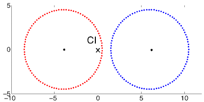
Figure 5: Two contours $z_{\pm s}$ of Eq. (32): the red contour ($z_{-s}$) encircles the CI point, and the blue contour ($z_{+s}$) does not. Parameters were set to $z_{c}=x_{c}+iy_{c}=1$, $d=10$, $r=9$.

Figure 5 shows that this choice generates two contours which are topologically different with respect to the CI point. Thus, the contour that encompasses the CI produces a change in the mixing angle $\theta$ [Eq. (7)] by $2\pi$, while moving along the other contour returns $\theta$ to its initial value (see Fig. 6).

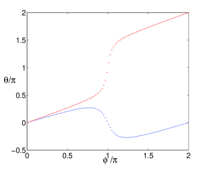
Figure 6: $\theta$-$\phi$ relation for the contours on Fig. 5: the red (blue) dots follow the contour that encircles (does not encircle) the CI point. Parameters of the Hamiltonian (1) are chosen so that $\theta={\rm arctan}(y/x)$

Adiabatic transport along these contours will lead to a sign change in all products of the electronic components $\ket{\psi_{\alpha^{\prime}}^{\rm adi}(\mathbf{R}_{c}-\mathbf{s}/2)}\bra{\psi_{\alpha}^{\rm adi}(\mathbf{R}_{c}+\mathbf{s}/2)}$ and, thus, this concludes our illustration of the double-valued character of the $f_{\alpha\alpha^{\prime}}(\mathbf{s};\mathbf{R}_{c})$ functions.

References

- Migani and Olivucci (2004) A. Migani and M. Olivucci, in Conical Intersection Electronic Structure, Dynamics and Spectroscopy, edited by W. Domcke, D. R. Yarkony, and H. Köppel (World Scientific, Singapore, 2004) p. 271.
- Yarkony (1996) D. R. Yarkony, Rev. Mod. Phys. 68, 985 (1996).
- Blancafort, Hunt, and Robb (2005) L. Blancafort, P. Hunt, and M. A. Robb, J. Am. Chem. Soc. 127, 3391 (2005).
- Blancafort et al. (2001) L. Blancafort, F. Jolibois, M. Olivucci, and M. A. Robb, J. Am. Chem. Soc. 123, 722 (2001).
- Izmaylov et al. (2011) A. F. Izmaylov, D. Mendive-Tapia, M. J. Bearpark, M. A. Robb, J. C. Tully, and M. J. Frisch, J. Chem. Phys. 135, 234106 (2011).
- Longuet-Higgins et al. (1958) H. C. Longuet-Higgins, U. Opik, M. H. L. Pryce, and R. A. Sack, Proc. R. Soc. A 244, 1 (1958).
- Berry (1984) M. V. Berry, Proc. R. Soc. A 392, 45 (1984).
- Simon (1983) B. Simon, Phys. Rev. Lett. 51, 2167 (1983).
- Ham (1987) F. S. Ham, Phys. Rev. Lett. 58, 725 (1987).
- Berry (1987) M. V. Berry, Proc. R. Soc. A 414, 31 (1987).
- Aitchison (1988) I. J. R. Aitchison, Phys. Scr. 1988, 12 (1988).
- Schön and Köppel (1994) J. Schön and H. Köppel, Chem. Phys. Lett. 231, 55 (1994).
- Schön and Köppel (1995) J. Schön and H. Köppel, J. Chem. Phys. 103, 9292 (1995).
- Ryabinkin and Izmaylov (2013) I. G. Ryabinkin and A. F. Izmaylov, Phys. Rev. Lett. 111, 220406 (2013).
- Joubert-Doriol, Ryabinkin, and Izmaylov (2013) L. Joubert-Doriol, I. G. Ryabinkin, and A. F. Izmaylov, J. Chem. Phys. (2013), in press, arXiv:1310.2929 .
- Cederbaum (2004) L. S. Cederbaum, in Conical Intersections, edited by W. Domcke, D. R. Yarkony, and H. Köppel (World Scientific, Singapore, 2004) pp. 3–40.
- Baer (1975) M. Baer, Chem. Phys. Lett. 35, 112 (1975).
- Köppel and Schubert (2006) H. Köppel and B. Schubert, Mol. Phys. 104, 1069 (2006).
- Van Voorhis et al. (2010) T. Van Voorhis, T. Kowalczyk, B. Kaduk, L.-P. Wang, C.-L. Cheng, and Q. Wu, Ann. Rev. Phys. Chem. 61, 149 (2010).
- Sirjoosingh and Hammes-Schiffer (2011) A. Sirjoosingh and S. Hammes-Schiffer, J. Chem. Theory Comput. 7, 2831 (2011).
- Yarkony (2012) D. R. Yarkony, Chem. Rev. 112, 481 (2012).
- Subotnik et al. (2009) J. E. Subotnik, R. J. Cave, R. P. Steele, and N. Shenvi, J. Chem. Phys. 130, 234102 (2009).
- Opalka and Domcke (2010) D. Opalka and W. Domcke, J. Chem. Phys. 132, 154108 (2010).
- Troisi and Orlandi (2003) A. Troisi and G. Orlandi, J. Chem. Phys. 118, 5356 (2003).
- Papas, Schuurman, and Yarkony (2008) B. N. Papas, M. S. Schuurman, and D. R. Yarkony, J. Chem. Phys. 129, 124104 (2008).
- Nakamura and Truhlar (2001) H. Nakamura and D. G. Truhlar, J. Chem. Phys. 115, 10353 (2001).
- Mead and Truhlar (1979) C. A. Mead and D. G. Truhlar, J. Chem. Phys. 70, 2284 (1979).
- Kendrick and Mead (1995) B. Kendrick and C. A. Mead, J. Chem. Phys. 102, 4160 (1995).
- Kendrick, Alden Mead, and Truhlar (2002) B. K. Kendrick, C. Alden Mead, and D. G. Truhlar, Chem. Phys. 277, 31 (2002).
- Kendrick (2003a) B. K. Kendrick, in Conical Intersections. Electronic Structure, Dynamics and Spectroscopy, Advanced Series in Physical Chemistry, Vol. 15, edited by W. Domcke, D. R. Yarkony, and H. Köppel (World Scientific, Singapore, 2003) Chap. 12, pp. 521–553.
- Kendrick and Pack (1996a) B. Kendrick and R. T. Pack, J. Chem. Phys. 104, 7475 (1996a).
- Kendrick and Pack (1996b) B. Kendrick and R. T. Pack, J. Chem. Phys. 104, 7502 (1996b).
- Kendrick (1997) B. Kendrick, Phys. Rev. Lett. 79, 2431 (1997).
- Kendrick (2003b) B. K. Kendrick, J. Phys. Chem. A 107, 6739 (2003b).
- Baer (1997) M. Baer, J. Chem. Phys. 107, 2694 (1997).
- Xu, Baer, and Varandas (2000) Z. Xu, M. Baer, and A. J. C. Varandas, J. Chem. Phys. 112, 2746 (2000).
- Kendrick, Mead, and Truhlar (1999) B. K. Kendrick, C. A. Mead, and D. G. Truhlar, J. Chem. Phys. 110, 7594 (1999).
- Kapral (2006) R. Kapral, Annual Review of Physical Chemistry 57, 129 (2006).
- Kelly and Kapral (2010) A. Kelly and R. Kapral, J. Chem. Phys. 133, 084502 (2010).
- Kapral and Ciccotti (1999) R. Kapral and G. Ciccotti, J. Chem. Phys. 110, 8919 (1999).
- Horenko et al. (2002) I. Horenko, C. Salzmann, B. Schmidt, and C. Schütte, J. Chem. Phys. 117, 11075 (2002).
- Ando and Santer (2003) K. Ando and M. Santer, J. Chem. Phys. 118, 10399 (2003).
- İmre et al. (1967) K. İmre, E. Özizmir, M. Rosenbaum, and P. F. Zweifel, J. Math. Phys. 8, 1097 (1967).
- Note (1) A more physically appealing derivation proceeds by scaling the equation so that an expansion of the Liouville operator in small parameter , where m and M are the characteristic masses of the quantum subsystem and bath DOF, can be carried out ( see Ref \rev@citealpnumKapral:1999/jcp/8919).
- Kernan, Ciccotti, and Kapral (2008) D. M. Kernan, G. Ciccotti, and R. Kapral, The Journal of Physical Chemistry B 112, 424 (2008).
- Ferretti et al. (1996) A. Ferretti, G. Granucci, A. Lami, M. Persico, and G. Villani, J. Chem. Phys. 104, 5517 (1996).