The number of killings in southern rural Norway, 1300–1569

Abstract

Three dual systems estimates are employed to study the number of killings in southern rural Norway in a period of slightly over 250 years. The first system is a set of five letters sent to each killer as part of the legal process. The second system is the mention of killings from all other contemporary sources. The posterior distributions derived suggest fewer such killings than rough demographic estimates.

and

1 Norwegian homicide law and the documentary evidence

This paper studies the number of killings in Norway in the period 1300–1569, that is, the last fifty years of Norway’s High Middle Age, through the Late Middle Ages, and a generation or so into the Early Modern Age. The extant written data about such killings, is of course, only a fraction of the documents issued.

Certain homicides (and some other crimes) were “noncompensation crimes” (ubotemal), which means that they, unless the king decided otherwise, were atoned for by capital punishment or outlawry and confiscation of the criminal’s property. Noncompensation homicides would, for instance, be the killing of a man in his own house, the killing of a kinsman, or a killing on a holy day. A study of the documents issued in such cases shows that King Magnus the Lawmender’s National Law of 1274 was systematically set aside in such cases, for good economic reasons. There would be no compensation to the victim’s next of kin, and it might even be a loss to the king’s district officer (sysselmann, the equivalent of an English sheriff) if he had to pay an executioner the equivalent of a craftsman’s monthly pay for decapitating a pennyless youngster. With, however, an economic atonement for the killing (botemal), the vicim’s heirs would get their compensation, and the king’s district officer would get the fine [strictly speaking, two fines, a recently introduced one for depriving the king of a subject (tegngilde) and an older one for the king’s pardon (fredkjop), similar to the continental Germanic fredus] nominally due to the king, which was about fifty percent of the normal compensation. In case of noncompensation killings the fine would be relatively higher, one regular fine for a killing, to which would be added another one for the killing of a brother, a second if it took place in his own house, and a third if it took place on a holy day. As we can see from some documents, family members would help to pay even though their legal obligation to do so had been abolished in 1260. The loss of a family member, cherished or not, would weaken the family. Some may have contributed in money or species, others may have guaranteed as securities as some documents show. Furthermore, there was some opportunity for haggling and the period before the compensation or fine was fully paid might on occasion be considerably longer than the year specified in the letter of pardon.

This process had five documents as its outcome. The killer, who was left at large and indeed might be said to be the prosecutor, had first to go to the King’s Chancellor in Oslo to get a protection letter (gridsbrev) which both gave him a temporary protection against avengers and also was an order to the king’s district officer to hear the case so as to find whether the killer had fulfilled the obligation of taking public responsibility for the killing and also whether he had sureties for the payment of compensation and fine. In accordance with this the district officer held a hearing with witnesses and the parties present and issued an evidence letter (provsbrev) summing up the relevant facts, including what might make this one or several ubotemal. With this provsbrev the killer had once more to travel to the King’s Chancellor who then issued a permanent pardon (landsvist, right to stay in the country) which also stated the amount to be paid in fine, and the condition that compensation and fine were to be paid within a year. As we can see, practice did at times give the killer several years respite before these sums were paid, but when paid they resulted in one receipt from the king’s district officer and one from the victim’s heirs. These five letters were all preserved in the killer’s archive as part of a farm archive together with deeds, inheritance divisions etc. until fire, wetness or some overly tidy daughter-in-law put an end to the existence of the large majority.

Supplementary material [Kadane and Næshagen (2013)] is an index of the documents that did survive, showing evidence of 337 killings in this time period. Of these, 194 are documented from the killer’s archive, 143 are only from other sources and 4 are mentioned both in the killer’s archive and in other sources. The other sources are quite varied, but include local officials, the King’s Chancellor, regional potentates, church officials, and private letters and diaries. The data used in this paper are summarized in Table 1.

Table 1: Two-way classification of records of killings

		Number of letters from killer’s archive
		0	1	2	3	4	5	Total
Mentioned in other sources?	No	$n$	$162$	$20$	5	3	0	$190+n$
	Yes	143	$3$	$0$	1	0	0	147
Total		$143+n$	$165$	$20$	6	3	0	$337+n$

The purpose is to find a distribution for $n$ and hence for $337+n$, the total number of killings in the period.

2 Demographic evidence about the number of killings

During this period Norway (like other European countries) underwent dramatic demographic changes. There is, furthermore, some disagreement about absolute numbers in given years during this period, but the most recent text book authors agree that when the plague first hit Norway in 1349 its population may have been 500,000 and perhaps slightly lower in the preceding half century. The recurrent plague epidemics reduced the population to its lowest point ca. 1450 to 1500, ca 200,000 or perhaps less [Moseng et al. (2007), pages 233–236, 294 and 295]. After this population started growing again and, in spite of recurrent epidemics, grew to 440,000 in the 1660s, the first really reliable assessment. These estimates concern Norway as it was then, before the country had lost almost ten percent of its territory and population due to Danish military misadventures. The data used here are, for the sake of comparison, only taken from present-day Norwegian territory, so about ten percent should be deducted from population estimates.

With two exceptions there is no conspicuous geographic bias in the data. Telemark, which both in the Middle Ages and later had a reputation for violence, is very well represented in these data. Due to the cases where the scene of the homicide is geographically localized, or that of the person paying for receiving compensation or fine, or their provenience (come to an archive from a rural district) is, and the fact that family archives are preserved in rural districts, as farm archives while similar urban archives are unknown, we can be fairly sure that scarcely any of these documents had an urban origin—which means that they reflect the situation in the countryside, not in the much more violent cities and towns. This may account for the discrepancy between the homicide estimates for the mid-sixteenth century (10–15 per 100,000) made from another type of data (accounts of fines and confiscations) by Næshagen (2005), and the somewhat lower estimates this study yields. Only about 3 percent of the population lived in the three larger cities, Bergen, Trondheim and Oslo, but their population showed an extreme inclination to homicide. Thus, Bergen, Norway’s largest and most heterogenous city, with a population of 6,000 had from 1562 to 1571 a homicide rate of 83 per 100,000 [Sandnes (1990), pages 72–74]. Thus, with these rural data one should expect a somewhat lower estimate than Næshagen’s 10 to 15 per 100,000 from the mid-sixteenth century which includes cities (2005).

Central Norway (Tr$\o$ndelag) and Northern Norway with, respectively, 13 and 11 percent of the population [Dyrvik (1979), page 18] seem not to be represented among these documents. Judging from the mid-sixteenth-century lists of fines and confiscations, homicides may have been rarer in Central Norway than in the rest of the country, while Northern Norway does not distinguish itself in any way [Næshagen (2005), page 416], and later data support the conclusion about Central Norway [Sandnes (1990), page 79].

So supposing that the population of Norway as it was then was 500,000 in the period from 1300 to 1350, and roughly 200,000 in the period from 1350 to 1569, we must deduct 10% to account for the territory lost. This yields 450,000 in 1300 to 1350, and 180,000 for the later period. Additionally, we deduct 24% (13% in Central Norway, 11% in Northern Norway) for rural areas not covered, and another 3% for the cities, yielding a deduction of 27%. Thus, we estimate rural southern Norway to have had a population of 330,000 in the period from 1300 to 1350, and 130,000 from 1350 to 1569. It should be emphasized that these are rough estimates only.

The next set of estimates concerns the rate of killings. Accepting the estimates from somewhat later of 10 to 15 per hundred thousand per year overall, but a much higher rate (83 per hundred thousand) for the 3% of the urban population suggests a rate of 8 to 13 per hundred thousand per year in rural southern Norway.

Applied to the 50 year period before the plague and the 219 years after the plague, this yields a range of 3600 to 5850 for the number of killings in rural southern Norway during the period in question.

3 Models of the data

Problems of missing data are ubiquitous; indeed, every parameter not known with certainty can be regarded as “missing data” in some sense. In biostatistics, survival analysis can be regarded as a method for dealing with missing time-of-death data for patients still alive. But these problems are especially acute in history, geology, the interpretation of fossils, astronomy and archeology. In one instance, Kadane and Hastorf (1988), the authors assumed known preservation probabilities for different kinds of burnt seeds in an archeological site in Peru.

While the methods used here bear a relationship with problems of estimating the number of species [see Bunge and Fitzpatrick (1993) for a review], the more closely related literature is that of dual systems estimators, growing out of the early work of Petersen (1896) and Lincoln (1930), and applied to the problem of census coverage by Wolter (1986).

A. Simple dual systems

The simplest treatment of data of this kind is to amalgamate all mentions in the killer’s archive together, resulting in the following $2\times 2$ table.

Table 2: Reduced data

		Killer’s archive?
		No	Yes	Total
Mentioned in other sources?	No	$n$	190	$190+n$
	Yes	143	4	147
Total		$143+n$	194	$337+n$

To establish notation for this case, let the numbers in Table 2 be represented as shown in Table 3.

=295pt Killer’s archive? No Yes Total Mentioned in other sources? No $n_{00}$ $n_{01}$ $n_{0+}$ Yes $n_{10}$ $n_{11}$ $n_{1+}$ Total $n_{+0}$ $n_{+1}$ $n_{++}$ []Note: $n_{00}=n$.

Table 3: General notation for Table 2

The data can be taken to be multinomial, with probabilities $p_{ij}$, and hence likelihood

$$L=\pmatrix{n_{++}\cr n_{00},n_{01},n_{10},n_{11}}\mathop{\prod_{i=0,1}}_{j=0,1}p^{n_{ij}}_{ij}.$$ (1)

A key assumption is that of independence, which would mean that whether a killing is known from the preservation of a letter from the killer’s archive has no bearing on whether it is known from the other sources. In this application, such an assumption seems entirely reasonable. So if $p$ is the probability a killing is mentioned in other sources and $q$ is the probability a killing is known from at least one letter from the killer’s archive, the assumption of independence can be written as

$$p_{ij}=p^{i}\overline{p}{}^{\overline{i}}q^{j}\overline{q}{}^{\overline{j}},\qquad i=0,1;j=0,1,$$ (2)

where $\overline{x}=1-x$.

Substituting (2) into (1) yields

$$L=\pmatrix{n_{++}\cr n_{00},n_{01},n_{10},n_{11}}p^{n_{1+}}\overline{p}{}^{n_{0+}}q^{n_{+1}}\overline{q}{}^{n_{+0}}.$$ (3)

The parameters $p,q$ and $n$ are all that matter here, and $n$ is the parameter of interest. Any reasonable prior distribution (i.e., one that is not strongly opinionated) for $p$ and $q$ will lead to the same inference, given the values of $n_{0+},n_{1+},n_{+0}$ and $n_{+1}$ in this data set. Hence, we accept independent uniform priors for $p$ and $q$. In view of the material in Section 2, the prior of interest on the total number of killings, $n+337$, is uniform $(337,5850)$. However, for the first computation reported here we use a much broader uniform prior on $n$ in order to show the uncertainty inherent in the likelihood.

Using the well-known integration result,

$$\int^{1}_{0}x^{n}(1-x)^{m}\,dx = B(n+1,m+1)=\frac{\Gamma(n+1)\Gamma(m+1)}{\Gamma(n+m+2)}$$

$$= \frac{n!m!}{(n+m+1)!},$$

the integrated likelihood is

$$\pmatrix{n_{++}\cr n_{00},n_{01},n_{10},n_{11}}\frac{n_{1+}!n_{0+}!n_{+1}!n_{+0}!}{[(n_{++}+1)!]^{2}}.$$ (5)

Now $n_{01},n_{10},n_{11},n_{+1}$ and $n_{1+}$ do not depend on $n$. Hence, these factors do not matter for the integrated likelihood, yielding an integrated likelihood proportional to

$$\frac{(n_{0+})!(n_{+0})!}{n_{00}!(n_{++}+1)(n_{++}+1)!}=\frac{(n+190)!(n+143)!}{n!(n+338)(n+338)!}.$$ (6)

Figure 1 plots, as a probability distribution, the quantity $n+337$, the total number of killings. Implicitly the prior on $n$ used in this calculation is uniform with an upper bound of at least 25,000, which is much higher than we find credible. Nonetheless, for display purposes, we show it.

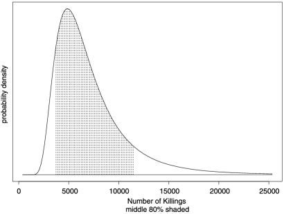
Figure 1: Simple dual systems integrated likelihood.

The quantiles of the data in Figure 1 are reported in Table 4. Together Figure 1 and Table 4 suggest substantial uncertainty about the total number of killings; the middle 80% of the distribution lies between 3337 and 10,837, a gap of 7500 killings; the median of the distribution is 5837.

Table 4: Quantiles for Figure 1

Quantile	3337	3837	4337	4837	5837	6337	7337	8337	10,837
Probability	0.1	0.2	0.3	0.4	0.5	0.6	0.7	0.8	0.9

This suggests the desirability of making more use of the data in Table 1, and in particular the data on the number of letters found in each killer’s archive.

B. Dual systems binomial model

To do so, we now establish general notation for Table 1, in Table 5.

Let $\mathbf{n}=(n_{00},n_{01},n_{02},\ldots,n_{05},n_{10},n_{11},\ldots,n_{15})$ and $\mathbf{n}!=\prod^{5}_{i=0}\prod^{1}_{j=0}n_{ij}!$.

Then the multinomial likelihood can be written as

$$L=\frac{n_{++}!}{\mathbf{n}!}\mathop{\prod_{i=0,1}}_{j=0,\ldots,5}p^{n_{ij}}_{ij}.$$ (7)

Again imposing independence, we have

$$p_{ij}=r_{j}s^{i}\overline{s}{}^{\overline{i}},\qquad j=0,\ldots,5;i=0,1,$$ (8)

where $r_{j}$ is the probability of $j$ surviving letters in the archive and $s$ is the probability of being mentioned in other sources.

Table 5: Notation for Table 1

		Number of letters in killer’s archive
		0	1	2	3	4	5	Total
Mentioned in other sources?	No	$n_{00}$	$n_{01}$	$n_{02}$	$n_{03}$	$n_{04}$	$n_{05}$	$n_{0+}$
	Yes	$n_{10}$	$n_{11}$	$n_{12}$	$n_{13}$	$n_{14}$	$n_{15}$	$n_{1+}$
Total		$n_{+0}$	$n_{+1}$	$n_{+2}$	$n_{+3}$	$n_{+4}$	$n_{+5}$	$n_{++}$

Substituting (8) into (7), we obtain

$$L=\frac{n_{++}!}{\mathbf{n}!}\prod^{5}_{j=0}r^{n+j}_{j}s^{n_{1+}}\overline{s}{}^{n_{0+}}.$$ (9)

A simple model to impose on $\mathbf{r}=(r_{o},r_{1},\ldots,r_{5})$ is binomial $(5,p)$, where $p$ is here the probability that each letter in a killer’s archive survives (this assumption is revisited in subsection C, ahead). With the binomial assumption,

$$r_{j}=\pmatrix{5\cr j}p^{j}\overline{p}{}^{5-j},\qquad j=0,\ldots,5.$$ (10)

Then

$$\prod^{5}_{j=0}r^{n+j}_{j}=\prod^{5}_{j=0}\pmatrix{5\cr j,5-j}^{n_{+j}}p^{\sum^{5}_{j=0}jn_{+j}}\overline{p}{}^{\sum^{5}_{j=0}(5-j)n_{+j}}.$$ (11)

Let $S_{1}=\sum^{5}_{j=0}jn_{+j}$. Then $\sum^{5}_{j=0}(5-j)n_{+j}=5n_{++}-S_{1}$.

Hence,

$$\prod^{5}_{j=0}r_{j}^{n_{+j}}=\prod^{5}_{j=0}\pmatrix{5\cr j,5-j}^{n_{+j}}p^{S_{1}}\overline{p}{}^{5n_{++}-S_{1}}.$$ (12)

The first term on the right can be written for our data as

$$\prod^{5}_{j=0}\pmatrix{5\cr j,5-j}^{n_{+j}}$$

$$\qquad=\biggl{(}\frac{5!}{0!5!}\biggr{)}^{n+143}\biggl{(}\frac{5!}{1!4!}\biggr{)}^{165}\biggl{(}\frac{5!}{2!3!}\biggr{)}^{20}\biggl{(}\frac{5!}{3!2!}\biggr{)}^{6}\biggl{(}\frac{5!}{4!1!}\biggr{)}^{3}\biggl{(}\frac{5!}{0!5!}\biggr{)}^{0}.$$

Only the first term has an exponent that depends on a parameter, and that term is 1 raised to a power, so the entire product is constant with respect to the parameters, and can be dropped. Similarly, in the terms for $\mathbf{n}!$ only the first, $n!$, depends on the parameters, and the others can be dropped:

$$L\propto\frac{(n_{++})!}{n!}p^{S_{1}}\overline{p}{}^{5n_{++}-S_{1}}s^{n_{1+}}\overline{s}{}^{n_{0+}}.$$ (14)

Again, using (3) and independent uniform distributions on $p$ and $s$, the integrated likelihood for $n$ is

$$\frac{(n_{++})!}{n!}\frac{(S_{1})!(5n_{++}-S_{1})!}{(5n_{++}+1)!}\frac{(n_{1+})!(n_{0+})!}{(n_{++}+1)!}$$

(15)

$$\qquad=\frac{S_{1}!(5n_{++}-S_{1})!(n_{1+})!(n_{0+})!}{n!(5n_{++}+1)!(n_{++}+1)}.$$

Finally, $S_{1}$ and $n_{1+}$ also do not depend on $n$, so those terms can be dropped as well, yielding the integrated likelihood proportional to

$$\frac{(5n_{++}-S_{1})!(n_{0+})!}{n!(5n_{++}+1)!(n_{++}+1)}.$$ (16)

Figure 2 plots the posterior distribution for $n+337$ whose quantiles are given in Table 6. Here the median is 1155.

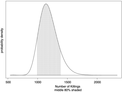
Figure 2: Binomial dual systems posterior distribution. Note that Figure 1 has a wider scale of the number of killings.

Table 6: Quantiles for dual systems posterior distribution under the binomial model

Quantile	978	1037	1076	1116	1155	1195	1234	1293	1372
Probability	0.1	0.2	0.3	0.4	0.5	0.6	0.7	0.8	0.9

Thus, this model suggests remarkably fewer killings than those suggested by the simple dual systems estimate reported in Figure 1 and Table 6.

C. Com-binomial model

The binomial model implies that the survival of a document from a killer’s archive is an event independent of the survival of other documents from the same killer’s archive. Since all five letters are addressed to the same person (the killer), it is likely that they would tend to be stored together. Hence, it seems prudent to expand the model to allow for positive correlation among the events of survival of letters addressed to the same killer. [A referee suggests that an overly tidy daughter-in-law may have kept only one letter, leading to negative correlation. While that may have happened in a few instances, we think that joint physical destruction (fire and water) is far more likely, and hence expect positive correlation in the survival event of documents from a killer’s archive.]

One model that allows for such correlation is the com-binomial distribution [Shmueli et al. (2004)]. The pdf for this distribution is given by

$$\quad P\{X=j|p,\nu\}=\frac{p^{j}(1-p)^{m-j}{m\choose j,m-j}^{\nu}}{\sum^{m}_{k=0}p^{k}(1-p)^{m-k}{m\choose k,m-k}^{\nu}},\qquad j=0,1,\ldots,m.$$ (17)

When $\nu=1$, this distribution reduces to the binomial distribution, and hence to independence of survival of the documents sent to a given killer. For $\nu>1$, the survival would be negatively correlated. For $\nu<1$, the survival would be positively correlated. In this application, the latter is expected. As $\nu\rightarrow\infty$, the probability would become concentrated on a single point. As $\nu\rightarrow-\infty$, it would become concentrated on 0 and $m$.

Because this distribution is unfamiliar, it is perhaps useful to look at some examples, displayed in Figure 3 for the case $m=5$, which is the value of $m$ in this application. In this figure, looking across rows, as $\nu$ increases, the probability tends to concentrate on a single point (except at $p=1/2$, where symmetry leads to two dominant points, 2 and 3).

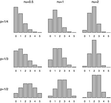
Figure 3: Com-binomial distribution for various values of $p$ and $nu$.

As alluded to above, values of $\nu$ above 1 do not make sense in this application. Therefore, the analysis to be presented imposes the condition $\nu\leq 1$ as a hard constraint, by using a prior that put zero probability in the space $\nu>1$.

To incorporate the com-binomial distribution into the model, $r_{j}$ in (10) is replaced by the expression in (17). This yields the likelihood

$$L = \frac{n_{++}!}{\mathbf{n}!}s^{n_{1+}}\overline{s}{}^{n_{0+}}\prod^{5}_{j=0}r_{j}^{n_{+j}}$$

$$= \frac{n_{++}!}{\mathbf{n}!}s^{n_{1+}}\overline{s}{}^{n_{0+}}\prod^{5}_{j=0}\biggl{[}\frac{p^{j}(1-p)^{m-j}{m\choose j,m-j}^{\nu}}{\sum^{m}_{k=0}p^{k}(1-p)^{m-k}{m\choose k,m-k}^{\nu}}\biggr{]}^{n_{+j}}.$$

It is convenient to divide the numerator and denominator in the product term by the factor $(1-p)^{m}(m!)^{\nu}$, yielding

$$\frac{p^{j}(1-p)^{m-j}{m\choose j,m-j}^{\nu}}{\sum^{m}_{k=0}p^{k}(1-p)^{m-k}{m\choose k,m-k}^{\nu}}=\frac{\theta^{j}/[j!(m-j)!]^{\nu}}{\sum^{5}_{k=0}\theta^{k}/[k!(m-k)!]^{\nu}},$$ (19)

where $\theta=p/(1-p)$.

It is further convenient to rewrite (19) as follows:

$$\theta^{j}\bigg{/}\Biggl{\{}\bigl{[}j!(m-j)!\bigr{]}^{\nu}\Biggl{(}\sum^{5}_{k=0}\theta^{k}/\bigl{[}k!(m-k)!\bigr{]}^{\nu}\Biggr{)}\Biggr{\}}$$

$$\qquad=e^{j\log\theta-\nu\log[j!(m-j)!]}/Z(\theta,\nu)$$ (20)

$$\eqntext{\mbox{where }\displaystyle Z(\theta,\nu)=\sum^{5}_{k=0}\theta^{k}/\bigl{[}k!(m-k)!\bigr{]}^{\nu}.}$$ (21)

Substituting (3) into (3) yields

$$L=\frac{n_{++}!}{\mathbf{n}!}s^{n_{1+}}\overline{s}{}^{n_{0+}}e^{s_{1}\log\theta-s_{2}\nu}/\bigl{(}Z(\theta,\nu)\bigr{)}^{n_{++}},$$ (22)

where $s_{1}=\sum^{5}_{j=1}jn_{+j}$ and $s_{2}=\sum^{5}_{j=0}n_{+j}\log(j!(5-j)!)$.

Once again $s$ can be integrated with respect to a uniform prior, yielding the integrated likelihood

$$\frac{n_{++}!}{\mathbf{n}!}\frac{(n_{1+})!(n_{0+})!}{(n_{++}+1)!}e^{s_{1}\log\theta-s_{2}\nu}/Z(\theta,\nu)^{n_{++}}.$$ (23)

Finally, factors not involving $\theta,\nu$ and $n$ can be eliminated, yielding

$$\frac{(n_{0+})!}{n!(n_{++}+1)}e^{s_{1}\log\theta-s_{2}\nu}Z(\theta,\nu)^{-n_{++}}.$$ (24)

In order to have results comparable to those in Figure 2, proper account must be taken of the transformation from $p$ to $\theta$. The differentials are related by

$$dp=\frac{d\theta}{(1+\theta)^{2}},$$ (25)

so $p$ uniform on $(0,1)$ is equivalent to $\theta$ having the density $1/(1+\theta)^{2}$ on $(0,\infty)$. Thus, the form of likelihood used here is (24) multiplied by (25), that is,

$$\frac{(n_{0+})!}{(n_{++}+1)n!}e^{s_{1}\log\theta-s_{2}\nu}\frac{Z(\theta,\nu)^{-n_{++}}}{(1+\theta)^{2}}.$$ (26)

Using a grid method to integrate (26) with respect to $\theta$ and $\nu$ yields the posterior distribution in Figure 4, with quantiles given in Table 7. The median for this model is 1143, about the same as for the binomial model.

The results of the com-binomial in Figure 4 are very similar to those of the binomial in Figure 2. The reason for this is that the likelihood for $\nu$ strongly indicates a preference for $\nu=1$. Glancing back at the data in Table 1, the data are strongly piled up at 0 and $1$ letters from a killer’s archive; there are no killings at all for which all five letters have survived. Therefore, the data looks much more like it would at $\nu=\infty$, which makes no substantive sense in this problem. Given that the hard constraint $\nu\leq 1$ has been imposed, the integrated posterior puts most weight on the largest $\nu$ permitted, that is, $\nu=1$; the results therefore resemble those of the binomial model reported in Figure 2. While the generalization afforded by the com-binomial did not lead to a substantially different integrated likelihood, it was important to see whether positive correlation in the survival of letters sent to the killer was a dominant feature of the data. This turned out not to be the case.

4 Conclusion

An assumption underlying our model is that every killing resulted in the five letters being sent to the killer. It is possible that this is not true, and possible that the propensity to send the requisite letters varied by geography. It is also possible that some geographical areas were more prone to document destruction by fire, flood, etc., and such areas might be those less carefully administered. We leave these possibilities for further exploration.

This paper presents three analyses of the number of killings in rural Norway during the period in question. The first (Table 4 and Figure 1) used only the presence or absence of a mention in the killer’s archive, and found huge uncertainty in the number of killings. The latter two, reported, respectively, in Table 6 and Figure 2, and in Table 7 and Figure 4, are so similar that substantively they are the same. The distribution reported indicates that perhaps rural Norway was more peaceful in this period than had previously been thought.

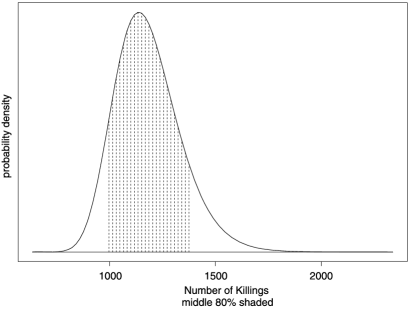
Figure 4: Com-binomial posterior distribution. Note that Figure 1 has a wider scale for the number of killings.

Table 7: Quantiles for dual systems integrated likelihood under the com-binomial model

Quantile	959	1021	1051	1113	1143	1174	1235	1265	1357
Probability	0.1	0.2	0.3	0.4	0.5	0.6	0.7	0.8	0.9

References

- Bunge and Fitzpatrick (1993) {barticle}[author] \bauthor\bsnmBunge, \bfnmJ.\binitsJ. and \bauthor\bsnmFitzpatrick, \bfnmM.\binitsM. (\byear1993). \btitleEstimating the Number of Species: A Review. \bjournalJ. Amer. Statist. Assoc. \bvolume88 \bpages364–373. \bptokimsref \endbibitem
- Dyrvik (1979) {bincollection}[author] \bauthor\bsnmDyrvik, \bfnmStâle\binitsS. (\byear1979). \btitleJordbruk og folketal 1500–1720. In \bbooktitleNorsk Okonomisk Historie 1500–1970, Band 1 1500–1850 (\beditor\bfnmS.\binitsS. \bsnmDyrvik, \beditor\bfnmA. B.\binitsA. B. \bsnmFossen, \beditor\bfnmT.\binitsT. \bsnmGrønlie, \beditor\bfnmE.\binitsE. \bsnmHovland, \beditor\bfnmH.\binitsH. \bsnmNordvik and \beditor\bfnmS.\binitsS. \bsnmTveite, eds.). \bpublisherUniversitetsforlaget, \blocationBergen. \bptokimsref \endbibitem
- Kadane and Hastorf (1988) {binproceedings}[author] \bauthor\bsnmKadane, \bfnmJ. B.\binitsJ. B. and \bauthor\bsnmHastorf, \bfnmC.\binitsC. (\byear1988). \btitleBayesian Paleoethnobotany. In \bbooktitleBayesian Statistics III (\beditor\bfnmD. V.\binitsD. V. \bsnmLindley, \beditor\bfnmJ.\binitsJ. \bsnmBernardo, \beditor\bfnmM.\binitsM. \bsnmDeGroot and \beditor\bfnmA. F. M.\binitsA. F. M. \bsnmSmith, eds.) \bpages243–259. \bpublisherOxford Univ. Press, \baddressOxford. \bptokimsref \endbibitem
- Kadane and Næshagen (2013) {bmisc}[author] \bauthor\bsnmKadane, \bfnmJ. B.\binitsJ. B. and \bauthor\bsnmNæshagen, \bfnmF. L.\binitsF. L. (\byear2013). \bhowpublishedSupplement to “The number of killings in southern rural Norway, 1300–1569.” DOI:\doiurl10.1214/12-AOAS612SUPP. \bptokimsref \endbibitem
- Lincoln (1930) {barticle}[author] \bauthor\bsnmLincoln, \bfnmF. C.\binitsF. C. (\byear1930). \btitleCalculating waterfowl abundance on the basis of banding returns. \bjournalUnited State Department of Agriculture Circular \bvolume118 \bpages1–4. \bptokimsref \endbibitem
- Moseng et al. (2007) {bbook}[author] \bauthor\bsnmMoseng, \bfnmO. G.\binitsO. G., \bauthor\bsnmOpsahl, \bfnmE.\binitsE., \bauthor\bsnmPettersen, \bfnmG. I.\binitsG. I. and \bauthor\bsnmSandmo, \bfnmE.\binitsE. (\byear2007). \btitleNorsk Historie 750–1537, 2. Utgave. \bpublisherUniversitetsforlaget, \blocationOslo. \bptokimsref \endbibitem
- Næshagen (2005) {barticle}[author] \bauthor\bsnmNæshagen, \bfnmF. L.\binitsF. L. (\byear2005). \btitleDen kriminelle voldens U-kurve fra femtenhundretall til natid. (The U-curve of criminal violence from the sixteenth century to the present.) \bjournalHistorisk Tidsskrift \bvolume84 \bpages411–427. \bptokimsref \endbibitem
- Petersen (1896) {barticle}[author] \bauthor\bsnmPetersen, \bfnmC. G. J.\binitsC. G. J. (\byear1896). \btitleThe yearly immigration of young plaice into the Limfjord from the German sea. \bjournalReport of the Danish Biological Station (1895) \bvolume6 \bpages5–84. \bptokimsref \endbibitem
- Sandnes (1990) {bbook}[author] \bauthor\bsnmSandnes, \bfnmJ.\binitsJ. (\byear1990). \btitleKniven, ølet og aeren. \bpublisherUniversitetsforlaget, \blocationOslo. \bptokimsref \endbibitem
- Shmueli et al. (2004) {barticle}[author] \bauthor\bsnmShmueli, \bfnmG.\binitsG., \bauthor\bsnmMinka, \bfnmT. P.\binitsT. P., \bauthor\bsnmKadane, \bfnmJ. B.\binitsJ. B., \bauthor\bsnmBorle, \bfnmS.\binitsS. and \bauthor\bsnmBoatwright, \bfnmP.\binitsP. (\byear2004). \btitleA useful distribution for fitting discrete data: Revival of the COM-Poisson. \bjournalJ. R. Stat. Soc. Ser. C. Appl. Stat. \bvolume54 \bpages127–142. \bptokimsref \endbibitem
- Wolter (1986) {barticle}[mr] \bauthor\bsnmWolter, \bfnmKirk M.\binitsK. M. (\byear1986). \btitleSome coverage error models for census data. \bjournalJ. Amer. Statist. Assoc. \bvolume81 \bpages338–346. \bidissn=0162-1459, mr=0845875 \bptokimsref \endbibitem