Discussions on the crossover property within the Nambu–Jona-Lasinio model

Abstract

In this paper, chiral symmetry breaking and its restoration are investigated in the mean field approximation of Nambu–Jona-Lasinio model. A first-order phase transition exists at low temperature, but is smeared out at high temperature. We discuss the rationality of using susceptibilities as the criteria to determine the crossover region as well as the critical point. Based on our results, it is found that to define a critical band instead of an exclusive line in this region might be a more suitable choice.

PACS Number(s): 12.39.-x, 25.75.Nq, 12.39.Fe

I Introduction

Quantum chromodynamics (QCD) Gross and Wilczek (1973); Politzer (1973) is often viewed as the basic theory of strong interaction. In the process of large momentum transfer, the coupling constant is small (which is the so-called asymptotic freedom phenomenon Politzer (1974)), so that the scattering process can be treated perturbatively with much success. However, in the process of small momentum transfer, the coupling constant becomes large so that problems have to be treated with various nonperturbative methods.

The Nambu–Jona-Lasinio model (NJL) Nambu and Jona-Lasinio (1961a, b) is an effective model of QCD which was proposed in 1961. In this model, interaction terms are treated as four-body interactions, meanwhile, the Lagrangian is constructed such that the basic symmetries of QCD that are observed in nature are part and parcel of it. In particular, the NJL model exhibits the feature of dynamical chiral symmetry breaking Nambu (1960); Goldstone (1961), which is responsible for the dynamical mass generation from bare quarks. Nevertheless, there are also two shortcomings of the NJL model; namely, it is neither confining nor renormalizable. As for the former one, the NJL model is expected to work well in the region of intermediate length between the asymptotic freedom and confinement regions and applied to the properties for which confinement is expected not to be essential. For the latter shortcoming, a momentum cutoff is often introduced to avoid the ultraviolet divergence.

At high temperature and/or high density, the features of confinement and chiral symmetry breaking are expected to be destroyed. The effective quark mass and the pion mass may change discontinuously at certain point of temperature and density, which corresponds to the chiral phase transition. In the chiral limit, the quark condensate can be regarded as an order parameter of this phase transition, however, how to define the quark condensate beyond the chiral limit from first principles of QCD is still an open problem Maris et al. (1998), and so there is no rigorous order parameter right now. Instead, the effective quark mass $M$ (or the quark condensate beyond chiral limit, although it has no rigorous definition) and various susceptibilities are often used as the criteria to determine the critical point of chiral phase transition Asakawa and Yazaki (1989); He et al. (2009); Shi et al. (2010); Jiang et al. (2011); Li et al. (2013). In this work, we try to study the critical point of phase transition in the case of finite temperature and finite chemical potential by means of several susceptibilities in the NJL model.

The rest of this paper is organized as follows. In Sec. ii@ the NJL model is briefly reviewed, and we will treat problems in the mean field approximation of this model. In Sec. iii@ we present the results of M.Asakawa and K.Yazaki Asakawa and Yazaki (1989) on the chiral phase transition, and question the rationality of their criterion for the critical point in the crossover region. In Sec. iv@, several susceptibilities, which are expected to be the criteria for the critical point, are calculated. Finally, in Sec. v@ we will summarize our results and give the conclusions.

II The Nambu–Jona-Lasinio Model

As an important effective theory, NJL model is widely used in many fields, for example, Refs Zhao et al. (2008); Andersen and Kyllingstad (2010); Lenzi et al. (2010); Abuki et al. (2010); Chernodub (2011); Carignano and Buballa (2012); Buballa and Carignano (2013); Cui et al. (2013) are some recent representative applications. The Lagrangian of the NJL model Asakawa and Yazaki (1989) is (in this paper, we take the number of flavors $N_{f}=2$, and the number of colors $N_{c}=3$.)

$$\mathscr{L}_{\text{NJL}}=\bar{\psi}({\mathrm{i}}\not{\partial}-m)\psi+{\mathrm{g}}[(\bar{\psi}\psi)^{2}+(\bar{\psi}{\mathrm{i}}\gamma_{5}{\boldsymbol{\tau}}\psi)^{2}],$$ (1)

where $m$ is the current quark mass for two flavors, $g$ is a coupling constant with the dimension of mass^-2, and the flavor and color indices are suppressed.

The thermal expectation value of an operator $\Theta$ is denoted as

$$\langle\!\langle\Theta\rangle\!\rangle=\frac{\mathrm{Tr}\,\Theta\,{\mathrm{e}}^{-\beta(\mathscr{H}-\mu\mathscr{N}})}{\mathrm{Tr}\,{\mathrm{e}}^{-\beta(\mathscr{H}-\mu\mathscr{N})}}.$$ (2)

Then, we apply the mean field approximation Kunihiro and Hatsuda (1984); Hatsuda and Kunihiro (1985) to $\bar{\psi}\psi,\bar{\psi}\gamma_{0}\psi$ in the original and Fierz-transformed interaction terms, while other terms vanish. Hence the mean field interaction terms can be written as

$$\mathscr{L}_{\text{MFint}}= \frac{4N_{c}+1}{2N_{c}}{\mathrm{g}}\langle\!\langle\bar{\psi}\psi\rangle\!\rangle\bar{\psi}\psi+\frac{\mathrm{g}}{N_{c}}\langle\!\langle\bar{\psi}\gamma_{0}\psi\rangle\!\rangle\bar{\psi}\gamma_{0}\psi$$ (3)

$$-\frac{4N_{c}+1}{4N_{c}}{\mathrm{g}}\langle\!\langle\bar{\psi}\psi\rangle\!\rangle^{2}+\frac{\mathrm{g}}{2N_{c}}\langle\!\langle\bar{\psi}\gamma_{0}\psi\rangle\!\rangle^{2},$$

and the Hamiltonian density is

$$\mathscr{H}= -{\mathrm{i}}\bar{\psi}{\boldsymbol{\gamma}}{\boldsymbol{\cdot}}{\boldsymbol{\nabla}}\psi+m\bar{\psi}\psi-\mathscr{L}_{\text{MFint}}$$ (4)

$$= -{\mathrm{i}}\bar{\psi}{\boldsymbol{\gamma}}{\boldsymbol{\cdot}}{\boldsymbol{\nabla}}\psi+M\bar{\psi}\psi$$

$$+\frac{\mathrm{g}}{N_{c}}\sigma_{2}\mathscr{N}+G\sigma_{1}^{2}-\frac{\mathrm{g}}{2N_{c}}\sigma_{2}^{2},$$

where $G=\frac{4N_{c}+1}{4N_{c}}{\mathrm{g}}$ is the renormalized coupling constant, $\mathscr{N}=\bar{\psi}\gamma_{0}\psi=\psi^{\dagger}\psi$ is the operator for the quark number density and $M$ is the effective quark mass

$$M=m-2G\sigma_{1},$$ (5)

$\sigma_{1}$ and $\sigma_{2}$ are defined, respectively, as follows:

$$\sigma_{1}=\langle\!\langle\bar{\psi}\psi\rangle\!\rangle,$$ (6)

$$\sigma_{2}=\langle\!\langle\psi^{\dagger}\psi\rangle\!\rangle,$$ (7)

where $\sigma_{1}$ is the quark condensate which is often viewed as the order parameter for chiral phase transition in the chiral limit.

The Hamiltonian density in (4) describes a system of free quarks with mass $M$ and chemical potential $\mu_{r}$ given by

$$\mu_{r}=\mu-\frac{{\mathrm{g}}}{N_{c}}\sigma_{2},$$ (8)

where $\mu$ is the bare chemical potential.

Now we use the formalism of the thermal Green function in the real time Dolan and Jackiw (1974) to determine $\sigma_{1}$ and $\sigma_{2}$ self-consistently at finite temperature and chemical potential. The thermal Green function of a free fermion at temperature $T$ and chemical potential $\mu$ written in momentum space is as follows:

$$G(p;T,\mu)= (\not{p}+M)\bigg{[}\frac{1}{p^{2}-M^{2}+{\mathrm{i}}\varepsilon}+2\pi{\mathrm{i}}\delta(p^{2}-M^{2})$$ (9)

$$\times\{\theta(p^{0})n(\boldsymbol{p},\mu)+\theta(-p^{0})m(\boldsymbol{p},\mu)\}\bigg{]},$$

with

$$n(\boldsymbol{p},\mu)=\frac{1}{1+\exp{[\beta(E-\mu)]}},$$ (10)

$$m(\boldsymbol{p},\mu)=\frac{1}{1+\exp{[\beta(E+\mu)]}},$$ (11)

$E_{p}=\sqrt{M^{2}+{\boldsymbol{p}}^{2}}$ and $\beta=1/T$. Using this propagator, $\sigma_{1}$ and $\sigma_{2}$ can be calculated out Asakawa and Yazaki (1989). The results are written as

$$\begin{split}\sigma_{1}=-M\frac{N_{c}N_{F}}{\pi^{2}}\!\int_{0}^{\Lambda}\!\frac{p^{2}}{E}\big{\{}1-n(\boldsymbol{p},\mu_{r})-m(\boldsymbol{p},\mu_{r})\big{\}}{\mathrm{d}}p\\ \end{split}$$ (12)

$$\begin{split}\sigma_{2}=\frac{N_{c}N_{F}}{\pi^{2}}\int_{0}^{\Lambda}p^{2}\big{\{}n(\boldsymbol{p},\mu_{r})-m(\boldsymbol{p},\mu_{r})\big{\}}{\mathrm{d}}p,\end{split}$$ (13)

where $\Lambda$ is a momentum cutoff, which is introduced to avoid the ultraviolet divergence mentioned above. For convenience we will use the noncovariant three-momentum cutoff scheme  Bernard (1986).

Now Eqs. (5),(8),(12) and (13) form a set of self-consistent equations. By solving these equations self-consistently, one can obtain the effective quark mass for each temperature and chemical potential. In this paper, we will employ the widely accepted parameter set according to Hatsuda and Kunihiro Hatsuda and Kunihiro (1994): $m=5.5~{}{\mathrm{MeV}},\Lambda=631~{}{\mathrm{MeV}},{\mathrm{g}}=5.074\times 10^{-6}~{}{\mathrm{MeV}}^{-2}$, which yields pion mass $M_{\pi}=138~{}{\mathrm{MeV}}$, pion decay constant $f_{\pi}=93.1~{}{\mathrm{MeV}}$, and quark condensate ${\langle\!\langle\bar{\psi}\psi\rangle\!\rangle}^{1/3}=-331~{}{\mathrm{MeV}}$.

III chiral restoration and the phase diagram

In the case of zero temperature and finite chemical potential, the effective quark mass $M$ obtained numerically using the iterative method is shown in Fig. 1.

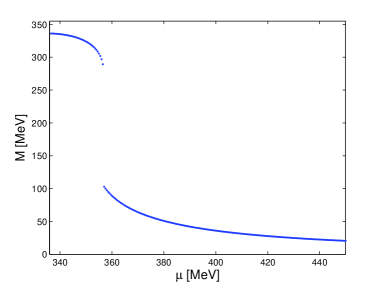
Figure 1: (color online). The effective quark mass $M$ at $T$=0

As can be seen from Fig. 1, there is a discontinuity of $M$ at some certain chemical potential, the behavior of the quark condensate $\sigma_{1}$ is the same as that of $M$ [see Eq. (5)], we can conclude that if $M$ can serve as an order parameter in this case, a first-order phase transition occurs at a coexistence chemical potential and zero temperature. One defect, although it does not affect our subsequent discussions on the crossover property and the quantitative results in the first order transition, should be pointed out. As many literatures, e.g., Sasaki et al. (2008); Pinto et al. (2012) show, the gap equation has more than one solution including an unstable solution and a metastable solution in the vicinity of the coexistence chemical potential in the first-order phase transition region. In order to select the solutions corresponding to stable points, it is wiser to find the smaller minima of the effective thermodynamical potential. The phase transition line can be located at the chemical potential where the effective thermodynamical potential has two degenerate minima. Then, with the increase of temperature, the two degenerate minima of the effective thermodynamical potential will get closer, i.e., the discontinuity of $M$ becomes small, and at last the discontinuity of $M$ comes to disappear at a critical temperature $T_{c}$, which means the first-order phase transition is smeared out. It is worthwhile to mention that the equations which the critical temperature $T_{c}$ should satisfy can be obtained by other techniques such as Landau’s expansion or the method presented by Contrera et al.  Contrera et al. (2010). Avancini et al.. also provide other alternative to determine the first order line, the critical endpoint as well as the crossover region Avancini et al. (2012).

At supercritical temperature $T>T_{c}$, there is no evident critical line which can be defined in the $T-\mu$ plane. However, the thermodynamical properties change rather sharply across a band in the plane, thus it is necessary to draw the phase diagram neglecting the smearing. M.Asakawa and K.Yazaki Asakawa and Yazaki (1989) pointed out that there is a region where the effective quark mass $M$ changes very rapidly with temperature and chemical potential, and when the first-order phase transition is observed ($T<T_{c}$), $M$ jumps from a value larger than or around $\frac{1}{2}M_{0}$ to a value smaller than or around $\frac{1}{2}M_{0}$, where $M_{0}$ is denoted as the effective quark mass at $T=0$ and $\mu=0$. At $T=T_{c}$, $M$ changes most rapidly at the point where $M\simeq\frac{1}{2}M_{0}$. Considering that the critical line should be continuous at $T=T_{c}$, they artificially define the critical points as the points where the effective quark mass takes the same value as that at $T=T_{c}$, i.e., $\frac{1}{2}M_{0}$. According to this criterion, the phase transition diagram is plotted in Fig. 2, where the “+” lines stand for the first-order phase transition lines and the “*” lines stand for the smooth transition regions as defined above.

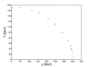
Figure 2: (color online). Phase transition line in the $T-\mu$ plane

Considering that the artificially defined critical point is aimed to describe the rapid change of thermodynamical properties, more convincing criteria for the critical point are the extremum of susceptibilities, such as the chiral susceptibility and the quark number susceptibility Jiang et al. (2011); He et al. (2009). We will move on to discuss these in the next section of this paper.

IV various susceptibilities and the crossover region

Now let us introduce the definitions of four kinds of susceptibilities: the chiral susceptibility $\chi_{s}$, the quark number susceptibility $\chi_{q}$, the vector-scalar susceptibility $\chi_{vs}$, and another auxiliary susceptibility $\chi_{m}$. For mathematical convenience we first introduce these susceptibilities in the free quark gas case (the interaction terms in the Lagrangian is zero, i. e., $\mathscr{L}_{int}=0$) Kunihiro (2000), where $M$ and $\mu_{r}$ are reduced to $m$ and $\mu$, which are independent quantities. Denoting them with the superscript ⁽⁰⁾, their definitions and expressions are as follows:

$$\begin{split}\chi_{s}^{(0)}\equiv&-\frac{\partial\langle\!\langle\bar{\psi}\psi\rangle\!\rangle_{f}}{\partial m}\\ =&\frac{N_{c}N_{f}}{\pi^{2}}\int_{0}^{\Lambda}\bigg{[}\frac{m^{2}p^{2}\beta}{E^{2}}g(\mu)+\frac{p^{4}}{E^{3}}f(\mu)\bigg{]}{\mathrm{d}}p,\end{split}$$ (14)

$$\begin{split}\chi_{q}^{(0)}\equiv&\frac{\partial\langle\!\langle\psi^{\dagger}\psi\rangle\!\rangle_{f}}{\partial\mu}=\frac{N_{c}N_{f}}{\pi^{2}}\int_{0}^{\Lambda}p^{2}\beta g(\mu){\mathrm{d}}p,\end{split}$$ (15)

$$\begin{split}\chi_{vs}^{(0)}\equiv&\frac{\partial\langle\!\langle\bar{\psi}\psi\rangle\!\rangle_{f}}{\partial\mu}=\frac{N_{c}N_{f}}{\pi^{2}}\int_{0}^{\Lambda}\frac{mp^{2}\beta}{E}h(\mu){\mathrm{d}}p,\end{split}$$ (16)

$$\begin{split}\chi_{m}^{(0)}\equiv-\frac{\partial\langle\!\langle\psi^{\dagger}\psi\rangle\!\rangle_{f}}{\partial m}=\chi_{vs}^{(0)},\end{split}$$ (17)

where $g(\mu)+h(\mu)=2n(\mu)(1-n(\mu))$, $g(\mu)-h(\mu)=2m(\mu)(1-m(\mu))$, $f(\mu)=1-n(\mu)-m(\mu)$, the subscript $f$ represents the free quark gas systems. It should be noted that $\chi_{m}^{(0)}$ and $\chi_{vs}^{(0)}$ have the same analytical expression, which is reasonable from the viewpoint of statistical mechanics:

$$\chi_{m}^{(0)}=\chi_{vs}^{(0)}=\frac{T}{V}\frac{\partial^{2}}{\partial m\partial\mu}\ln Z_{f},$$ (18)

where $Z_{f}$ is the QCD partition function in the free quark gas case.

In the interacting case, $M$ and $\mu_{r}$ are no longer independent. These susceptibilities are coupled with each other as follows:

$$\begin{split}\chi_{s}\equiv&-\frac{\partial\langle\!\langle\bar{\psi}\psi\rangle\!\rangle}{\partial m}\\ =&\chi_{s}^{(0)}(\mu_{r})(1+2G\chi_{s})-\frac{{\mathrm{g}}}{N_{c}}\chi_{vs}^{(0)}(\mu_{r})\chi_{m},\end{split}$$ (19)

$$\begin{split}\chi_{q}\equiv&\frac{\partial\langle\!\langle\psi^{\dagger}\psi\rangle\!\rangle}{\partial\mu}\\ =&2G\chi_{vs}^{(0)}(\mu_{r})\chi_{vs}+\chi_{q}^{(0)}(\mu_{r})(1-\frac{{\mathrm{g}}}{N_{c}}\chi_{q}),\end{split}$$ (20)

$$\begin{split}\chi_{vs}\equiv&\frac{\partial\langle\!\langle\bar{\psi}\psi\rangle\!\rangle}{\partial\mu}\\ =&2G\chi_{s}^{(0)}(\mu_{r})\chi_{vs}+\chi_{vs}^{(0)}(\mu_{r})(1-\frac{{\mathrm{g}}}{N_{c}}\chi_{q}),\end{split}$$ (21)

$$\begin{split}\chi_{m}\equiv&-\frac{\partial\langle\!\langle\psi^{\dagger}\psi\rangle\!\rangle}{\partial m}\\ =&\chi_{m}^{(0)}(\mu_{r})(1+2G\chi_{s})-\frac{{\mathrm{g}}}{N_{c}}\chi_{q}^{(0)}(\mu_{r})\chi_{m}.\end{split}$$ (22)

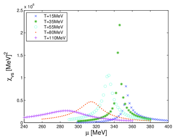
Figure 3: (color online). $\chi_{vs}$ at different $\mu$ and $T$

Using the iterative method, we can obtain the numerical results of these susceptibilities. For example, the vector-scalar susceptibility is the response of the effective quark mass ($M=m-2G\langle\!\langle\bar{\psi}\psi\rangle\!\rangle$) to the chemical potential $\mu$, and its result is shown in Fig. 3.

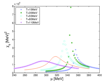
Figure 4: (color online). $\chi_{s}$ at different $\mu$ and $T$

It can be seen that, when $T$ is smaller than the critical value $T_{c}=35$ MeV, there always exists a convergent discontinuity of $\chi_{vs}$, corresponding to a first-order phase transition; when $T=T_{c}$, $\chi_{vs}$ displays a sharp and narrow divergent peak, which implies a second-order phase transition, or in other words, here is a critical end point; when $T>T_{c}$, the discontinuity disappears and a rather broad peak of finite height is shown, corresponding to the crossover region. We pick the peak of the susceptibility as the artificial critical point to draw the phase diagram, which would produce little change on Fig. 2.

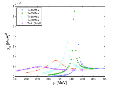
Figure 5: (color online). $\chi_{q}$ at different $\mu$ and $T$

Comparing these with the results of chiral susceptibility $\chi_{s}$ and quark number susceptibility $\chi_{q}$, shown in Fig. 4 and 5, respectively, we can conclude that at low temperature, the first-order phase transition occurs at almost the same chemical potential, while in the crossover region, the artificially defined critical point tends to occur at different chemical potentials as the temperature increases.

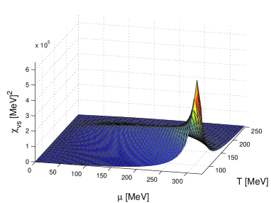
Figure 6: (color online). Vector-scalar susceptibility $\chi_{vs}$ in the crossover region

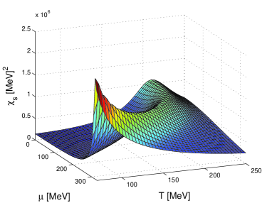
Figure 7: (color online). Chiral susceptibility $\chi_{s}$ in the crossover region

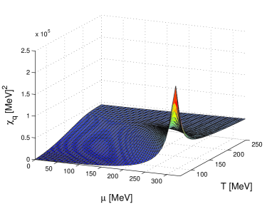
Figure 8: (color online). Quark number susceptibility $\chi_{q}$ in the crossover region

The calculated results of $\chi_{vs}$, $\chi_{s}$, and $\chi_{q}$ in the crossover region are shown in Figs. 6-8, respectively. $\chi_{vs}$ and $\chi_{m}$ give the same numerical results for the reason mentioned above. We can find that they exhibit different behaviors: the chiral susceptibility $\chi_{s}$ exhibits an obvious band, so it is convincing to define the peak of $\chi_{s}$ as the artificial critical point; in the high $T$ and/or low $\mu$ region, the vector-scalar susceptibility $\chi_{vs}$ tends to vanish; while the global shape of the quark number susceptibility $\chi_{q}$ is just similar to the ones of $\chi_{s}$ and $\chi_{vs}$, but it is nonvanishing in the high $T$ and/or high $\mu$ region whose behavior is closely linked to the quark number density. This result is consistent with K. Fukushima’s result obtained using the PNJL model Fukushima (2008). Therefore, $\chi_{q}$ cannot describe the crossover property well in the high $T$ and/or high $\mu$ region.

It is very interesting and meaningful to compare the results of these susceptibilities with that of the thermal susceptibility $\chi_{T}=\partial\langle\!\langle\bar{\psi}\psi\rangle\!\rangle/\partial T$ which is widely used in many recent literatures, e.g., Morita et al. (2011); Skokov (2012). For mathematical convenience, we define $\chi_{n}=\partial\langle\!\langle\psi^{\dagger}\psi\rangle\!\rangle/\partial T$. By the same process employed above, we obtain a set of coupled equations for $\chi_{T}$ and $\chi_{n}$ as follows:

$$\begin{split}\chi_{T}\equiv&\frac{\partial\langle\!\langle\bar{\psi}\psi\rangle\!\rangle}{\partial T}\\ &=\frac{\partial\langle\!\langle\bar{\psi}\psi\rangle\!\rangle}{\partial M}\frac{\partial M}{\partial T}+\frac{\partial\langle\!\langle\bar{\psi}\psi\rangle\!\rangle}{\partial\mu_{r}}\frac{\partial\mu_{r}}{\partial T}+\big{(}\frac{\partial\langle\!\langle\bar{\psi}\psi\rangle\!\rangle}{\partial T}\big{)}_{M,\mu_{r}}\\ =&2G\chi_{s}^{(0)}(\mu_{r})\chi_{T}-\frac{{\mathrm{g}}}{N_{c}}\chi_{vs}^{(0)}(\mu_{r})\chi_{n}\\ &+M\beta\chi_{q}^{(0)}(\mu_{r})-\mu_{r}\beta\chi_{m}^{(0)}(\mu_{r}),\end{split}$$ (23)

$$\begin{split}\chi_{n}\equiv&\frac{\partial\langle\!\langle\psi^{\dagger}\psi\rangle\!\rangle}{\partial T}\\ =&\frac{\partial\langle\!\langle\psi^{\dagger}\psi\rangle\!\rangle}{\partial M}\frac{\partial M}{\partial T}+\frac{\partial\langle\!\langle\psi^{\dagger}\psi\rangle\!\rangle}{\partial\mu_{r}}\frac{\partial\mu_{r}}{\partial T}+\big{(}\frac{\partial\langle\!\langle\psi^{\dagger}\psi\rangle\!\rangle}{\partial T}\big{)}_{M,\mu_{r}}\\ =&2G\chi_{m}^{(0)}(\mu_{r})\chi_{T}-\frac{{\mathrm{g}}}{N_{c}}\chi_{q}^{(0)}(\mu_{r})\chi_{n}\\ &-\mu_{r}\beta\chi_{q}^{(0)}(\mu_{r})+\frac{N_{c}N_{f}}{\pi^{2}}\int_{0}^{\Lambda}p^{2}E\beta^{2}h(\mu){\mathrm{d}}p.\end{split}$$ (24)

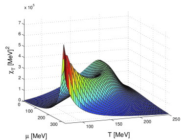
Figure 9: (color online). Thermal susceptibility $\chi_{T}$ in the crossover region

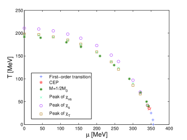
Figure 10: (color online). Phase diagram obtained according to different criteria

The behavior of $\chi_{T}$ in the crossover region is shown in Fig.9, which is very similar to that of $\chi_{s}$. The comparison between them will be shown in the phase diagram.

The phase diagram is given in Fig. 10 according to different criteria for the critical point in the crossover region as follows: the peaks of $\chi_{vs}$, $\chi_{T}$, and $\chi_{s}$. We compare our results with that of M.Asakawa and K.Yazaki. The line given by the peak of $\chi_{vs}$ is almost the same as that of M.Asakawa and K.Yazaki, while the lines given by the peaks of $\chi_{T}$ and $\chi_{s}$ both display a shift as compared with that of M.Asakawa and K.Yazaki. In the $\mu=0$ case, the peak of $\chi_{vs}$ appears at $T=196$ MeV, while the peaks of $\chi_{T}$ and $\chi_{s}$ appear at $T=198$ MeV and $T=211$ MeV, respectively. Here we do not give the results of $\chi_{q}$ due to the reason mentioned above. Therefore, it is hard to define the critical line in the crossover region, and a critical band might be a more suitable choice.

V summary and conclusion

In this paper we study the chiral phase transition at finite temperature and chemical potential and calculate several susceptibilities in the mean field approximation using the Nambu–Jona-Lasinio model.

We discuss the rationality of using susceptibilities as the criteria to determine the crossover region as well as the critical point. In the low temperature region, the first-order phase transition is found to be at almost the same chemical potential for different susceptibilities, which is due to the fact that these susceptibilities are coupled with each other in their mathematical form; at sufficiently high temperature, the first-order phase transition is smeared out, and the results of different susceptibilities imply the uncertainty in the position of the artificially defined critical point in the $T-\mu$ plane. So, it is more suitable to define a critical band rather than an exclusive line in the crossover region.