Christine Davies

School of Physics and Astronomy
The University of Glasgow, Glasgow, UK

The determination of the charm quark mass is now possible to 1% from QCD, with lattice QCD pushing the error down below 1%. I will describe the ingredients of this approach and how it can achieve this accuracy. Results for quark mass ratios, $m_{c}/m_{s}$ and $m_{b}/m_{c}$, can also be determined to 1% from lattice QCD, allowing accuracy for the heavy quark masses to be leveraged into the light quark sector. I will discuss the prospects for, and importance of, improving results in future calculations.

PRESENTED AT

The 6^th International Workshop on Charm Physics
(CHARM 2013)
Manchester, UK, 31 August – 4 September, 2013

1 Introduction

Quark masses are important parameters of the Standard Model but cannot be obtained directly from experiment because quarks are never seen as free particles. Instead they must be inferred from experimental results for hadrons. The accuracy of the determination of quark masses is a topical issue because of the need to test the couplings to quarks of the newly discovered Higgs boson [1, 2, 3]. The Standard Model rate for decay of a Higgs to $c\overline{c}$ or $b\overline{b}$ is sensitive to the charm/bottom quark mass. The quark mass parameter in the QCD Lagrangian is a well-defined quark mass but it is scheme- and scale-dependent (i.e. it ‘runs’). Lattice QCD has a clear advantage here when determining quark masses, because the calculations start from the QCD Lagrangian and the parameters of that Lagrangian are readily tuned. To do this, quark mass parameters are chosen, at a given value of the lattice spacing, to reproduce the experimental result for the mass of a hadron containing that quark. This gives the quark mass in the lattice scheme very accurately. However, most calculations (such as those for Higgs decay) need quark masses in a continuum renormalisation scheme such as $\overline{MS}$. A key source of error is then the conversion from the lattice quark mass to the $\overline{MS}$ scheme. Continuum methods for determining the quark mass rely on evaluating a quantity from experiment that can also be calculated accurately in QCD perturbation theory in terms of, say, the $\overline{MS}$ quark mass. As discussed below, accurate values for $c$ and $b$ masses can be obtained in this way using experimental results derived from $\sigma(e^{+}e^{-}\rightarrow\mathrm{hadrons})$ [4, 5]. Very similar methods can be used with lattice QCD results [6, 7] effectively to convert the lattice quark mass to the $\overline{MS}$ scheme, and it is these methods that give the most accurate results from lattice QCD also. I will describe both methods and their results in Section 3 but first give a brief introduction to lattice QCD.

2 Lattice QCD Calculations

Lattice QCD calculations proceed by a standard recipe [8] which starts with setting up a 4-d space-time volume, discretised into a set of points with lattice spacing, $a$. Configurations of gluon fields (one SU(3) matrix for every link joining two points on the lattice) are generated by Monte Carlo methods according to the probability distribution required in the QCD Feynman Path Integral. This probability distribution is $\exp(-S_{QCD})$ where $S_{QCD}$ is the sum over the configuration of the Lagrangian of QCD. The probability distribution is for the gluon fields but, in modern lattice QCD calculations, it includes the effect of sea quarks that are generated in the ‘soup’ of particles that make up the QCD vacuum. The parameters of QCD enter in specifying the QCD Lagrangian. These are the bare coupling constant and the quark masses. It is important to realise that the lattice spacing is not specified at this point - it must be determined from calculations performed on these configurations.

Figure 1: Left: a $c\overline{c}$ meson correlation function in QCD and also the charm quark vacuum polarisation. Charm quark propagators connect the two currents, $J$. Right: The correlation function for a $c\overline{c}$ pseudoscalar meson multiplied by $e^{Mt}$ (where $M$ is the fitted ground-state mass) and plotted against time $t/a$ in lattice units. The ground-state clearly dominates the correlation function at large $t$. The statistical errors from the lattice calculation are shown, but are so small as to be barely visible.

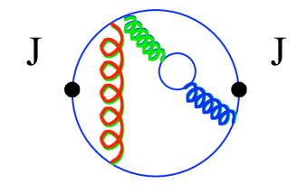
Once sets of gluon field configurations have been generated, we can calculate quark propagators on them by solving the Dirac equation. In this equation the gluon field appears in the covariant derivative term and the quark mass is a parameter. Combining a quark and antiquark propagator together (making sure the colours match at both ends and the spins are combined appropriately) makes a meson correlation function. This is the amplitude to create a meson at one point and destroy it at some other point. Averaging the meson correlation functions obtained over all the gluon field configurations generated gives us a Monte Carlo estimate of the result for this amplitude from the QCD Feynman Path Integral. The meson correlation function is illustrated in Figure 1 (left). It shows the meson being created and destroyed by an operator $J$, which is implemented when the quark propagators are tied together. At intermediate points the charm quark and antiquark interact with each other via the gluon fields and sea quarks in the background configuration. The meson mass is determined by fitting the average meson correlation function as a function of time on the lattice (we sum the end-points over $x$, $y$, $z$, at fixed $t$ to project onto zero spatial momentum for the meson). Because we are working with Euclidean time, the expected behaviour at large times is as an exponential (rather than the more normal phase factor):

$$\langle 0|J^{{\dagger}}(t_{0}+t)J(t_{0})|0\rangle\equiv G(t)\stackrel{{\scriptstyle t\rightarrow\infty}}{{=}}Ae^{-Mt}=Ae^{-Ma\times(t/a)}.$$ (1)

The exponent is the mass of the lowest mass meson with the quantum numbers of the operator, $J$. The last piece of the equation above shows that, in fitting the correlation function in terms of time on the lattice $t/a$ (i.e. the number of lattice spacings between two points in time) we will be able to determine the mass of the meson also in lattice units, i.e. the dimensionless combination $Ma$. We need to obtain a value for $a$ in order to convert this to physical, GeV, units. This is done by using another hadron mass (preferably one that is rather insensitive to quark masses) and setting the lattice result equal to the experimental value [9]. Quantities used for this include the radial excitation energy in the $\Upsilon$ system [10] and the $\pi$ decay constant [11].

Figure 2: Left: the gold-plated heavy meson spectrum from lattice QCD (points) compared to experiment [9] (red lines). Light cyan crosses denote those masses used to fix the parameters of QCD; green squares indicate postdictions and dark blue circles indicate predictions ahead of experiment. Recent lattice results are from [10, 15, 16, 17] Right: Moments of vector current-current correlators from lattice QCD plotted against the square of the lattice spacing [17]. The dashed line shows the continuum extrapolation. The black points at $a=0$ correspond to values extracted from experiment for the charm contribution to $R_{e^{+}e^{-}}$ [5].

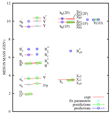
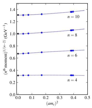
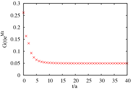
Figure 1 (right) shows the correlator for the $c\overline{c}$ pseudoscalar meson, for which the lowest mass meson is the $\eta_{c}$. The quantity plotted is $G(t)e^{Mt}$, where $Ma$ is the value obtained for the ground-state mass from a fit to the correlator. This value is $Ma=1.32724(3)$ which corresponds to 2.982(3) GeV at this value of the lattice spacing ($a=0.08784(9)\mathrm{fm}\equiv 1/2.2466(23)\,\mathrm{GeV}^{-1}$). This shows how accurately the $\eta_{c}$ mass can be obtained. The calculation required fixing the charm quark mass, also in lattice units. The value here, using the Highly Improved Staggered formalism [12] for the $c$ quarks, was $m_{c}a=0.432$. The 0.1% accuracy obtainable on the $\eta_{c}$ mass, means that the lattice $c$ quark mass (on which it is linearly dependent) can be tuned to a similar level of accuracy [13]. Figure 1 also demonstrates the behaviour of the correlator. At large values of $t$ it is dominated by the ground-state $\eta_{c}$, so that $G(t)e^{Mt}$ is a constant. At shorter times this is not true. Then higher mass states (for example, radial excitations) contribute and their masses can be determined with a careful calculation (as discussed elsewhere in these Proceedings [14]). This region merges seamlessly with the region where the correlator is controlled by perturbative QCD. It is the short time region that we use to match the lattice $m_{c}$ to that in a continuum scheme, as described in the next Section. The $\eta_{c}$ is only one of a range of meson masses that can be accurately determined from lattice QCD. Figure 2 shows a summary plot of the spectrum of ‘gold-plated’ mesons containing $c$ and $b$ quarks from lattice QCD and its comparison with experiment. A gold-plated meson is one that has no strong Zweig-allowed decay mode and so has a very narrow width. The accuracy of many of these masses from lattice QCD is now at the few MeV level where we need to worry about and estimate electromagnetic effects missing from our pure QCD calculations [13]. The agreement with experiment is excellent, providing a stringent test of QCD. Indeed, some of the masses were predicted ahead of experiment. Handling $c$ and $b$ quarks presents some difficulties in lattice QCD because they are relatively heavy. When the Dirac equation is discretised onto a lattice of points the covariant derivative is replaced by a finite difference and this is only correct up to systematic errors of $\mathcal{O}(a^{2})$. The question is, what sets the scale for these errors? For hadrons made of light quarks, this will typically be the scale of QCD, i.e. a few hundred MeV. For heavy quarks it can be the quark mass itself. For $c$ quarks, $m_{c}a$ is around 0.4 for typical lattice spacing values of around 0.1 fm. An error of $\mathcal{O}([m_{c}a]^{2})$ could then be of size 20%. Working with ‘improved’ discretisations raises the power of $ma$ in the error and improves the situation. For the Highly Improved Staggered Quark (HISQ) action [12] that is used here, the leading errors are $\alpha_{s}^{2}(m_{c}a)^{2}$ and $(m_{c}a)^{4}$, which give errors of a few % at $a=$ 0.1fm. It is important to obtain results at multiple values of the lattice spacing and extrapolate to $a=0$ to remove the discretisation errors. This extrapolation is relatively benign if a highly improved action is used and therefore the error in the final result from this extrapolation is small.

3 The current-current correlator method

The production of a $c\overline{c}$ pair occurs directly in the real world in $e^{+}e^{-}$ collisions. Figure 1 (left) can also illustrate this case by representing the ‘heavy quark vacuum polarisation’. Then $J$ is the $c\overline{c}$ vector current which couples to the photon produced in $e^{+}e^{-}$. If we cut the diagram down the centre we expose a lot of quark-antiquark pairs and gluons produced from the original $c\overline{c}$ pair which, by unitarity, will end up as hadrons in the final state. Information about the charm quark vacuum polarisation can then be extracted from $\sigma(e^{+}e^{-}\rightarrow\mathrm{hadrons})$ if we can isolate the piece of the cross-section that corresponds to $c$ quark pair production. Because $R_{e^{+}e^{-}}=\sigma(e^{+}e^{-}\rightarrow\mathrm{hadrons})/\sigma_{\mathrm{point}}$ has step-like behaviour as a function of centre-of-mass energy $\sqrt{s}$ with well-separated heavy quark regions, this can be done using a mixture of theory and experiment. The contribution from $u$, $d$ and $s$ quarks can be calculated and subtracted, as illustrated in Figure 3 from [5]. The basic tree-level QED calculation from textbooks [18] gives $R_{e^{+}e^{-}}=3\sum_{i}Q^{2}_{q_{i}}$ for $i$ flavours of quarks with $Q_{q_{i}}$ the electric charge of that quark flavour in units of $e$, ignoring quark mass effects. QCD corrections can be incorporated that are impressively known up to and including $\alpha_{s}^{3}$ terms [19]. The ‘natural’ scale for $\alpha_{s}$ is $\sqrt{s}$, so this gives an accurate picture for $R$ in the region of a few GeV (below the charm threshold), and the agreement with experiment is good. Higher order electromagnetic contributions can be determined and they are very small; effects from the $Z$ are negligible.

Figure 3: $R_{e^{+}e^{-}}$ as a function of centre-of-mass energy, $\sqrt{s}$, around the charm threshold region. The solid line, with uncertainties given by the dashed lines, gives the prediction in perturbative QCD below and above the charm threshold. Figure from [5].

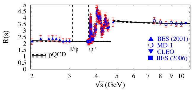
The $c$ quark contribution to $R_{e^{+}e^{-}}$, $R_{c}(s)$, then has pieces corresponding to the charm resonances (modelled as narrow peaks using the experimental information about each state), the charm threshold region (obtained from experiment after subtraction for $u$, $d$, and $s$ quarks) and the higher $s$ region above the charm threshold obtained from perturbation theory, again compared to experiment [5] or directly from experiment [20]. Around the charm threshold region $R_{c}(s)$ is very sensitive to the charm quark mass and this can be used to determine $m_{c}$. The determination of $m_{c}$ uses analyticity properties to obtain the (dispersion) relationship between $s$-inverse moments of $R_{c}(s)$ and $q^{2}$-derivative moments of the charm quark vacuum polarisation function evaluated at $q^{2}=0$ [18]:

$$\mathcal{M}_{k,expt}\equiv\int\frac{ds}{s^{k+1}}R_{c}(s)=\mathcal{M}_{k,th}\equiv\left.\frac{12\pi^{2}}{k!}\left(\frac{d}{dq^{2}}\right)^{k}\Pi_{c}(q^{2})\right|_{q^{2}=0}.$$ (2)

$\mathcal{M}_{k,expt}$ is evaluated from $R_{c}(s)$ and the numbers are shown as the black points on the right-hand plot of Figure 1 (where $n=2k+2$). Errors are 1% or better. The contribution from the resonances dominates. $\mathcal{M}_{k,th}$, i.e. the $q^{2}$ derivatives of $\Pi_{c}$, needs evaluation of the behaviour of $\Pi_{c}$ at small $q^{2}$, i.e. in a very different kinematic region to that for $R_{c}(s)$. For heavy quarks, $q^{2}=0$ is well below the threshold to produce real quarks (so the $c$ quarks in Figure 1 (left) would be virtual). The expansion of $\Pi_{c}$ about $q^{2}=0$ can then be evaluated in QCD perturbation theory and the derivatives obtained, giving for the vector current case

$$\mathcal{M}_{k,th}=Q_{c}^{2}\frac{9}{4}C_{k,V}\left(\frac{1}{4m_{c}^{2}}\right)^{k};\,\,C_{k,V}=C_{k,V}^{{0}}+\alpha_{s}C_{k,V}^{(1)}+\ldots.$$ (3)

This exposes clearly the sensitivity of $\mathcal{M}_{k}$ to the $c$ quark mass. $m_{c}$ in the equation above can be, for example, the $c$ quark mass in the $\overline{MS}$ scheme evaulated at the scale $\mu$. The perturbative series, $C_{k}$, is a power series expansion in $\alpha_{s}$. Its coefficients will reflect the scheme and scale chosen for $m_{c}$ so that the final result (to all orders) for $\mathcal{M}_{k}$ is scheme and scale invariant, and has the value obtained from experiment via $R_{c}$ in equation 2. The ‘natural’ scale for $\alpha_{s}$ here is $2m_{c}$, which is large enough for reasonably good control of the perturbative expansion. In fact, the QCD perturbation theory for $C_{k}$ has reached an extremely impressive level of calculation. Values for $C_{k}^{(3)}$ are known for the first few values of $k$, which corresponds to NNNLO [21, 22, 23]. Small values of $k$, 1 to 4, are preferred because larger values of $k$, although more sensitive to $m_{c}$, start to receive significant contributions from operators such as the gluon condensate which increase the uncertainty. Matching $\mathcal{M}_{k,th}$, with an input value of $\alpha_{s}$, to $\mathcal{M}_{k,expt}$ described above, Chetyrkin et al [5] obtain, in the $\overline{MS}$ scheme with number of flavours, $n_{f}=4$, $m_{c}(m_{c})$ = 1.279(13) GeV. This is obtained from using the lowest moment, $k=1$, in equation 3. The error is dominated by the experimental error in $R_{c}(s)$ and by the uncertainty taken in the value of $\alpha_{s}$ (3 times the current PDG uncertainty [9]). The uncertainty coming from unknown higher order terms in the perturbation theory is estimated in the standard way by varying the scale, $\mu$, at which $\alpha_{s}$ is evaluated (varying the coefficients $C_{k,V}$ appropriately). The central value used here is 3 GeV, which is the same as the scale used for the central value of $m_{c}$ (subsequently iteratively run to the scale of $m_{c}$). The variation taken is $\pm$ 1 GeV [5]. Perturbative error estimates are always somewhat subjective and these have been criticised in [20] as being too small, in particular pointing out that larger $\mu$ dependence can be seen when the $\mu$ in $\alpha_{s}$ and that in $m_{c}$ are decoupled. In the lattice QCD analysis described below we use the same perturbation theory but take a somewhat different approach to the perturbative errors, estimating directly the effect on $m_{c}$ of missing higher order terms using a Bayesian analysis. We are also able to fit multiple moments simultaneously and extract at the same time a value for $\alpha_{s}$. These features improve the accuracy with which $m_{c}$ can be determined. They require the use of pseudoscalar current-current correlators which are not accessible from experiment but, as discussed in Section 2, can be calculated very accurately in lattice QCD.

Figure 4: Time moments of pseudoscalar $c\overline{c}$ correlators calculated in lattice QCD as a function of the square of the lattice spacing [7]. The result extrapolated to $a=0$ can be used with continuum QCD perturbation theory to determine the $c$ quark mass in the $\overline{MS}$ scheme.

In lattice QCD we can substitute for $M_{k,expt}$ values of $\mathcal{M}_{k,latt}$ obtained by taking time-moments of the $c\overline{c}$ meson correlation functions described in Section 2. The correlation functions (at zero spatial momentum) are the Fourier transform from energy to time-space of the charm quark vacuum polarisation function. Thus $q^{2}$-derivative moments become (squared) time-moments and we use [6]

$$G_{n}=\sum_{t}(t/a)^{n}G(t);\,\,n=2k+2.$$ (4)

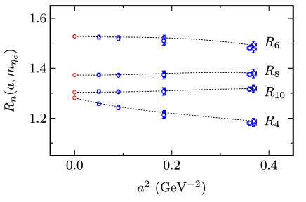
$G(t)$ is a meson correlation function averaged over gluon field configurations, as in equation 1. To compare to the continuum QCD perturbation theory of equation 3 we need to extrapolate $G_{n}$ to $a=0$ to obtain a continuum value. Thus we have to define $G(t)$ to be well-defined in that limit. For the HISQ formalism used here we have a PCAC relation (as in continuum QCD) that enables us to define an absolutely normalised pseudoscalar current operator: $J=(am_{c})\overline{c}\gamma_{5}c$ and we use this to create and destroy pseudoscalar $c\overline{c}$ states in our correlation function. To perform the analysis [6, 7] we calculate meson correlation functions at multiple values of the lattice spacing, fixing $am_{c}$ at each value of $a$ to be the value which gives the correct $\eta_{c}$ mass from the long-time behaviour of the correlator. We then calculate the time-moments as above for $n=$ 4, 6, 8 and 10 (corresponding to $k=$ 1, 2, 3 and 4 in equation 3). Taking time-moments emphasises the small, but non-zero, $t$ region of the correlation function since it is falling approximately exponentially (see Figure 1 right). Having a result for each moment at each value of $a$ then allows us to extrapolate to the continuum limit. The result for doing this for $c$ quarks is shown in Figure 4. To reduce discretisation errors we have actually plotted and extrapolated the ratio of $G_{n}$ to its value in the absence of gluon fields, $G_{n}^{(0)}$ (readily calculated by simply omitting the coupling to gluons in the Dirac equation). In fact we take:

$$R_{n,latt}=G_{4}/G_{4}^{(0)},\,n=4;\,\,R_{n,latt}=\frac{aM_{\eta_{c}}}{2am_{c}}\left(\frac{G_{n}}{G_{n}^{(0)}}\right)^{1/(n-4)},\,n=6,8,10\ldots.$$ (5)

Here $aM_{\eta_{c}}$ and $am_{c}$ are lattice values. From Figure 4 we see that the extrapolation is relatively benign, especially as $n$ increases from 4. We include results from 4 values of the lattice spacing from 0.12 fm down to 0.045 fm. Values in the continuum limit have errors of order 0.1%. At $a=0$ we can compare to the same ratio determined perturbatively:

$$R_{4,cont}=\frac{C_{1,PS}}{C_{1,PS}^{(0)}};\,\,R_{n,cont}=\frac{M_{\eta_{c}}}{2m_{c}(\mu)}\frac{C_{k,PS}}{C_{k,PS}^{(0)}};\,\,n=2k+2$$ (6)

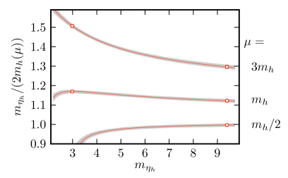
where $C_{k,PS}$ is the full perturbative series for the pseudoscalar moment and $C_{k,PS}^{(0)}$ is the leading ($\alpha_{s}^{0}$) term. So $C_{k,PS}/C_{k,PS}^{(0)}=1+c_{1}\alpha_{s}+\ldots$. For $n=4$ ($k=1$) in the pseudoscalar case we have no factor of masses in front of the series. This means that the $n=4$ moment is insensitive to the charm quark mass (it appears only in the scale for $\alpha_{s}$) and can be used to determine $\alpha_{s}$. The higher moments ($n=$ 6, 8, 10) can be used to determine $m_{c}(\mu)$ in terms of the (experimental) $\eta_{c}$ mass from equation 6. We match the lattice results at $a=0$ to the continuum perturbation theory, simultaneously fitting $n=$ 4, 6, 8 and 10 (including correlations between them and allowing for gluon condensate contributions) to extract $\alpha_{s}(\mu)$ and $M_{\eta_{c}}/m_{c}(\mu)$. The result we obtain for $m_{c}$ in the $\overline{MS}$ scheme with $n_{f}=4$ is $m_{c}(m_{c})=1.273(6)$ GeV. Note that the calculation is done with 3 flavours of sea quarks and QCD perturbation theory is used to convert to 4 flavours. A complete error budget is given in [7]. The error is dominated by the unknown higher order terms in the perturbative expansion of the moments and is estimated by including such terms with coefficients that are constrained by Bayesian priors. Information about the known $\mu$ dependence of the coefficients from the renormalisation group can be included this way. Our perturbative error is then about half the combined perturbative-$\alpha_{s}$ error in [4]. The statistical error from $\mathcal{M}_{k,latt}$ is much smaller in this case than that from $\mathcal{M}_{k,expt}$. The place in which experiment enters into the lattice calculation is in the tuning of the lattice $c$ quark mass using the experimental $\eta_{c}$ mass. For this we estimate the effect of missing electromagnetism from the lattice calculation; it is a tiny effect [13]. There is no further error from missing electromagnetism because we are comparing a lattice QCD calculation to continuum QCD perturbation theory. A further test of this approach is to calculate the vector-vector correlator and compare the moments to those extracted from experiment via $R_{c}(s)$, $\mathcal{M}_{k,expt}$, described above [17]. To extrapolate the lattice vector charmonium correlator to $a=0$ we first have to renormalise the vector current. This we do using the continuum QCD perturbation theory for the $n=4$ ($k=1$) moment. Figure 1 (right) shows the comparison of lattice QCD vector moments against $a^{2}$ with the moments determined from experiment via $R_{c}(s)$ as the black points at $a=0$. The extrapolated lattice QCD results agree well with experiment, with the lattice QCD results having approximately double the error (including a small contribution allowing for higher order QED effects which are not included in the lattice calculation but are present in experiment). This then represents an impressive 1% test of QCD and adds confidence to the determination of $m_{c}$ from the pseudoscalar moments. Using the lattice QCD vector moments to determine $m_{c}$ would give a result in agreement with that from the pseudoscalar but with a larger error. The long-time behaviour of the vector correlators simultaneously gives accurate results for the $J/\psi$ mass and leptonic width [17]. Because the HISQ action has small discretisation errors we can push to higher masses than $m_{c}$ and this was done in [7]. By extrapolating up in mass we can also determine $m_{b}$ in the $\overline{MS}$ scheme from the same method: ${m}^{(5)}_{b}({m}_{b})=4.164(23)\mathrm{GeV}$. Here the error is dominated by the extrapolation to the $b$ quark mass/$a=0$. The physical curve for the ratio of heavyonium mass to heavy quark mass is obtained on solving equation 6, and this is shown in Figure 5 (left).

Figure 5: Left: the ratio of pseudoscalar heavyonium mass to heavy quark mass in the $\overline{MS}$ scheme at scale $\mu$ as a function of heavyonium meson mass and for 3 different values of $\mu$ [7]. Notice how flat the curve is for ${m}_{h}({m}_{h})$. Right: the ratio of $c$ to $s$ quark masses determined from lattice QCD plotted against the square of the lattice spacing. Extrapolation to $a=0$ gives the physical result 11.85(16) [24].

4 Mass ratios

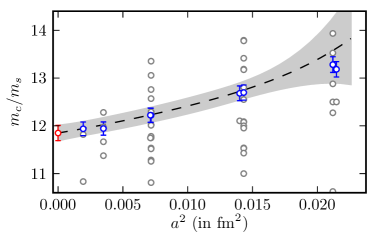
Lattice QCD enables us to determine the ratios of quark masses fully nonperturbatively. Provided that we have used the same lattice discretisation for both quarks, the $Z$ factors that connect the lattice quark mass to the $\overline{MS}$ quark mass at a given scale will cancel in the ratio. We then have, extrapolating to the continuum

$$\left(\frac{m_{q1,latt}}{m_{q2,latt}}\right)_{a=0}=\frac{m_{q1,\overline{MS}}(\mu)}{m_{q2,\overline{MS}}(\mu)}.$$ (7)

Using the HISQ action for both $c$ and $s$ quarks, fixing $am_{c}$ from $M_{\eta_{c}}$ and $am_{s}$ from $M_{K}$ (via an unphysical $s\overline{s}$ pseudoscalar particle called the $\eta_{s}$), gives the results shown in Figure 5 (right) as a function of lattice spacing. The extrapolated result, $m_{c}/m_{s}=11.85(16)$ could not be obtained with this accuracy by any other method. It enables us to convert the accurate value for $m_{c}$ discussed in the previous Section into a 1% determination of $m_{s}$. Running $m_{s}$ up from $m_{c}$ to the conventional 2 GeV gives $m_{s}(2\mathrm{GeV})$ = 92.2(1.3) MeV. In [7] we determine nonperturbatively the ratio of $m_{b}/m_{c}$, obtaining 4.51(4), and this acts as a check on the determination using moments and perturbation theory. Using mass ratios in this way we can leverage the accuracy in the heavy quark masses across the full set from $u$ to $b$ [7]. Amusingly we can use this to test the Georgi-Jarlskog expectation from GUTs that $m_{b}/m_{s}=3m_{\tau}/m_{\mu}$ [25]. For $m_{b}/m_{s}$ we have 53.4(1.1) (allowing for some statistical correlation between $m_{b}/m_{c}$ and $m_{c}/m_{s}$). This is only in marginal agreement with $3m_{\tau}/m_{\mu}$ = 50.450(5) [9]. As lattice QCD calculations become more accurate there will be more tension in simple relationships of this kind, including those between quark masses and CKM elements [26].

5 Conclusions

Both continuum and lattice QCD determinations of the $\overline{MS}$ $c$ quark mass have reached a level of accuracy around 1%. The most accurate result is ${m}_{c}^{(4)}({m}_{c})=1.273(6)$ GeV using lattice QCD [7]. This calculation used 3 flavours of sea quarks; future work is underway by both the ETM and HPQCD Collaborations to determine $m_{c}$ including $c$ quarks directly in the sea, thus removing any worries about the 3 to 4 flavour matching. To improve the accuracy on $m_{c}$ will be hard without having yet another order in QCD perturbation theory. It could be done by using a nonperturbative determination of $m_{b}/m_{c}$ and a more accurate result for $m_{b}$ from lattice QCD (using for finer lattices) because $m_{b}$ has a smaller perturbative error. It is important for phenomenologists to use these accurate values for quark masses in, for example, determination of Higgs cross-sections if they are to estimate reliably the uncertainty in the Standard Model cross-section. Currently the error on the value of $m_{c}$ being used [1, 2, 3] is inflated by a factor of 3.

ACKNOWLEDGEMENTS

I am grateful to Steve King, Peter Lepage, Paul Mackenzie, Craig McNeile and Marcus Petschlies for useful discussions. Thanks also to the organisers for a very interesting meeting.

References

- [1] S. Heinemeyer et al. [LHC Higgs Cross Section WG], arXiv:1307.1347 [hep-ph].
- [2] S. Dittmaier et al. [LHC Higgs Cross Section WG], arXiv:1201.3084 [hep-ph].
- [3] S. Dawson et al. [Snowmass 2013 Higgs WG], arXiv:1310.8361 [hep-ex].
- [4] K. G. Chetyrkin et al, Phys. Rev. D 80, 074010 (2009) [arXiv:0907.2110 [hep-ph]].
- [5] J. H. Kuhn, M. Steinhauser and C. Sturm, Nucl. Phys. B 778, 192 (2007) [arXiv:hep-ph/0702103].
- [6] I. Allison et al. [HPQCD Collaboration + Karlsruhe], Phys. Rev. D 78, 054513 (2008) [arXiv:0805.2999 [hep-lat]].
- [7] C. McNeile et al [HPQCD Collaboration], Phys. Rev. D 82, 034512 (2010) [arXiv:1004.4285 [hep-lat]].
- [8] T. DeGrand and C. E. Detar, “Lattice methods for quantum chromodynamics,” New Jersey, USA: World Scientific (2006) 345 p
- [9] J. Beringer et al. [Particle Data Group Collaboration], Phys. Rev. D 86, 010001 (2012).
- [10] R. J. Dowdall et al. [HPQCD Collaboration], Phys. Rev. D 85, 054509 (2012) [arXiv:1110.6887 [hep-lat]].
- [11] R. J. Dowdall et al [HPQCD Collaboration], Phys. Rev. D 88, 074504 (2013) [arXiv:1303.1670 [hep-lat]].
- [12] E. Follana et al. [HPQCD and UKQCD Collaborations], Phys. Rev. D 75, 054502 (2007) [arXiv:hep-lat/0610092].
- [13] C. T. H. Davies et al [HPQCD Collaboration], Phys. Rev. D 82, 114504 (2010) [arXiv:1008.4018 [hep-lat]].
- [14] S. Prelovsek, arXiv:1310.4354 [hep-lat].
- [15] R. J. Dowdall et al [HPQCD Collaboration], Phys. Rev. D 86, 094510 (2012) [arXiv:1207.5149 [hep-lat]].
- [16] J. O. Daldrop et al. [HPQCD Collaboration], Phys. Rev. Lett. 108, 102003 (2012) [arXiv:1112.2590 [hep-lat]].
- [17] G. C. Donald et al [HPQCD Collaboration], Phys. Rev. D 86, 094501 (2012) [arXiv:1208.2855 [hep-lat]].
- [18] M. E. Peskin and D. V. Schroeder, “An Introduction to quantum field theory,” Reading, USA: Addison-Wesley (1995) 842 p
- [19] R. V. Harlander and M. Steinhauser, Comput. Phys. Commun. 153, 244 (2003) [arXiv:hep-ph/0212294].
- [20] B. Dehnadi et al, JHEP 1309, 103 (2013) [arXiv:1102.2264 [hep-ph]].
- [21] K. G. Chetyrkin, J. H. Kuhn and C. Sturm, Eur. Phys. J. C 48, 107 (2006) [arXiv:hep-ph/0604234].
- [22] R. Boughezal, M. Czakon and T. Schutzmeier, Phys. Rev. D 74, 074006 (2006) [arXiv:hep-ph/0605023].
- [23] A. Maier et al, Nucl. Phys. B 824, 1 (2010) [arXiv:0907.2117 [hep-ph]].
- [24] C. T. H. Davies et al. [HPQCD Collaboration], Phys. Rev. Lett. 104, 132003 (2010) [arXiv:0910.3102 [hep-ph]].
- [25] H. Georgi and C. Jarlskog, Phys. Lett. B 86, 297 (1979).
- [26] C. McNeile, arXiv:1004.4985 [hep-lat].