Scalable iterative methods for sampling from massive Gaussian random vectors

Abstract

Sampling from Gaussian Markov random fields (GMRFs), that is multivariate Gaussian random vectors that are parameterised by the inverse of their covariance matrix, is a fundamental problem in computational statistics. In this paper, we show how we can exploit arbitrarily accurate approximations to a GMRF to speed up Krylov subspace sampling methods. We also show that these methods can be used when computing the normalising constant of a large multivariate Gaussian distribution, which is needed for both any likelihood-based inference method. The method we derive is also applicable to other structured Gaussian random vectors and, in particular, we show that when the precision matrix is a perturbation of a (block) circulant matrix, it is still possible to derive $\mathcal{O}(n\log n)$ sampling schemes.

Keywords:

Gaussian Markov random field; Lanczos algorithm; Krylov subspace; Hutchinson estimator; Markov chain Monte Carlo; Super-geometric convergence; Log-Gaussian Cox process.

1 Introduction

Sampling from large multivariate Gaussian random vectors lies at the heart of any number of tools for performing Bayesian inference. In particular, it is typically a fundamental operation in a number of popular Markov chain Monte Carlo (MCMC) methods, such as random walk Metropolis, Metropolis adjusted Langevin, and Hamiltonian Monte Carlo algorithms. When the dimension of the target distribution is large, sampling becomes a computational bottleneck and it is no longer possible, in a reasonable time frame, to use standard methods to construct samples. In this paper, we propose a new method for performing inference on models with large Gaussian components that remains feasible even when the model under consideration is massive. These methods use a controlled amount of memory and can be used to compute a sample up to arbitrary precision.

In order to obtain solutions to many high-dimensional problems within a reasonable computational budget, it is necessary to introduce additional structure to both the model and the inferential scheme. For example, in order to make models in spatial statistics computationally feasible, one is forced to make assumptions about the independence structure (Furrer et al., 2006; Kaufman et al., 2008), the conditional independence structure (Rue and Held, 2005; Lindgren et al., 2011), or enforce some sort of low dimensional structure (Higdon, 1998; Cressie and Johannesson, 2008; Banerjee et al., 2008). These assumptions, which attempt to balance computational realities with modelling flexibility, allow statisticians to fit models to relatively large spatial data sets, and to compute reasonably high-resolution spatial prediction surfaces. However, it is not uncommon to come across data sets for which these methods are not sufficient, especially when looking at space-time satellite data (Strickland et al., 2011) or three dimensional problems (Aune et al., 2011). The computational bottleneck comes in the matrix operations required to evaluate a Gaussian likelihood, compute a proposal for the Gaussian component, and for computing spatial estimates.

Given the importance of the problem, there are a large number of methods for sampling from Gaussian random vectors $\boldsymbol{x}\sim N(\boldsymbol{0},\boldsymbol{Q}^{-1})$. Typically, they revolve around computing a factorisation of the form $\boldsymbol{Q}=\boldsymbol{LL}^{T}$ and noting that $\boldsymbol{L}^{T}\boldsymbol{x}\sim N(\boldsymbol{0},\boldsymbol{I})$. The standard choice is to use the Cholesky factorisation of $\boldsymbol{Q}$, in which case $\boldsymbol{L}$ is lower triangular (Rue and Held, 2005). Another option is to chose $\boldsymbol{L}$ to be the matrix square root of $\boldsymbol{Q}$, however this will only be feasible when $\boldsymbol{Q}$ can be cheaply diagonalised. In particular, this is the case in the important situation where $\boldsymbol{Q}$ is circulant. The problem with this approach is that, as the dimension of $\boldsymbol{x}$ increases, the cost of the matrix factorisation increases sharply. In the most general case, the number of floating point operations grows as $\mathcal{O}(n^{3})$, while the memory costs grow like $\mathcal{O}(n^{2})$, where $n$ is the dimension of $\boldsymbol{x}$. On modern computers, the quadratic growth in memory will render large problems completely impossible.

In order to avoid this problem, we will focus on a class of iterative methods, known as Krylov subspace methods, initially introduced by Simpson et al. (2007) and further extended and applied by Strickland et al. (2011) and Aune et al. (2011, 2012). These methods do not require a direct factorisation (or even storage) of the matrix, but instead use modern numerical linear algebra techniques to compute $\boldsymbol{x}_{m}\approx\boldsymbol{Q}^{-1/2}\boldsymbol{z}$, where $\boldsymbol{z}$ is a vector of i.i.d. standard normal random variables and the parameter $m$ can be chosen adaptively to control the error in the approximation. These methods only require $\mathcal{O}(n)$ storage, which means that they will remain feasible for far larger problems than direct methods. Unfortunately, the number of steps that the algorithm requires to reach a prescribed error level grows polynomially in $n$, which makes them very time consuming in practice. In this article, we significantly extend the methods developed by Simpson et al. (2007) by developing tools that slow and, in some cases, completely remove this dimension-dependent cost increase. This allows us to finally construct matrix-free, dimension independent samplers for structured Gaussian random vectors.

In this paper, we will show how the structure of the Gaussian random vector can be used to make efficient, dimension-independent samplers. The paper proceeds as follows. In Section 2, we briefly review the types of structure commonly found in Gaussian random vectors, while in Section 3 we discuss efficient methods to conditionally sample from a log-Gaussian Cox process. This example will run throughout the paper and be used to demonstrate various algorithms developed in this paper. The basic Krylov sampler, as introduced in Simpson et al. (2007), is recounted in Section 4. It is shown that, even though it converges to the true sample faster than geometrically, this method does not scale well with the size of the problem. In Section 5, we develop a new method that improves the scaling of the method. In particular, though a careful re-parameterisation we can make these methods scale perfectly with dimension. We provide methods for constructing optimal, super-geometric, dimension independent, arbitrarily accurate $\mathcal{O}(n\log n)$ samplers in the case where $\boldsymbol{Q}$ is a bounded perturbation of a block circulant or block Toeplitz matrix. Guidance is also provided for building good re-parameterisations of other Gaussian random vectors, however the optimal choice is still an open research question. Although building a good sampler is an important problem, in applications it usually necessary to also be able to compute the log-density of the multivariate Gaussian random vector. The computational bottleneck here is the computation of the log-determinant of a massive matrix and in Section 6 we extend the seminal work of Hutchinson (1990) and Bai et al. (1996), as well as a some more recent work by Aune et al. (2012), to show that we can use similar re-parameterisations to construct variance-reduced Monte Carlo estimator that have dimension-independent relative error. As the estimates of the log-likelihood come from a Monte Carlo scheme, it will never be computed to high accuracy and, in Section 7, we discuss the effect of this inexactness on inference. Finally, in Section 8, we summarise the work presented in this paper and discuss some future directions.

2 Structured Gaussian random vectors

In order to motivate the methods considered in this paper, it is useful to take a closer look at the types of computationally efficient modelling structures that frequently occur. There are three common ways that $\boldsymbol{Q}$ can be structured in order to simplify computations with multivariate Gaussian random vectors. If the precision matrix $\boldsymbol{Q}$ is sparse, then this corresponds to a Markovian dependence structure between components of the random vector and such multivariate Gaussians are known as Gaussian Markov random fields (GMRFs) (Rue and Held, 2005). In this case, powerful methods from sparse linear algebra can be used to speed up computations and, when the dependence is spatial, the cost is commonly $\mathcal{O}(n^{3/2})$ (Rue, 2001). The second common structure for multivariate Gaussians occurs when the precision matrix is circulant or block circulant. These models are classically used when considering spatial models over large, regular lattices (Rue and Held, 2005; Møller et al., 1998b). As block circulant matrices can be diagonalised using fast Fourier transforms, all calculations with these multivariate Gaussians can be performed in $\mathcal{O}(n\log n)$ operations. The third common structure for multivariate Gaussians occurs when using Gaussian random fields modelled on finite dimensional stochastic processes (Cressie and Johannesson, 2008; Banerjee et al., 2008), in which case the covariance matrix is typically a sparse matrix added to a low-rank matrix. In this case, the Sherman-Morrison-Woodbury formula can be used in the computations and the cost is usually $\mathcal{O}(nr^{3})$, where $r$ is the rank of the perturbation.

The three classes of models discussed in the previous paragraph share a common characteristic: it is cheap to compute the matrix-vector product $\boldsymbol{Qv}$ for any vector $\boldsymbol{v}\in\mathbb{R}^{n}$. In fact, it is often easy to write a routine that computes the matrix-vector product without ever forming or storing the matrix $\boldsymbol{Q}$. In particular, the matrix-vector products for the three models cost, respectively, $\mathcal{O}(n)$, $\mathcal{O}(n\log n)$, and $\mathcal{O}(nr)$ operations. Furthermore, if the precision matrix of a model is, say, a circulant matrix added to a sparse matrix, it is still possible to form cheap matrix-vector products even though the model itself no longer has a special structure that classical algorithms can take advantage of.

3 Motivating example: A good MCMC sampler for log-Gaussian Cox processes

The methods described in this paper are designed to solve high-dimensional problems. While these problems arise in a number of interesting contexts, see, for example, the literature on animal breeding (Gorjanc, 2010), for simplicity we focus on problems in spatial statistics. In particular, we focus on inference for log-Gaussian Cox processes (LGCPs). This problem has all of the structure of the general type of problem that our methods will handle well, while having enough analytical structure to get results that can be used to build intuition in the more general case.

Conditional sampling from LGCPs, that is a Poisson point process for which the log intensity surface is modelled through a Gaussian random field, is a challenging problem for MCMC methods. This is a very high (actually infinite) dimensional sampling problem and, as such, it is difficult to design an MCMC scheme that efficiently explores the posterior. Given an observed point pattern $Y$, the likelihood for a LGCP can be written in hierarchical form as

$$\pi({Y}|x(\cdot)) =\exp\left(|\Omega|-\int_{\Omega}\exp(x(s))\,ds\right)\prod_{s_{i}\in Y}\exp(x(s_{i}))$$

$$x(\cdot) \sim GRF(\mu(\cdot),c(\cdot,\cdot)),$$

where $GRF(\mu(\cdot),c(\cdot,\cdot))$ is a Gaussian random field with mean function $\mu(\cdot)$ and covariance function $c(\cdot,\cdot)$. The integral in the likelihood cannot be computed analytically and, therefore, this likelihood is “doubly intractable”. Although there are a number of methods for resolving this intractability (see Girolami et al., 2013, for a survey), in this paper we will follow standard practice (Møller et al., 1998a) and approximate the likelihood. A simple way to approximate the likelihood is to discretise it over a computational lattice that covers the observation window and approximate the model with the latent Gaussian model

$$y_{ij}|x_{ij} \sim Po\left(e^{x_{ij}}\right)$$ (1a)

$$\boldsymbol{x} \sim N(\boldsymbol{0},\boldsymbol{Q}^{-1}),$$ (1b)

where $y_{ij}$ is the number of points in the $(i,j)$th cell and $\boldsymbol{x}\in\mathbb{R}^{n}$ is a stationary random field over the lattice that, for convenience, we will take to be defined on a torus with block circulant precision matrix $\boldsymbol{Q}$. It can be shown that this approximation converges as the lattice is refined (Waagepetersen, 2004).

The interesting thing about inferring LGCPs, in the context of this paper, is that the lattice structure is artificially imposed and should in practice be taken to be as fine as possible. Therefore, we are interested in developing methods that continue to work well when the dimension of the latent field is enormous. To see why this is a challenge, consider the structure of the prior distribution placed on $\boldsymbol{x}$. Due to the extremely informative nature of infinite dimensional priors and the relative lack of information present in a point pattern, it is expected that the posterior will be largely determined by the (discretised) Gaussian random field prior that has been placed on $\boldsymbol{x}$. In fact, the lack of an infinite dimensional analogue of a Lebesgue measure means that the prior distribution $\pi(\boldsymbol{x})$ will become singular as its dimension increases. Thanks to the assumption that the driving process $x(\cdot)$ is stationary on a torus, we can actually track just how singular $\boldsymbol{Q}$ becomes. It can be shown, without too much effort, that the condition number of $\boldsymbol{Q}$, that is the ratio of its largest and smallest eigenvalues grows like $\mathcal{O}(h^{-(d+2\nu)})$, where $h$ is the size of the lattice and $d$ is the dimension of the problem (hereafter taken to be equal to two), and $\nu$ is the mean square smoothness of $x(\cdot)$. This suggests that, as the lattice is refined, the problem becomes harder in floating point arithmetic (Higham, 1996) and that Gibbs samplers for sampling from $\boldsymbol{x}$ will converge slower (Roberts and Sahu, 1997; Fox and Parker, 2012) as the dimension increases. We note in passing that we can get similar growth rates from non-lattice approximations to $x(\cdot)$ (Lindgren et al., 2011) and that these can also be used to approximate log-Gaussian Cox processes (Simpson et al., 2011)

There has been an massive amount of work done on efficient MCMC methods for log-Gaussian Cox processes and the most commonly used method appears to be the preconditioned Metropolis-adjusted Langevin algorithm (MALA), which has the proposal

$$\boldsymbol{x}^{*}|\boldsymbol{x}\sim N\left(\boldsymbol{x}+\frac{\delta^{2}}{2}\boldsymbol{Q}^{-1}\nabla_{\boldsymbol{x}}\log\left(\pi(\boldsymbol{y}|\boldsymbol{x})\right),\delta^{2}\boldsymbol{Q}^{-1}\right).$$ (2)

The main advantage of this sampler is that, due to the block circulant structure of $\boldsymbol{Q}$, a proposal can be drawn using only $\mathcal{O}(n\log n)$ floating point operations and $\mathcal{O}(n)$ storage. It is, however, well accepted in the MCMC literature that when sampling from latent Gaussian models, superior samplers can be constructed by exploiting likelihood information (Rue, 2001; Christensen et al., 2006; Girolami and Calderhead, 2011). To this end, we look at the simplified manifold MALA (sMMALA) scheme of Girolami and Calderhead (2011), which has the proposal

$$\boldsymbol{x}^{*}|\boldsymbol{x}\sim N\left(\boldsymbol{x}+\frac{\delta^{2}}{2}\left(\boldsymbol{Q}+\boldsymbol{H}\right)^{-1}\nabla_{\boldsymbol{x}}\log\left(\pi(\boldsymbol{y}|\boldsymbol{x})\right),\delta^{2}(\boldsymbol{Q}+\boldsymbol{H})^{-1}\right),$$ (3)

where $\boldsymbol{H}$ is the Fisher information matrix of $\boldsymbol{y}|\boldsymbol{x}$, which is, in this case, diagonal. While this sampler performs better than the vanilla MALA (Girolami and Calderhead, 2011), the precision matrix no longer has block circulant structure and therefore requires $\mathcal{O}(n^{3})$ floating point operations and $\mathcal{O}(n^{2})$ storage to generate a proposal. Clearly this is not a feasible sampler for large lattices.

In the following sections we will show that if we carefully construct an iterative sampler, we leverage the remaining computational structure to generate a proposal from (3) using only $\mathcal{O}(n\log n)$ floating point operations and $\mathcal{O}(n)$ storage, albeit with larger suppressed constants. Therefore, it is possible to use the superior proposal scheme (3) without sacrificing the exemplary computational properties of the inferior proposal (2).

4 Krylov subspace methods for sampling from Gaussian random vectors

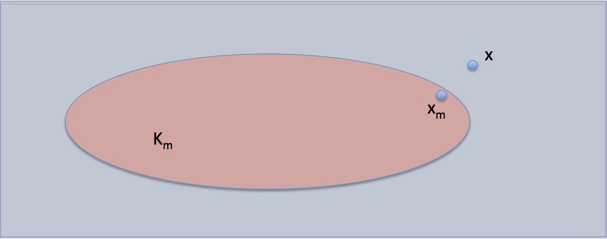
Figure 1: This figure shows a schematic representation of the Krylov sampler. Given a target sample $\boldsymbol{x}=\boldsymbol{Q}^{-1/2}\boldsymbol{z}$, the sampler constructs a sequence of subspaces $\mathcal{K}_{m}(\boldsymbol{Q},\boldsymbol{z})$ and computes a near-optimal approximation to $\boldsymbol{x}$, denoted $\boldsymbol{x}_{m}$ within this subspace. This estimate depends non-linearly on $\boldsymbol{z}$.

When it is possible to inexpensively compute the matrix-vector product $\boldsymbol{Qv}$ for arbitrary vectors $\boldsymbol{v}$, a Krylov subspace method can be constructed for sampling from $\boldsymbol{x}\sim N(\boldsymbol{0},\boldsymbol{Q}^{-1})$ (Simpson et al., 2007; Simpson, 2009; Strickland et al., 2011; Ilić et al., 2010; Aune et al., 2011). This sampler is based off the observation that, if $\boldsymbol{z}\sim N(\boldsymbol{0},\boldsymbol{I})$ is a vector of independently and identically distributed normal variables, $\boldsymbol{x}=\boldsymbol{Q}^{-1/2}\boldsymbol{z}$ is a multivariate Gaussian with precision matrix $\boldsymbol{Q}$, where $\boldsymbol{Q}^{-1/2}$ denotes the inverse of the principle square root of $\boldsymbol{Q}$. The method is then based on constructing a sequence of good approximations to $\boldsymbol{Q}^{-1/2}\boldsymbol{z}$ for a fixed realisation of $\boldsymbol{z}$. This makes our method, which is illustrated graphically in Figure 1, substantially different to the Gibbs sampler-based methods analysed by Roberts and Sahu (1997), which produce Markov chains that converge geometrically in distribution to $N(\boldsymbol{0},\boldsymbol{Q}^{-1})$. In contrast to this, we will see that due to the adaptive nature of our sampler it converges to the targeted sample faster than geometrically.

At its heart, the Krylov sampler, which is described in Algorithm 1, is a dimension reduction technique, where the sampling problem is projected onto a low-dimensional space that is sequentially constructed in such a way that it contains the main features of both the precision matrix $\boldsymbol{Q}$ and the noise vector $\boldsymbol{z}$. This idea is the basis for both the ubiquitous conjugate gradient method for solving linear systems (Saad, 1996) and the partial least squares method in applied statistics (Wold et al., 1984). In fact, it can be shown that the convergence of the Krylov sampler mirrors the convergence of the conjugate gradient method as the following theorem, which is proved in a more general form in Ilić et al. (2010), demonstrates. This bound can also be extended in a fairly straightforward manner to finite precision arithmetic (Simpson, 2009).

Theorem 1.

Let $\boldsymbol{x}_{m}$ be the sample produced in the $m$th step of the Krylov sampler and let $\boldsymbol{x}=\boldsymbol{Q}^{-1/2}\boldsymbol{z}$ be the true sample from $\boldsymbol{x}\sim N(\boldsymbol{0},\boldsymbol{Q}^{-1})$. If $\boldsymbol{r}_{m}$ is the residual at the $m$th iteration of the conjugate gradient method for solving $\boldsymbol{Qy}=\boldsymbol{z}$, then

$$\lVert\boldsymbol{x}-\boldsymbol{x}_{m}\rVert\leq\lambda_{min}^{-1/2}\lVert\boldsymbol{r}_{m}\rVert,$$ (4)

where $\lambda_{min}$ is the smallest eigenvalue of $\boldsymbol{Q}$. Furthermore, the following a priori bound holds:

$$\lVert\boldsymbol{x}-\boldsymbol{x}_{m}\rVert\leq 2\lambda_{min}^{-1/2}\sqrt{\kappa}\left(\frac{\sqrt{\kappa}-1}{\sqrt{\kappa}+1}\right)^{m}\lVert z\rVert,$$ (5)

and $\kappa=\lambda_{max}/\lambda_{min}$ is the condition number of $\boldsymbol{Q}$.

    Input: The precision matrix $\boldsymbol{Q}$ and the subspace size $m$.

Output: $\boldsymbol{x}_{m}$, an approximate sample from $N(\boldsymbol{0},\boldsymbol{Q}^{-1})$

  Sample $\boldsymbol{z}\sim N(\boldsymbol{0},\boldsymbol{I})$;

Set $\boldsymbol{v}_{1}=\boldsymbol{z}/\lVert\boldsymbol{z}\rVert$;

for $j=1:m$ do

       Set $\boldsymbol{q}=\boldsymbol{Qv}_{j}$;

       if $j\neq 1$ then

             $\boldsymbol{q}=\boldsymbol{q}-\beta_{j-1}\boldsymbol{v}_{j-1}$;

            

       end if

      $\alpha_{j}=\boldsymbol{v}_{j}^{T}\boldsymbol{q}$;

       $\boldsymbol{q}=\boldsymbol{q}-\alpha_{j}\boldsymbol{v}_{j}$;

       $\beta_{j}=\lVert\boldsymbol{q}\rVert_{2}$;

       $\boldsymbol{v}_{j+1}=\boldsymbol{q}/\beta_{j}$ ;

      

end for

Form $\boldsymbol{V}_{m}=\left[\boldsymbol{v}_{1},\boldsymbol{v}_{2},\ldots,\boldsymbol{v}_{m}\right]$ and the symmetric tridiagonal matrix $\boldsymbol{T}_{m}$ with diagonal entries $\alpha_{j}$ and sub/super-diagonal entries $\beta_{j}$;

Set $\boldsymbol{x}_{m}=\lVert\boldsymbol{z}\rVert\boldsymbol{V}_{m}\boldsymbol{T}_{m}^{-1/2}\boldsymbol{e}_{1}$, where $\boldsymbol{e}_{1}=(1,0,\ldots,0)^{T}\in\mathbb{R}^{m}$.

   

Algorithm 1 The Lanczos algorithm for approximately sampling from $N(\boldsymbol{0},\boldsymbol{Q}^{-1})$. In practice, the square root of the $m\times m$ tridiagonal matrix in the last step of the algorithm can be replaced with its rational approximation, which reduces the complexity of the final step on the sampler from $\mathcal{O}(nm+m^{3})$ to $\mathcal{O}(nm)$.

The a priori bound (5) implies that the number of iterations required to prescribed error level grows log-linearly in $\sqrt{\kappa}$. While this bound gives useful information about the qualitative convergence of the Krylov sampler, it is famously loose. Practically speaking, the valuable result in the theorem is the a posteriori bound (4), which shows that the Krylov sampler behaves in the same manner as the conjugate gradient method. Not only is this bound sufficiently tight that it can be used to evaluate the error in the Krylov sampler, but it also means that we can take the insight gathered from sixty years of practical experience with the conjugate gradient method and transfer it directly to the Krylov sampler. In particular, we know that the error will decrease “superlinearly”, that is the error will behave like $\lVert\boldsymbol{x}-\boldsymbol{x}_{m}\rVert=\text{\cal{o}}(\rho^{m})$ as $m\rightarrow\infty$ for any $\rho\in(0,1)$ (Simoncini and Szyld, 2005). This means that the Lanczos sampler will converge faster than any geometrically ergodic MCMC scheme for sampling from a multivariate Gaussian! In practice, expectations must be tempered against the challenges of floating point arithmetic, however experience suggests that the error still displays superlinear behaviour up to the point at which the error stops decreasing.

4.1 Running example: The behaviour of the Krylov sampler for sMMALA

The basic problem with the Krylov sampler, as suggested in Theorem 1, is that the size of the Krylov subspace required to capture a good approximate sample increases with the condition number of the precision matrix. In the case of our running example, as the lattice becomes denser we expect the performance of the Krylov sampler to degrade. Figure 2, which shows the decay of the upper bound (4) as the size of the lattice increases, confirms that this is indeed the case. For the largest lattice ($1024\times 1024$), a $900$ dimensional subspace is not enough to generate a good approximation.

We note that the upper bounds that are plotted are slightly misleading, in that the true error is known to be non-increasing and it is observed empirically that the point where the superlinear convergence begins (when the rate of decrease gets faster) occurs in the true error earlier than it does in the bound. However, the bound in Theorem 1 is that tightest bound the we have available and, therefore, the only available way of assessing convergence in practice.

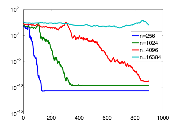
Figure 2: This figure shows the convergence of Krylov sampling applied directly to the proposal (3). The x-axis shows the subspace size, while the y-axis shows an upper bound on the error (computed with (4)).

5 Improving the efficiency of the Krylov sampler: A preconditioning approach

Although the bound in Theorem 1 suggests that the Krylov sampler may require a large number of iterations to converge, there is still hope. When solving linear systems, such as those required to compute the mean of the proposal (3), the slow convergence of the conjugate gradient method can be circumvented by a preconditioning method, in which the linear system $\boldsymbol{Qu}=\boldsymbol{z}$ is replaced with $\boldsymbol{Q}\boldsymbol{M}^{-1}\boldsymbol{u}=\boldsymbol{z}$. The choice of the precondition $\boldsymbol{M}\approx\boldsymbol{Q}$ is vital to the method and it is chosen so that it is easy to invert (Saad, 1996). For a well chosen preconditioner, the condition number of $\boldsymbol{M}^{-1}\boldsymbol{Q}$ will be close to 1, and the conjugate gradient method on the preconditioned system will then only require a few iterations for convergence.

Given that it is not possible to apply a general preconditioner built for a linear system to computing a matrix function, the preconditioning operation for the Krylov sampler is more delicate. For a linear system, the fundamental property of a practical preconditioner is that it is possible to compute $\boldsymbol{M}^{-1}\boldsymbol{b}$ quickly for any vector $\boldsymbol{b}$. The corresponding fundamental property when preconditioning the Krylov sampling turns out, unsurprisingly, to be sampling efficiently from $N(\boldsymbol{0},\boldsymbol{M}^{-1})$. This is obviously a much more difficult problem and essentially limits the types of preconditioners available to those that can be factored.

Given that we can find a matrix $\boldsymbol{M}$ such that we can sample efficiently from $N(\boldsymbol{0},\boldsymbol{M}^{-1})$, the following proposition, which can be verified using the properties of the multivariate normal distribution, outlines the method of preconditioning the Krylov sampler.

Proposition 1.

Let $\boldsymbol{Q}$ and $\boldsymbol{M}$ be symmetric positive definite matrices and let $\boldsymbol{Q}=\boldsymbol{L}\boldsymbol{L}^{T}$ and $\boldsymbol{M}=\boldsymbol{F}\boldsymbol{F}^{T}$ be given decompositions. If $\boldsymbol{u}\sim N\left(\boldsymbol{0},\left(\boldsymbol{F}^{-1}\boldsymbol{Q}\boldsymbol{F}^{-T}\right)^{-1}\right)$, then the solution to $\boldsymbol{F}^{T}\boldsymbol{x}=\boldsymbol{u}$ is a zero-mean Gaussian random vector with precision matrix $\boldsymbol{Q}$.

If the preconditioner is perfect, that is if $\boldsymbol{M}=\boldsymbol{Q}$, then $\boldsymbol{u}$ will be a vector of i.i.d. normals and the proposition collapses to the standard method for sampling from Gaussian random vectors (Rue and Held, 2005). Therefore, the dependency of $\boldsymbol{u}$ is a measure of how well $\boldsymbol{M}$ captures the essential properties of $\boldsymbol{Q}$. The key property of $\boldsymbol{u}$ is that the spectrum of $\boldsymbol{F}^{-1}\boldsymbol{Q}\boldsymbol{F}^{-T}$ will usually be much more clustered than the spectrum of $\boldsymbol{Q}$ and, therefore, the Krylov sampler will converge faster.

While Proposition 1 shows that we can replace the original sampling problem by one that may be easier to solve, we only have the vague guidance of Theorem 1, which suggests that we should make the condition number of $\boldsymbol{M}^{-1}\boldsymbol{Q}$ small, to help us choose $\boldsymbol{M}$. In the remainder of this section, we present two specific choices of $\boldsymbol{M}$ that, in turn, show the best-case and the more common place behaviour of preconditioned samplers.

5.1 Running example: Fast sampling from circulant–plus–sparse matrices

Generating a proposal from (3) requires a method to compute $\left(\boldsymbol{Q}+\boldsymbol{H}\right)^{-1}\nabla_{\boldsymbol{x}}\log\left(\pi(\boldsymbol{y}|\boldsymbol{x})\right)$ and to sample from $N\left(\boldsymbol{0},(\boldsymbol{Q}+\boldsymbol{H})^{-1}\right)$, where $\boldsymbol{Q}$ is block circulant and $\boldsymbol{H}$ is sparse. In this section, we will show that one preconditioner can be used to solve both problems. In particular, this preconditioned is optimal in the sense the the condition number of the preconditioned matrix does not depend on $h$. This means that the number of steps required for the Krylov sampler to generate a realisation of a random field up to a given accuracy depends only on the accuracy and not on the size of the mesh!

The following theorem shows that preconditioning with the prior is, in many cases, sufficient for optimal convergence.

Theorem 2.

Let $Y$ be a log-Gaussian Cox process driven by a Gaussian random field $x(s)$ defined on the flat torus $W=[0,1]^{2}$ with stationary covariance function $c(h)$. Let $\boldsymbol{y}$ be a vector of $k<\infty$ realisations the discretised LGCP on an $n_{1}\times n_{2}$ lattice and let $\boldsymbol{x}$ be the discretisation of $x(s)$ over the same lattice. If $\boldsymbol{x}_{m}$ is the approximation to a preconditioned sample $\boldsymbol{x}$ from the sMMALA proposal with preconditioner $\boldsymbol{M}_{n}=\boldsymbol{Q}_{n}+\alpha_{n}\boldsymbol{I}$, then

$$\lVert\boldsymbol{u}-\boldsymbol{u}_{m}\rVert\leq C\left(\frac{\left(\int_{W}\exp(x(s))\,ds-C_{\alpha}\right)}{m}\right)^{m},$$

where $C$ is a constant independent of $n=n_{1}n_{2}$ and $C_{\alpha}=\lim_{n\rightarrow\infty}n\alpha_{n}$. Hence if $C_{\alpha}$ is finite, then the sMMALA proposal (3) can be generated to any accuracy in $\mathcal{O}(n\log n)$ iterations.

The proof, which is given in Appendix A, relies on the prior dominating the data in the sense that $\boldsymbol{Q}_{n}^{-1}\boldsymbol{H}_{n}$ is bounded. This is commonly the case in practical spatial analysis (there are no uninformative infinite dimensional priors!), however in the rare case where there is enough data to overcome the prior, the same result holds by choosing $\boldsymbol{M}=\boldsymbol{H}$ instead of $\boldsymbol{M}=\boldsymbol{Q}$.

While Theorem 2 shows that a sampler requires $\mathcal{O}(1)$ steps to reach a fixed accuracy, the bound in the proof is very loose and does not guarantee that the number of steps required is small enough to be of practical use. In Table 1, however, we show that, for the running example, the required number of iterations is quite small. In this case $\alpha_{n}=0$ was chosen, however in practice, we can tune this parameter if required. From a practical point of view, 6 iterations of the Krylov sampler requires $24$ FFTs, in contrast to the $2$ required to solve a circulant linear system.

$m$ ($m\times m$ grid)	$16$	$32$	$64$	$128$	$256$	$512$	$1024$	$2048$	$4096$
Preconditioned	$6$	$6$	$6$	$6$	$6$	$6$	$6$	$6$	$6$
Unpreconditioned	$102$	$286$	$790$	$2166$	-	-	-	-	-

Table 1: This table, which gives the number of iterations required for the error bound (4) to be less than $10^{-8}$, demonstrates that the preconditioned sampler indeed requires $\mathcal{O}(n\log n)$ operations to reach a fixed accuracy.

5.2 Preconditioning general problems

When $\boldsymbol{Q}$ is sparse, there are several generic (or, in the nomenclature of numerical linear algebra, “algebraic”) choices of preconditioner that are available. Unlike the preconditioner considered in the previous section, algebraic preconditioners are constructed from information about the structure of the problem (sparsity pattern, block structure, etc), rather than the sort of detailed analytic knowledge used to construct the optimal preconditioner in the previous section.

The most obvious candidate for a generic preconditioner is the incomplete Cholesky decomposition (Saad, 1996) of $\boldsymbol{Q}$, which computes an approximation to the true Cholesky decomposition using a lower amount of fill in. It was shown by Wist and Rue (2006) (c.f. Hu et al., 2012) that incomplete Cholesky decompositions can be used to approximate a fixed Gaussian Markov random field. It is, therefore, expected that the incomplete Cholesky will be a successful candidate for a preconditioner in Proposition 1. A similar class of preconditioner is the factored sparse approximate inverses (Kharchenko et al., 2001), which can be constructed in parallel in a columnwise manner. It is also possible to build preconditioners based on symmetric sweeps of stationary iterative methods (Saad, 1996), which have strong connections to block Gibbs samplers in the Gaussian setting (Fox and Parker, 2012).

In Figure 3, the convergence for the preconditioned Krylov sampler is shown for several variants of the incomplete Cholesky factorisation. The test is performed on the square of the matrix constructed using the Matlab command Q = (31^2*gallery(’poisson’,30))^2, which corresponds to a second order random walk on a $30\times 30$ lattice with a modification on the boundary to ensure that the distribution is proper (see Rue and Held, 2005, for a definition). In particular, we compare incomplete Cholesky factorisations with various thresholding levels and it is clear that this simple re-parameterisation can greatly improve the performance of the Krylov sampler.

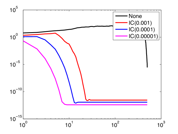
Figure 3: A comparison of incomplete Cholesky preconditioners with several thresholds. The x-axis shows the subspace size, while the y-axis shows an upper bound on the error (computed with (4)).

5.3 Connection with non-centred parameterisation

The preconditioners considered in this paper are closely linked to the concept of ‘centred’ and ‘non-centred’ parameteristations of statistical models (Papaspiliopoulos et al., 2007; Strickland et al., 2008; Yu and Meng, 2011; Filippone et al., 2013). The idea can be illustrated simply for parameter-dependent latent Gaussian models

$$\boldsymbol{y}|\boldsymbol{x},\boldsymbol{\theta} \sim\pi(\boldsymbol{y}|\boldsymbol{x},\boldsymbol{\theta})$$

$$\boldsymbol{x}|\boldsymbol{\theta} \sim N(\boldsymbol{0},\boldsymbol{Q}(\boldsymbol{\theta)}^{-1})$$

$$\theta \sim\pi(\boldsymbol{\theta}),$$

where $\pi(\cdot)$ is a generic probability density depending on its arguments. A natural way to perform inference on these models is to use a Metropolis-within-Gibbs scheme that updates all of $\boldsymbol{x}$ and all of $\boldsymbol{\theta}$ in separate blocks. The problem with this type of scheme is that $\boldsymbol{x}$ and $\boldsymbol{\theta}$ are horribly correlated in the posterior and, therefore, the Gibbs sampler will poorly explore the space. A non-centred parameterisation attempts to reduce the posterior dependence by replacing $\boldsymbol{x}$ with a new variable $\boldsymbol{u}=\boldsymbol{F}(\boldsymbol{\theta})^{T}\boldsymbol{x}$. $\boldsymbol{F}(\boldsymbol{\theta})$ is traditionally taken to be the Cholesky factor of $\boldsymbol{Q}(\boldsymbol{\theta})$, however other choices are possible.

The methods in this paper, therefore, give a new way to propose from non-centred parameterisations. It also suggests that good, computationally efficient non-centred parameterisations can be constructed from traditional preconditioners! The results in Theorem 2 can also be interpreted as a basic statement about the difference between centred and non-centred parameterisations. In fact, it corresponds well with the standard understanding that non-centred parameterisations perform well in a “low information” context, while centred parameterisations perform well in a “high information” situation (Murray and Adams, 2010).

6 Computing the log-likelihood

While sampling from a large Gaussian random variable is all that is required for many MCMC proposals, if the latent field $\boldsymbol{x}$ in (1) depends on some unknown parameters, computing the acceptance ratio will require the computation of a ratio of determinants of $\boldsymbol{Q}(\boldsymbol{\theta})$, where $\boldsymbol{\theta}$ are now some unknown parameters. Unlike when using Cholesky decompositions to sample from Gaussian random vectors, the Krylov methods considered in this paper do not automatically construct an approximation to the log-determinant. While it is difficult to construct efficient, arbitrarily accurate approximations to the log-determinant, there is a straightforward unbiased Monte Carlo estimate. Bai et al. (1996) used a variant of the Hutchinson estimator (Hutchinson, 1990) to construct the estimate

$$\log(\det(Q))=\mathbb{E}_{\mathcal{V}}(\mathcal{V}^{T}\log(\boldsymbol{Q})\mathcal{V})\approx N^{-1}\sum_{i=1}^{N}\boldsymbol{v}_{i}^{T}\log(\boldsymbol{Q})\boldsymbol{v}_{i},$$

where the components of $\boldsymbol{v}_{i}$ are i.i.d. with values equal to $\pm 1$ with equal probability, that is, $\mathcal{V}$ is a vector with i.i.d. Rademacher components.

Hutchinson (1990) showed that the above estimator is unbiased and the choice of random vectors gives the minimum variance estimator amongst all centred, uncorrelated random vectors. However, the variance, which is $\lVert\log(\boldsymbol{Q})\rVert_{F}^{2}-\operatorname{tr}(\log(\boldsymbol{Q}))^{2}$, can still be unacceptably large in practical situations. We suggest a combination of two novel techniques to help reduce the variance to a more manageable level. The first method to reduce the variance was introduced by Aune et al. (2012) using a combination of ad hoc reasoning and numerical experimentation. In the following paragraphs, we will re-derive this method rigorously and show that the resulting variance reduction is due to the structure of $\boldsymbol{Q}$. We will use the insight built in this derivation to show how to build preconditioners that maintain the efficiency of the method of Aune et al. (2012) as the dimension of the problem increases.

6.1 Understanding the coloured Hutchinson estimator of Aune et al. (2012)

In order to ease notation, we will use the notation $\boldsymbol{B}=\log(\boldsymbol{Q})$ in the remainder of this section and, for the sake of simplicity, we will assume for the rest of this section that $\boldsymbol{Q}$ is sparse. For a realisation $\boldsymbol{v}$ of the vector valued random variable $V$, then, by the symmetry of $\boldsymbol{B}$,

$$\boldsymbol{v}^{T}\boldsymbol{Bv}=\operatorname{tr}(\boldsymbol{B})+2\sum_{i<k}v_{i}v_{j}B_{ij},$$

where $v_{i}$ is the $i$th component of $\boldsymbol{v}$ and $B_{ij}$ is similarly defined. It is clear that the off-diagonal elements of $\boldsymbol{B}$ are the source of the Monte Carlo error. The off diagonal elements of $\boldsymbol{B}$ are not arbitrary. Benzi and Razouk (2007) proved that the entries decay exponentially in the graph distance $d(i,j)$. Let the eigenvalues of $\boldsymbol{Q}$ be contained in the interval $[\lambda_{\min},\lambda_{\max}]$. Then a combination of Theorem 3.4 and the discussion in Section 3.7 of Benzi and Razouk (2007) show that, for any $1<2R<2R^{*}$,

$$B_{ij}\leq\frac{2}{1-1/(2R)}\max_{t=\pm(R+1/(4R))}\left|\log\left(\frac{1}{2}\left((\lambda_{\max}-\lambda_{\min})t+\lambda_{\max}+\lambda_{\min}\right)\right)\right|(2R)^{-d(i,j)},$$ (6)

where $R^{*}$ is the smallest value larger than one for which the bound is undefined.

Given that the off-diagonal elements of $\boldsymbol{B}$ pollute the Hutchinson estimator, and given that the off diagonal elements of $\boldsymbol{B}$ decay geometrically, it makes sense to decompose $\mathcal{V}$ in order to avoid the large elements. Formally, the strategy of Aune et al. (2012) to reduce the variance of the Hutchinson estimator is to decompose the random vectors as $\mathcal{V}=\bigoplus_{\mathfrak{c}\in\mathcal{C}}\mathcal{V}^{\mathfrak{c}}$, where $\mathcal{C}$ is a non-overlapping partition of $\{1,\ldots,n\}$ and $\mathcal{V}^{\mathfrak{c}}$ is a random vector in which the $i$th component has an independent Rademacher distribution if $i\in\mathfrak{c}$ and is zero otherwise. The coloured Hutchinson estimator is then

$$\log(\det(\boldsymbol{Q}))=\mathbb{E}(\mathcal{V}^{T}\log(\boldsymbol{Q})\mathcal{V})=\sum_{\mathfrak{c}\in\mathcal{C}}\mathbb{E}((\mathcal{V}^{\mathfrak{c}})^{T}\log(\boldsymbol{Q})\mathcal{V}^{\mathfrak{c}})$$

and its variance is given by

$$\operatorname{Var}(\mathcal{V}^{T}\log(\boldsymbol{Q})\mathcal{V}) =\sum_{\mathfrak{c}\in\mathcal{C}}\operatorname{Var}((\mathcal{V}^{\mathfrak{c}})^{T}\log(\boldsymbol{Q})\mathcal{V}^{\mathfrak{c}})$$

$$=\sum_{i\neq j\in\mathfrak{c}\times\mathfrak{c}}B_{ij}^{2}$$

$$\leq C^{2}\sum_{i\neq j\in\mathfrak{c}\times\mathfrak{c}}(2R)^{-2d(i,j)},$$ (7)

where $C$ is the constant (in $d(i,j)$) term in (6). Following a suggestion by Tang and Saad (2012), Aune et al. (2012) constructed the partition $\mathcal{C}$ by colouring the graph corresponding to the sparsity structure of $\boldsymbol{Q}^{p}$ for some small number $p$. This ensures that, for all $i,j\in\mathfrak{c}$, $d(i,j)>p$ and shows that the variance of the coloured Hutchinson estimator will be reduced.

The variance reduction and unbiasedness of the coloured Hutchinson estimator is demonstrated in Figure 4.

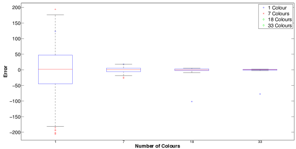
Figure 4: This figure shows that a box plot of $\boldsymbol{v}^{T}\log(\boldsymbol{Q})\boldsymbol{v}$ for the coloured Hutchinson estimator of the matrix considered in Section 5.2. From left to right, there boxes correspond to the uncoloured Hutchinson estimator, the 1-coloured, 2-coloured, and 3-coloured Hutchinson estimators. It is clear that these are unbiased.

6.2 The role of preconditioning

Unfortunately, the bound (6) shows that the there is strong mesh dependence. Careful analysis shows that $R^{*}=\frac{1}{2}+\mathcal{O}(\kappa^{-1/2})$, which implies that the distant (in the graph metric) values of $B_{ij}$ become more and more important as the dimension of the problem increases. Logically, this is not particularly surprising. If you consider the infill situation that occurs when modelling log-Gaussian Cox processes (the window is fixed, the size of the grid cell decreases), then it is clear that the graph distance does not mirror the physical distance as the dimension of the system increases. Fortunately, there is a remedy for this.

Following the theme of the previous section, we note that determinants can also be preconditioned. In particular,

$$\log\det(\boldsymbol{Q})=\log\det\left(\boldsymbol{F}^{-1}\boldsymbol{Q}\boldsymbol{F}^{-T}\right)-2\log\det(\boldsymbol{F}).$$

If the log determinant of $\boldsymbol{F}$ is known by construction, then one only needs to approximate $\log\det\left(\boldsymbol{F}^{-1}\boldsymbol{Q}\boldsymbol{F}^{-T}\right)$, which should be significantly better behaved than the original problem. In fact, if $\boldsymbol{M}=\boldsymbol{FF}^{T}$ is an optimal preconditioner, than the bound in equation (6) suggests that the $\mathcal{R}^{*}$ is independent of $n$. This suggests that a good preconditioner will give a similar variance reduction for each colouring regardless of the dimension of the problem.

In the case of the log-Gaussian Cox process, the proof of Theorem 2 shows that $\boldsymbol{Q}_{n}^{-1}\boldsymbol{H}_{n}$ converges to a trace class operator as $n\rightarrow\infty$ and, therefore, it follows from the theory of Fredholm determinants (Bornemann, 2009) that $\log\det\left(\boldsymbol{F}_{n}^{-1}\boldsymbol{Q}_{n}\boldsymbol{F}_{n}^{-T}\right)$ stays bounded. This is important as the computation of the log-acceptance ratio requires the difference of log-determinants and it is computationally unwise to compute the difference of large floating point numbers!

7 Whither exactness? Balancing the inexactness of Krylov methods with the inexactness of MCMC

In this paper, we showed that the Krylov methods can be used to compute samples and likelihoods of Gaussian models in a way that can be independent of the dimension of the underlying problem. These methods are necessary in order to perform inference on massive statistical models. In order to make inference possible on these models, we have sacrificed a degree of exactness and it is reasonable to ask what effect this has on inference methods.

Samples computed using Krylov sampling are not Gaussian. The algorithm works by targeting a fixed sample from a multivariate Gaussian and approximating it within a low-dimensional subspace that is constructed using information from the target sample. Therefore, rather than computing the linear filter $\boldsymbol{Q}^{-1/2}\boldsymbol{z}$, we are instead computing a complicated non-linear function of the Gaussian random vector $\boldsymbol{z}$. The question is then: does this matter? From a pragmatic point of view, we argue that it doesn’t. There are essentially two components to our argument. The first is an appeal to practicality, where we must admit that by the time that these algorithms are of any use at all, the problems that are being solved are sufficiently difficult that some sacrifices are needed. There is also strong evidence that being slightly wrong is not a problem in practical MCMC schemes as the incorrect chain will often follow the “correct” chain for a long period of time (Nicholls et al., 2012). The second argument is an appeal to reality. This cardinal rule of numerical computing is that you will never calculate the exact thing that you wish to. Floating point artefacts pollute even the simplest numerical calculations and in the situations that we have considered in this paper, where we are approximating an infinite dimensional random variable by a high dimensional one, these calculations are anything but simple. Even an “exact” sample computed using a Cholesky factorisation, which is the current gold standard for sampling from large problem, will, in reality, be non-Gaussian due to to the complicated effect of rounding error. For the sorts of problems considered in this paper, methods based on the Cholesky factorisation will not be exact within floating point tolerance.

A different, but related, difficulty comes from the inexact calculation of the log-determinant. While this is unbiased, it will lead to a biased estimator of the acceptance ratio, which is a ratio of determinants. Girolami et al. (2013) showed that it is possible to account for this extra randomness and construct an exact pseudo-marginal MCMC scheme. However, in the interest of simplicity, we have opted to work with an inexact chain. Once again, the analysis of Nicholls et al. (2012) strongly suggests that inexact MCMC schemes that simply use the estimate directly (or those that adjust for the variance in the estimator) will lead to methods that are, for all intents and purposes, exact. They argue that the inexact chain will be coupled with the true chain for, on average, an amount of time proportional to the inverse variance of the estimator. This means that if the estimator is sufficiently precise, the error cause by the inexactness of the chain will most likely be swamped by the Monte Carlo error.

The fundamental question, then, becomes not one of accuracy and asymptotic exactness, but rather one of finite sample behaviour. Ideally, we would like to have a detailed theory that links the accuracy of each step of the MCMC scheme with the finite sample error. Outside of statistics, this is analogous to the analysis of Dembo et al. (1982) for Newton’s method for solving systems non-linear equations, in which it was shown that the quadratic convergence of Newton’s method can be maintained even when the correction term in computed inexactly. To the best of our knowledge, the general version of this problem has not been solved, however the recent work of Ketelsen et al. (2013), in which detailed work was done to balance error and cost for a class of inverse problems.

8 Conclusion

The methods presented in this paper open up the possibility of general, dimension independent inference methods. There are a number of further steps required to make this dream a reality. First and foremost, a great deal of effort must be put into constructing optimal or almost optimal preconditioners that can be factorised. In this paper we showed that this is possible, however we limited ourselves to (block) circulant problems. While the extension to Toeplitz matrices is straightforward, block Toeplitz matrices pose a significant challenge. In this case, optimal preconditioners have a banded block Toeplitz form (Serra, 1994). It is possible to sample from the optimal in $\mathcal{O}((n\log n)$ operations by combining multigrid methods with a rational approximation to the square root (Hale et al., 2008) and to compute determinants in $\mathcal{O}(n^{3/2}\log(n))$ operations (Bini and Pan, 1988). These preconditioners are, therefore, much more expensive than in the circulant case.

This highlights a fundamental challenge for this methodology. At the current time, the gold-standard method for constructing mesh-independent preconditioners for general spatial problems is to use some variant of multigrid, however this procedure cannot be used in our context as it is not possible to sample from a Gaussian vector with a precision operator given by the multigrid operation. A more promising option may be symmetric sweep Schwartz iterations, which have a strong connection with overlapping block Gibbs samplers for sampling from large Gaussian random vectors. Another challenge is to construct preconditioners that have mesh-independent decay properties. This is needed to ensure that the variance of the preconditioned determinant calculation can be bounded independent of the dimension of the problem. It is also important to design and study “algebraic” preconditioners (such as incomplete Cholesky factorisations) that can be applied to general problems without using some underlying analytical structure of the problem.

The second challenge that must be met for these methods to implement these methods in fast, efficient ways. Aune et al. (2011) has considered the use of GPUs for sampling from large Gaussian random vectors, while Rue (2001) has used shared memory parallelisation to speed up the INLA software (Rue et al., 2009). Paciorek et al. (2013) use MPI to distribute the dense linear algebra operations required for inference with general, unstructured covariance matrices. The methods considered in that paper are limited to small problems, however this type of parallelism is certainly useful for distributing Krylov methods.

The final challenge is in the design of MCMC samplers that mirror the dimension independence of the Krylov sampler. There has been some work done in generalising basic samplers like preconditioned Crank-Nicolson (Cotter et al., 2012), preconditioned MALA (Beskos et al., 2008) and Hamiltonian Monte Carlo (Beskos et al., 2011) to this case, but this technology has yet to be employed on methods that try to track the local second order properties of the posterior. With these three steps in place, we believe that the methods presented in this paper will have a great impact on inference schemes for massive problems.

Acknowledgements:

The authors would like to thank Erlend Aune, Colin Fox, Al Parker and Håvard Rue for their feedback and encouragement.

Appendix A Proof of Theorem 2

Without loss of generality, we can take $k=1$.

Noting that $\mathbf{M}_{n}^{-1}(\boldsymbol{Q}_{n}+\boldsymbol{H}_{n})=(\boldsymbol{Q}_{n}+\alpha_{n}\boldsymbol{I}_{n})^{-1}(\boldsymbol{H}_{n}-\alpha_{n}\boldsymbol{I}_{n})$, if follows that if, $\operatorname{tr}(\boldsymbol{Q}_{n}^{-1}\boldsymbol{H}_{n})$ is bounded for all $n$, the result follows from Theorem 1 and the results of Axelsson and Karátson (2009). The boundedness of the trace can be shown as follows.

$$\operatorname{tr}\left((\boldsymbol{Q}_{n}+\alpha_{n}\boldsymbol{I}_{n})^{-1}(\boldsymbol{H}_{n}-\alpha_{n}\boldsymbol{I}_{n})\right) =\left[(\boldsymbol{Q}_{n}+\alpha_{n}\boldsymbol{I}_{n})^{-1}\right]_{1,1}\sum_{i=1}^{n}(h^{2}e^{x_{i}}-\alpha_{n})$$

$$=\left[(\boldsymbol{Q}_{n}+\alpha_{n}\boldsymbol{I}_{n})^{-1}\right]_{1,1}\left(\int_{W}\exp(x(s))\,ds+O(h^{2})-n\alpha_{n}\right)$$

$$\rightarrow C\left(\int_{W}\exp(x(s))\,ds-C_{\alpha}\right)<\infty\,\text{a.s.}$$

References

- Aune et al. (2011) Erlend Aune, Jo Eidsvik, and Yvo Pokem. Iterative numerical methods for sampling from high dimensional gaussian distributions. Technical Report 4/2011, NTNU, 2011.
- Aune et al. (2012) Erlend Aune, Daniel Simpson, and Jo Eidsvik. Parameter estimation in high dimensional gaussian distributions. Technical Report Statistics 5/2012, NTNU, 2012.
- Axelsson and Karátson (2009) O. Axelsson and J. Karátson. Equivalent operator preconditioning for elliptic problems. Numerical Algorithms, 50(3):297–380, 2009.
- Bai et al. (1996) Z. Bai, G. Fahey, and G. Golub. Some large-scale matrix computation problems. Journal of Computational and Applied Mathematics, 74(1):71–89, 1996.
- Banerjee et al. (2008) S. Banerjee, A. E. Gelfand, A. O. Finley, and H. Sang. Gaussian predictive process models for large spatial datasets. Journal of the Royal Statistical Society, Series B, 70(4):825–848, 2008.
- Benzi and Razouk (2007) Michele Benzi and Nader Razouk. Decay bounds and o (n) algorithms for approximating functions of sparse matrices. Electronic Transactions on Numerical Analysis, 28:16–39, 2007.
- Beskos et al. (2008) Alexandros Beskos, Gareth Roberts, Andrew Stuart, and Jochen Voss. Mcmc methods for diffusion bridges. Stochastics and Dynamics, 8(03):319–350, 2008.
- Beskos et al. (2011) Alexandros Beskos, FJ Pinski, JM Sanz-Serna, and AM Stuart. Hybrid monte carlo on hilbert spaces. Stochastic Processes and their Applications, 121(10):2201–2230, 2011.
- Bini and Pan (1988) D Bini and V Pan. Efficient algorithms for the evaluation of the eigenvalues of (block) banded toeplitz matrices. Mathematics of computation, 50(182):431–448, 1988.
- Bornemann (2009) F. Bornemann. On the numerical evaluation of fredholm determinants. Mathematics of Computation, 79(270):871, 2009.
- Christensen et al. (2006) O. F. Christensen, G. O. Roberts, and M. Sköld. Robust Markov chain Monte Carlo methods for spatial generalised linear mixed models. Journal of Computational and Graphical Statistics, 15(1):1–17, 2006.
- Cotter et al. (2012) Simon Cotter, Gareth Roberts, Andrew Stuart, and David White. Mcmc methods for functions: modifying old algorithms to make them faster. arXiv preprint arXiv:1202.0709, 2012.
- Cressie and Johannesson (2008) N. A. C. Cressie and G. Johannesson. Fixed rank kriging for very large spatial data sets. Journal of the Royal Statistical Society, Series B, 70(1):209–226, 2008.
- Dembo et al. (1982) Ron S Dembo, Stanley C Eisenstat, and Trond Steihaug. Inexact newton methods. SIAM Journal on Numerical analysis, 19(2):400–408, 1982.
- Filippone et al. (2013) Maurizio Filippone, Mingjun Zhong, and Mark Girolami. A comparative evaluation of stochastic-based inference methods for Gaussian process models. Machine Learning, 2013. URL http://dx.doi.org/10.1007/s10994-013-5388-x.
- Fox and Parker (2012) Colin Fox and Albert Parker. Convergence in variance of first-order and second-order Chebyshev accelerated Gibbs samplers. Submitted, 2012.
- Furrer et al. (2006) R. Furrer, M. G. Genton, and D. Nychka. Covariance tapering for interpolation of large spatial datasets. J. Comput. Graph. Statist., 15(3):502–523, 2006.
- Girolami and Calderhead (2011) M. Girolami and B. Calderhead. Riemann manifold Langevin and Hamiltonian monte carlo methods. Journal of the Royal Statistical Society: Series B (Statistical Methodology), 73(2):123–214, 2011.
- Girolami et al. (2013) Mark Girolami, Anne-Marie Lyne, Heiko Strathmann, Daniel Simpson, and Yves Atchade. Playing Russian roulette with intractable likelihoods. In preparation, 2013.
- Gorjanc (2010) Gregor Gorjanc. Graphical model representation of pedigree based mixed model. In 2010 32nd International Conference on Information Technology Interfaces (ITI), pages 545–550. IEEE, 2010.
- Hale et al. (2008) Nicholas Hale, Nicholas J Higham, and Lloyd N Trefethen. Computing a^,log(a), and related matrix functions by contour integrals. SIAM Journal on Numerical Analysis, 46(5):2505–2523, 2008.
- Higdon (1998) D. Higdon. A process-convolution approach to modelling temperatures in the North Atlantic Ocean. Environmental and Ecological Statistics, 5(2):173–190, 1998.
- Higham (1996) Nicholas J Higham. Accuracy and Stability of Numerical Analysis. Number 48. Siam, 1996.
- Hu et al. (2012) Xiangping Hu, Daniel Simpson, and Håvard Rue. Specifying gaussian markov random fields with incomplete orthogonal factorization using givens rotations. Technical Report Statistics xx/2012, NTNU, 2012.
- Hutchinson (1990) M. F. Hutchinson. A stochastic estimator of the trace of the influence matrix for laplacian smoothing splines. J. Commun. Statist. Simula., 19(2):433–450, 1990.
- Ilić et al. (2010) M. Ilić, I. W. Turner, and Daniel Simpson. A restarted Lanczos approximation to functions of a symmetric matrix. IMA Journal on Numerical Analysis, 30(4):1044–1061, 2010.
- Kaufman et al. (2008) C.G. Kaufman, M.J. Schervish, and D.W. Nychka. Covariance tapering for likelihood-based estimation in large spatial data sets. Journal of the American Statistical Association, 103(484):1545–1555, 2008.
- Ketelsen et al. (2013) C Ketelsen, R Scheichl, and AL Teckentrup. A hierarchical multilevel markov chain monte carlo algorithm with applications to uncertainty quantification in subsurface flow. arXiv preprint arXiv:1303.7343, 2013.
- Kharchenko et al. (2001) SA Kharchenko, L Yu Kolotilina, AA Nikishin, and A Yu Yeremin. A robust ainv-type method for constructing sparse approximate inverse preconditioners in factored form. Numerical linear algebra with applications, 8(3):165–179, 2001.
- Lindgren et al. (2011) F. Lindgren, H. Rue, and J. Lindström. An explicit link between Gaussian fields and Gaussian Markov random fields: The stochastic partial differential equation approach (with discussion). Journal of the Royal Statistical Society. Series B. Statistical Methodology, 73(4):423–498, September 2011.
- Møller et al. (1998a) J. Møller, A. R. Syversveen, and R. P. Waagepetersen. Log Gaussian Cox processes. Scandinavian Journal of Statistics, 25:451–482, 1998a.
- Møller et al. (1998b) J. Møller, A. R. Syversveen, and R. P. Waagepetersen. Log Gaussian Cox processes. Scandinavian Journal of Statistics, 25:451–482, 1998b.
- Murray and Adams (2010) Iain Murray and Ryan Prescott Adams. Slice sampling covariance hyperparameters of latent Gaussian models. In J. Lafferty, C. K. I. Williams, R. Zemel, J. Shawe-Taylor, and A. Culotta, editors, Advances in Neural Information Processing Systems 23, pages 1723–1731. 2010.
- Nicholls et al. (2012) Geoff K Nicholls, Colin Fox, and Alexis Muir Watt. Coupled MCMC with a randomized acceptance probability. arXiv preprint arXiv:1205.6857, 2012.
- Paciorek et al. (2013) Christopher J. Paciorek, Benjamin Lipshitz, Wei Zhuo, Prabhat, Cari G. Kaufman, and Rollin C. Thomas. Parallelizing gaussian process calculations in R. arXiv preprint arXiv:1305.4886, 2013.
- Papaspiliopoulos et al. (2007) Omiros Papaspiliopoulos, Gareth O Roberts, and Martin Sköld. A general framework for the parametrization of hierarchical models. Statistical Science, pages 59–73, 2007.
- Roberts and Sahu (1997) G. O. Roberts and S. K. Sahu. Updating schemes, correlation structure, blocking and parameterization for the Gibbs sampler. Journal of the Royal Statistical Society, Series B, 59(2):291–317, 1997.
- Rue (2001) H. Rue. Fast sampling of Gaussian Markov random fields. Journal of the Royal Statistical Society, Series B, 63(2):325–338, 2001.
- Rue and Held (2005) H. Rue and L. Held. Gaussian Markov Random Fields: Theory and Applications, volume 104 of Monographs on Statistics and Applied Probability. Chapman & Hall, London, 2005.
- Rue et al. (2009) H. Rue, S. Martino, and N. Chopin. Approximate Bayesian inference for latent Gaussian models using integrated nested Laplace approximations (with discussion). Journal of the Royal Statistical Society, Series B, 71(2):319–392, 2009.
- Saad (1996) Y. Saad. Iterative Methods for Sparse Linear Systems. The PWS Series in Computational Science. PWS Publishing Company, 1996.
- Serra (1994) Stefano Serra. Preconditioning strategies for asymptotically ill-conditioned block toeplitz systems. BIT Numerical Mathematics, 34(4):579–594, 1994.
- Simoncini and Szyld (2005) Valeria Simoncini and Daniel B Szyld. On the occurrence of superlinear convergence of exact and inexact krylov subspace methods. SIAM review, 47(2):247–272, 2005.
- Simpson (2009) Daniel Simpson. Krylov subspace methods for approximating functions of symmetric positive definite matrices with applications to applied statistics and anomalous diffusion. PhD thesis, Queensland University of Technology, 2009.
- Simpson et al. (2011) Daniel Simpson, Janine Illian, Finn Lindgren, Sigrunn Sørbye, and Håvard Rue. Computationally efficient inference for log-gaussian cox processes. Submitted, 2011.
- Simpson et al. (2007) D.P. Simpson, I.W. Turner, and A.N. Pettitt. Fast sampling from a Gaussian Markov random field using Krylov subspace approaches. Technical report, Queensland University of Technology, 2007.
- Strickland et al. (2011) C. M. Strickland, D. P. Simpson, I. W. Turner, r. Denham, and K. L. Mengersen. Fast bayesian analysis of spatial dynamic factor models for multitemporal remotely sensed imagery. Journal of the Royal Statistical Society : Series C, 60(1):109–124, January 2011.
- Strickland et al. (2008) Chris M Strickland, Gael M Martin, and Catherine S Forbes. Parameterisation and efficient mcmc estimation of non-gaussian state space models. Computational Statistics & Data Analysis, 52(6):2911–2930, 2008.
- Tang and Saad (2012) Jok M Tang and Yousef Saad. A probing method for computing the diagonal of a matrix inverse. Numerical Linear Algebra with Applications, 19(3):485–501, 2012.
- Waagepetersen (2004) R. Waagepetersen. Convergence of posteriors for discretized log Gaussian Cox processes. Statistics & Probability Letters, 66(3):229–235, 2004.
- Wist and Rue (2006) H. T. Wist and H. Rue. Specifying a Gaussian Markov random field by a sparse Cholesky triangle. Communications in Statistics: Simulation and Computation, 35(1):161–176, 2006.
- Wold et al. (1984) S. Wold, A. Ruhe, H. Wold, and WJ Dunn III. The collinearity problem in linear regression. the partial least squares (pls) approach to generalized inverses. SIAM Journal on Scientific and Statistical Computing, 5(3):735–743, 1984.
- Yu and Meng (2011) Yaming Yu and Xiao-Li Meng. To center or not to center: That is not the question—an ancillarity–sufficiency interweaving strategy (asis) for boosting mcmc efficiency. Journal of Computational and Graphical Statistics, 20(3):531–570, 2011.