Precise predictions for $A_{H}q_{-}$ associated production in the littlest Higgs model with $T$ parity at the LHC

Abstract

In the framework of the littlest Higgs model with $T$ parity, we present complete calculations for the $A_{H}q_{-}$ $(q_{-}=u_{-},\bar{u}_{-},d_{-},\bar{d}_{-},c_{-},\bar{c}_{-},s_{-},\bar{s}_{-})$ associated production up to the QCD next-to-leading order (NLO) at the CERN Large Hadron Collider with subsequent pure weak decay of $T$-odd mirror quark. We apply the PROSPINO scheme to avoid the double counting problem and to keep the convergence of the perturbative QCD description. The theoretical correlations between the integrated cross section and the factorization and renormalization scale, the global symmetry-breaking scale and the Yukawa coupling parameter are studied separately. We also provide the kinematic distributions of the final decay products. Our numerical results show that the NLO QCD correction reduces the scale uncertainty and enhances the leading-order integrated cross section remarkably, with the $K$ factor varying in the range of $1.41\sim 1.68$ ($1.58\sim 1.89$) as the increment of the global symmetry-breaking scale $f$ from $500~{}{\rm GeV}$ to $1.5~{}{\rm TeV}$ ($1.1~{}{\rm TeV}$) at the $\sqrt{s}=14~{}{\rm TeV}$ ($8~{}{\rm TeV}$) LHC. We find that it is possible to select the signal events of the $A_{H}q_{-}$ production from its background by putting proper cuts on the final leading jet and missing energy.

PACS: 12.38.Bx, 12.60.Cn, 14.70.Pw

I. Introduction

The standard model (SM) [1, 2] provides an excellent description of high-energy phenomena at the energy scale up to $10^{2}~{}{\rm GeV}$. However, several theoretical problems [3] that the SM encounters still make us confused, and drive physicists to consider new physics beyond the SM. Many extensions of the SM are proposed to deal with these problems, such as supersymmetric models [4], extra dimensions models [5], little Higgs models [6], grand unified theories [7], and so on. Among them, the little Higgs models deserve much attention due to their elegant solution to the hierarchy problem, and are proposed as one kind of electroweak symmetry-breaking (EWSB) model without fine tuning, in which the Higgs boson is naturally light as a result of nonlinearly realized symmetry [8, 9]. The simplest version of the little Higgs models is the littlest Higgs model (LH) [10], which is based on an $SU(5)/SO(5)$ nonlinear $\sigma$ model. In the LH, a set of new heavy gauge bosons ($A_{H},Z_{H},W_{H}^{\pm}$) and a vectorlike quark ($T$) are introduced to cancel the quadratic divergence of the Higgs boson mass contributed by the SM gauge boson loops and the top quark loop, respectively. However, the present precision electroweak constraints [11, 12, 13] require the LH to be characterized by a large value of the global symmetry-breaking scale $f$, so the fine tuning between the cutoff scale and the electroweak scale is again needed. Fortunately, this problem can be solved by introducing a discrete symmetry, the $T$ parity, to the LH [14, 15].

In the littlest Higgs model with $T$ parity (LHT), all the SM particles are $T$-even and all the new heavy particles except $T_{+}$ are $T$ odd. Then the SM gauge bosons cannot mix with the new heavy gauge bosons, and the global symmetry-breaking scale $f$ can be lower than $1~{}{\rm TeV}$ [16]. Recently, from the analyses of Higgs data from the ATLAS and CMS Collaborations combined with other experimental results, we get the constraint on the scale $f$ in the LHT as $f>694~{}{\rm GeV}$ given in Ref.[12] and $f>665~{}{\rm GeV}$ provided in Ref.[13]. In the LHT, the decay channels $W_{H}^{\mp}\to l^{\mp}\stackrel{{\scriptstyle(-)}}{{\nu}}$ and $Z_{H}\to l^{+}l^{-}$ are forbidden, and the probable decay modes of these heavy gauge bosons should be $T$-parity conserving. What’s more, the LHT offers a candidate for dark matter, called the heavy photon $A_{H}$, which cannot decay into other particles. As more and more attention is paid to dark matter [17], the precision investigation for $A_{H}$ production will be meaningful and necessary.

In this paper, we focus on the $A_{H}q_{-}$ production up to the QCD NLO, where $q_{-}$ represents the $T$-odd mirror quark of the first two generations. A brief review of the related LHT theory can be found in Sec.II. In Sec.III, we provide our calculation strategy. The numerical results and discussions are presented in Sec.IV. Finally a short summary is given.

II. Related LHT theory

In this section, we will briefly review the LHT theory related to our calculations. For more details, one can refer to Refs.[18, 19, 20].

The LH is based on a nonlinear $\sigma$ model describing the spontaneous breaking of an $SU(5)$ global symmetry down to its $SO(5)$ subgroup at an energy scale $f\sim 1~{}{\rm TeV}$. This symmetry breaking originates from the vacuum expectation value (VEV) of an $SU(5)$ symmetric tensor field $\Sigma$, given by

$$\Sigma_{0}=\langle\Sigma\rangle=\left(\begin{array}[]{ccccc}&&1_{2\times 2}\\ &1&\\ 1_{2\times 2}&&\end{array}\right).$$ (2.4)

Then the nonlinear $\sigma$ model tensor field $\Sigma$ can be written as

$$\Sigma=e^{i\Pi/f}\Sigma_{0}e^{i\Pi^{T}/f}=e^{2i\Pi/f}\Sigma_{0},$$ (2.5)

where $\Pi(x)$ is the “pion” matrix containing the 14 Nambu-Goldstone degrees of freedom from the $SU(5)/SO(5)$ breaking. An $[SU(2)\times U(1)]_{1}\times[SU(2)\times U(1)]_{2}$ subgroup of the $SU(5)$ global symmetry is gauged in the LH, and the gauge fields $W_{i\mu}^{a}$ and $B_{i\mu}$ $(a=1,2,3,~{}i=1,2)$ are introduced. To implement $T$ parity in the LHT, we make the following $T$ parity assignment:

$$W_{1\mu}^{a}\longleftrightarrow W_{2\mu}^{a},~{}~{}~{}~{}B_{1\mu}\longleftrightarrow B_{2\mu},~{}~{}~{}~{}\Pi\longrightarrow-\Omega\Pi\Omega,$$ (2.6)

where $\Omega={\rm diag}(1,1,-1,1,1)$. Due to T-parity conservation, the gauge couplings of the two $SU(2)\times U(1)$ subgroups have to be equal, i.e., $g_{1}=g_{2}=\sqrt{2}g$ and $g_{1}^{\prime}=g_{2}^{\prime}=\sqrt{2}g^{\prime}$. The $T$-odd and $T$-even gauge fields can be obtained as

$$W_{L}^{a} = \frac{W_{1}^{a}+W_{2}^{a}}{\sqrt{2}},~{}~{}~{}B_{L}=\frac{B_{1}+B_{2}}{\sqrt{2}},~{}~{}~{}~{}~{}(\mbox{$T$ even}),$$

$$W_{H}^{a} = \frac{W_{1}^{a}-W_{2}^{a}}{\sqrt{2}},~{}~{}~{}B_{H}=\frac{B_{1}-B_{2}}{\sqrt{2}},~{}~{}~{}~{}~{}(\mbox{$T$ odd}).$$ (2.7)

The VEV $\Sigma_{0}$ breaks the gauge group $[SU(2)\times U(1)]_{1}\times[SU(2)\times U(1)]_{2}$ down to its diagonal subgroup, which is identified with the SM electroweak gauge group $SU(2)_{L}\times U(1)_{Y}$, and the electroweak symmetry breaking (EWSB) $SU(2)_{L}\times U(1)_{Y}\to U(1)_{em}$ takes place via the usual Higgs mechanism. The mass eigenstates of the gauge sector in the LHT are given by

$$W_{L}^{\pm}=\frac{W_{L}^{1}\mp iW_{L}^{2}}{\sqrt{2}},~{}~{}~{}~{}\left(\begin{array}[]{c}A_{L}\\ Z_{L}\end{array}\right)=\left(\begin{array}[]{rc}\cos\theta_{W}&\sin\theta_{W}\\ -\sin\theta_{W}&\cos\theta_{W}\end{array}\right)\left(\begin{array}[]{c}B_{L}\\ W_{L}^{3}\end{array}\right),~{}~{}~{}~{}(\mbox{$T$ even}),$$ (2.14)

$$W_{H}^{\pm}=\frac{W_{H}^{1}\mp iW_{H}^{2}}{\sqrt{2}},~{}~{}~{}\left(\begin{array}[]{c}A_{H}\\ Z_{H}\end{array}\right)=\left(\begin{array}[]{cr}\cos\theta_{H}&-\sin\theta_{H}\\ \sin\theta_{H}&\cos\theta_{H}\end{array}\right)\left(\begin{array}[]{c}B_{H}\\ W_{H}^{3}\end{array}\right),~{}~{}~{}~{}(\mbox{$T$ odd}),$$ (2.21)

where $\theta_{W}$ is the Weinberg angle and the mixing angle $\theta_{H}$ at the ${\cal O}(v_{SM}^{2}/f^{2})$ is defined as

$$\sin{\theta_{H}}\simeq\frac{5gg^{\prime}}{4(5g^{2}-g^{\prime 2})}\frac{v_{SM}^{2}}{f^{2}}.$$ (2.22)

The $T$-even gauge bosons $A_{L}$, $Z_{L}$ and $W_{L}$ are identified with the SM photon, $Z$ boson and $W$ boson, respectively, while the four new heavy gauge bosons are $A_{H}$, $Z_{H}$, $W_{H}^{\pm}$. The $T$ odd gauge boson masses are given by

$$m_{A_{H}}\simeq\frac{1}{\sqrt{5}}g^{\prime}f\left(1-\frac{5}{8}\frac{v_{SM}^{2}}{f^{2}}\right),~{}~{}~{}~{}m_{W_{H}}\simeq gf\left(1-\frac{1}{8}\frac{v_{SM}^{2}}{f^{2}}\right),~{}~{}~{}~{}m_{Z_{H}}\simeq m_{W_{H}}.$$ (2.23)

To implement $T$ parity in the quark sector we introduce two incomplete $SU(5)$ multiplets and an $SO(5)$ multiplet ,

$$\Psi_{1}=\left(\begin{array}[]{c}\psi_{1}\\ 0\\ 0\end{array}\right),~{}~{}~{}~{}\Psi_{2}=\left(\begin{array}[]{c}0\\ 0\\ \psi_{2}\end{array}\right),~{}~{}~{}~{}\Psi_{HR}=\left(\begin{array}[]{c}\tilde{\psi}_{HR}\\ \chi_{HR}\\ \psi_{HR}\end{array}\right),$$ (2.33)

with

$$\psi_{i}=-\tau^{2}q_{i}=-\tau^{2}\left(\begin{array}[]{c}u_{i}\\ d_{i}\end{array}\right),~{}~{}(i=1,2),~{}~{}~{}~{}~{}\psi_{HR}=-\tau^{2}q_{HR}=-\tau^{2}\left(\begin{array}[]{c}u_{HR}\\ d_{HR}\end{array}\right),$$ (2.38)

which transform under $T$ parity as $\Psi_{1}\longrightarrow-\Sigma_{0}\Psi_{2}$, $\Psi_{2}\longrightarrow-\Sigma_{0}\Psi_{1}$ and $\Psi_{HR}\longrightarrow-\Psi_{HR}$, where $\tau^{2}$ is the second Pauli matrix. $q_{i}~{}(i=1,2)$ are the doublets under $SU(2)_{i}$, and $T$ parity exchanges $q_{1}$ and $q_{2}$.

The transformations for $\Psi_{1}$, $\Psi_{2}$ and $\Psi_{HR}$ under $SU(5)$ are as $\Psi_{1}\longrightarrow V^{*}\Psi_{1}$, $\Psi_{2}\longrightarrow V\Psi_{2}$ and $\Psi_{HR}\longrightarrow U\Psi_{HR}$, where $V\in SU(5)$. The matrix $U$ is a function of both $V$ and the “pion” matrix $\Pi$, defined by using the transformation of $\Sigma$ as

$$\Sigma\longrightarrow V\Sigma V^{T}~{}~{}~{}\Longrightarrow~{}~{}~{}\xi\longrightarrow V\xi U^{{\dagger}}=U\xi\Sigma_{0}V^{T}\Sigma_{0},$$ (2.39)

where $\xi=e^{i\Pi/f}$.

Considering the transformation properties of $\Psi_{1}$, $\Psi_{2}$ and $\Psi_{HR}$ under $T$ parity and $SU(5)$, we may construct the following three $SU(2)$ doublets with definite chirality and $T$ parity:

$$q_{SM}=(q_{1}-q_{2})/\sqrt{2},~{}~{}~{}~{}~{}~{} (\mbox{$T$ even, left-handed}),$$

$$q_{H}=(q_{1}+q_{2})/\sqrt{2},~{}~{}~{}~{}~{}~{} (\mbox{$T$ odd, left-handed}),$$

$$q_{HR},~{}~{}~{}~{}~{} (\mbox{$T$ odd, right-handed})$$

The $T$-even $SU(2)$ doublet $q_{SM}$ is identified with the SM left-handed quark doublet, while $q_{H}$ and $q_{HR}$ are left- and right-handed mirror quark doublets with odd $T$ parity. Via the Lagrangian

$${\cal L}_{mirror}=-\kappa f\Big{(}\bar{\Psi}_{2}\xi+\bar{\Psi}_{1}\Sigma_{0}\Omega\xi^{{\dagger}}\Omega\Big{)}\Psi_{HR}~{}+~{}{\rm H.c.},$$ (2.41)

and the $T$-odd mirror quark $q_{-}$, a Dirac fermion doublet defined as $\left(q_{-}\right)_{L}=q_{H}$ and $\left(q_{-}\right)_{R}=q_{HR}$, acquires a mass of $\sqrt{2}\kappa f$ before EWSB. After EWSB, a small mass splitting between the $T$-odd up- and down-type mirror quarks is induced, and the masses are given by [21, 22]

$$m_{u_{-}}\simeq\sqrt{2}\kappa f\left(1-\frac{1}{8}\frac{v_{SM}^{2}}{f^{2}}\right),~{}~{}~{}~{}m_{d_{-}}=\sqrt{2}\kappa f.$$ (2.42)

The $T$-odd mirror quark sector involves two CKM-like unitary mixing matrices $V_{Hu}$ and $V_{Hd}$, which satisfy $V_{Hu}^{{\dagger}}V_{Hd}=V_{CKM}$ [23]. The related couplings of the $T$-odd mirror quarks used in our calculations are listed in Table 1 [23, 24]. In the following calculations we take $V_{Hu}$ to be a unit matrix, then we have $V_{Hd}=V_{CKM}$.

Vertex	Feynman rule	Vertex	Feynman rule
$A_{H}^{\mu}\bar{u}_{-}^{i}u^{j}$	$-i\left(\frac{g^{\prime}}{10}+\frac{g}{2}\sin\theta_{H}\right)(V_{Hu})_{ij}\gamma^{\mu}P_{L}$	$A_{H}^{\mu}\bar{d}_{-}^{i}d^{j}$	$i\left(-\frac{g^{\prime}}{10}+\frac{g}{2}\sin\theta_{H}\right)(V_{Hd})_{ij}\gamma^{\mu}P_{L}$
$\bar{q}_{-}^{\alpha}q_{-}^{\beta}G^{a}_{\mu}$	$ig_{s}(T^{a})_{\alpha\beta}\gamma^{\mu}$

Table 1: The related LHT Feynman rules used in this work, where $q_{-}=u_{-},d_{-},c_{-},s_{-}$, $i$ and $j$ are the generation indices.

III. Calculations

Our main focus will be on the $T$-odd mirror quark production of the first two generations associated with a heavy photon at the CERN Large Hadron Collider (LHC) in the framework of the LHT. Based on the description of the LHT in Sec. II, our analysis only depends on two free model parameters: the global symmetry-breaking scale $f$ and the flavor-independent Yukawa coupling $\kappa$ in the range of $0.5\leq\kappa\leq 1.5$ [25, 26].

In the calculation of the LO cross section and the NLO QCD corrections, we adopt the ’t Hooft-Feynman gauge. The developed FeynArts 3.4 package [27] and FormCalc 5.4 program [28] are used for Feynman diagram and amplitude generation and algebraic manipulation. We adopt the four-flavor scheme (4FS) for the initial parton convolution, and take the $u$, $d$, $c$ and $s$ quark to be massless ($m_{u}=m_{d}=m_{c}=m_{s}=0$).

III..1 LO cross section

In the case of no quark mixing between the first two generations and the third generation (i.e., $V_{ub}=V_{cb}=V_{td}=V_{ts}=0$), only the following quark-gluon fusion partonic processes contribute to the $T$-odd mirror quark production associated with a heavy photon at the LHC,

$$~{}~{}qg\to A_{H}q^{\prime}_{-},~{}~{}~{}~{}~{}~{}~{}~{}~{}~{}(qq^{\prime}_{-}=uu_{-},cc_{-},\bar{u}\bar{u}_{-},\bar{c}\bar{c}_{-},dd_{-},ds_{-},sd_{-},ss_{-},\bar{d}\bar{d}_{-},\bar{d}\bar{s}_{-},\bar{s}\bar{d}_{-},\bar{s}\bar{s}_{-}).$$ (3.1)

Since we take $V_{Hu}=I$ and $V_{Hd}=V_{CKM}$, all the up-type quark-gluon fusion subprocesses are flavor conserved, and the flavor changing occurs only in the down-type quark-gluon fusion subprocesses as shown in Eq.(3.1). For each down-type quark-gluon fusion subprocess, the amplitude squared is proportional to the CKM matrix element squared induced by the $A_{H}$-$q_{-}$-$\bar{q}$ coupling. However, due to the unitarity of the CKM matrix, the sum of the production rates for all the subprocesses with the same initial parton flavor is free of the CKM matrix element. For example, the cross sections for the partonic processes $dg\to A_{H}d_{-}$ and $dg\to A_{H}s_{-}$ are proportional to $|V_{ud}|^{2}$ and $|V_{cd}|^{2}$, respectively, but the summation of the cross sections for these two subprocesses is independent of the CKM matrix element due to the fact that $|V_{ud}|^{2}+|V_{cd}|^{2}=1$. That is to say, we may consider only the flavor-conserved subprocesses by taking $V_{CKM}=I$ and thus get the right results in the calculation of the total cross section. In the following LO and NLO calculations, we adopt this strategy by taking $V_{CKM}=I$, and denote the partonic processes contributing to the $A_{H}q_{-}$ associated production at the LHC as

$$q(p_{1})+g(p_{2})\to A_{H}(p_{3})+q_{-}(p_{4}),$$ (3.2)

where $qq_{-}=uu_{-},\bar{u}\bar{u}_{-},dd_{-},\bar{d}\bar{d}_{-},cc_{-},\bar{c}\bar{c}_{-},ss_{-},\bar{s}\bar{s}_{-}$, and $p_{i}~{}(i=1,2,3,4)$ represent the four-momenta of the incoming and the outgoing particles, respectively. The tree-level Feynman diagrams for the partonic process $qg\to A_{H}q_{-}$ are presented in Fig.1.

The LO cross section for the partonic process $qg\to A_{H}q_{-}$ can be expressed as

$$\hat{\sigma}_{LO}^{qg}=\frac{1}{4}\frac{1}{24}\frac{(2\pi)^{4}}{4|\vec{p}|\sqrt{\hat{s}}}\int\sum_{spin}\sum_{color}|{\cal M}_{LO}^{qg}|^{2}d\Omega_{2}, (q=u,\bar{u},d,\bar{d},c,\bar{c},s,\bar{s}),$$ (3.3)

where $\vec{p}$ is the three-momentum of one initial parton in the center-of-mass system (c.m.s.), the factors $\frac{1}{4}$ and $\frac{1}{24}$ come from the averaging over the spins and colors of initial partons respectively, $\sqrt{\hat{s}}$ is the partonic c.m.s. colliding energy, and ${\cal M}_{LO}^{qg}$ is the LO amplitude for the partonic process $qg\to A_{H}q_{-}$. The two summations are taken over the spins and colors of all the relevant initial and final particles, separately. The integration is performed over the two-body phase space of the final particles $A_{H}$ and $q_{-}$, where the phase space element $d\Omega_{2}$ is defined as

$$d\Omega_{2}=\delta^{(4)}(p_{1}+p_{2}-p_{3}-p_{4})\frac{d^{3}\vec{p}_{3}}{(2\pi)^{3}2E_{3}}\frac{d^{3}\vec{p}_{4}}{(2\pi)^{3}2E_{4}}.$$ (3.4)

Then the LO total cross section for the $pp\to A_{H}q_{-}+X~{}(q_{-}=u_{-},\bar{u}_{-},d_{-},\bar{d}_{-},c_{-},\bar{c}_{-},s_{-},\bar{s}_{-})$ process can be obtained as

$$\sigma_{LO}(pp\to A_{H}q_{-}+X)$$

$$=\sum_{q=u,d,c,s,}^{\bar{u},\bar{d},\bar{c},\bar{s}}\left\{\int dx_{A}dx_{B}\Big{[}G_{q/A}(x_{A},\mu_{f})G_{g/B}(x_{B},\mu_{f})\hat{\sigma}_{LO}^{qg}(qg\to A_{H}q_{-},x_{A}x_{B}s,\mu_{f})+(A\leftrightarrow B)\Big{]}\right\},~{}~{}~{}~{}~{}~{}~{}$$ (3.5)

where $G_{i/P}~{}(i=q,g,~{}P=A,B)$ represents the PDF of parton $i$ in proton $P$, $x_{P}$ is the momentum fraction of a parton (quark or gluon) in proton $P$, and $\mu_{f}$ and $\mu_{r}$ are the factorization and renormalization scales, respectively.

Figure 1: The tree-level Feynman diagrams for the partonic process $qg\to A_{H}q_{-}$.

III..2 NLO QCD corrections

It is known that the NLO QCD corrections to any hadronic process include three components: (1) loop virtual correction, (2) real gluon/light-quark emission correction, and (3) PDF counterterms. To regularize the ultraviolet (UV) and infrared (IR) divergences, we adopt the dimensional regularization scheme in $D=4-2\epsilon$ dimensions.

1. Virtual correction

We present the QCD one-loop Feynman diagrams for the partonic process $qg\to A_{H}q_{-}$ in Fig.2. In the calculations of the QCD one-loop virtual correction, we will meet both UV and IR singularities. To remove the UV divergences, the strong coupling constant, the wave functions and masses of related colored particles should be renormalized by introducing the renormalization constants $\delta g_{s}$, $\delta Z_{g}$, $\delta Z_{q}^{L,R}$, $\delta Z_{q_{-}}^{L,R}$ and $\delta m_{q_{-}}$. These renormalization constants are defined as

$$G_{\mu}^{0}=\Big{(}1+\frac{1}{2}\delta Z_{g}\Big{)}G_{\mu}~{}, ~{}~{}~{}~{}~{}~{}~{}g_{s}^{0}=g_{s}+\delta g_{s}~{},$$ (3.6)

$$~{}\psi^{0,L,R}_{q}=\Big{(}1+\frac{1}{2}\delta Z_{q}^{L,R}\Big{)}\psi^{L,R}_{q}~{},$$

$$~{}\psi^{0,L,R}_{q_{-}}=\Big{(}1+\frac{1}{2}\delta Z_{q_{-}}^{L,R}\Big{)}\psi^{L,R}_{q_{-}}, ~{}~{}~{}m^{0}_{q_{-}}=m_{q_{-}}+\delta m_{q_{-}},$$

where we denote bare fields and constants by an index 0, $g_{s}$ is the strong coupling constant, $G_{\mu}$, $\psi^{L,R}_{q}$ and $\psi^{L,R}_{q_{-}}$ represent the fields of gluon, quark and $T$-odd mirror quark, respectively, and $m_{q_{-}}$ denotes the mass of $T$-odd mirror quark. We adopt the on-shell renormalization scheme to fix the mass and wave function renormalization constants, and then obtain

$$\delta Z_{g}=-\frac{\alpha_{s}(\mu_{r})}{2\pi}\left[\frac{3}{2}\Delta_{UV}+\frac{5}{6}\Delta_{IR}+\frac{1}{3}\ln\frac{\mu_{r}^{2}}{m_{t}^{2}}+\frac{1}{3}\sum_{T=T_{+}}^{T_{-}}\ln\frac{\mu_{r}^{2}}{m_{T}^{2}}+\frac{1}{3}\sum_{q=u,c,t}^{d,s,b}\ln\frac{\mu_{r}^{2}}{m_{q_{-}}^{2}}\right],$$

$$\delta Z_{q}^{L,R}=-\frac{\alpha_{s}(\mu_{r})}{3\pi}\Big{[}\Delta_{UV}-\Delta_{IR}\Big{]},$$

$$\delta Z_{q_{-}}^{L,R}=-\frac{\alpha_{s}(\mu_{r})}{3\pi}\left[\Delta_{UV}+2\Delta_{IR}+4+3\ln\frac{\mu_{r}^{2}}{m_{q_{-}}^{2}}\right],$$

$$\frac{\delta m_{q_{-}}}{m_{q_{-}}}=-\frac{\alpha_{s}(\mu_{r})}{3\pi}\left[3\left(\Delta_{UV}+\ln\frac{\mu_{r}^{2}}{m_{q_{-}}^{2}}\right)+4\right],$$ (3.7)

where $\Delta_{UV}=\frac{1}{\epsilon_{UV}}-\gamma_{E}+\ln(4\pi)$, $\Delta_{IR}=\frac{1}{\epsilon_{IR}}-\gamma_{E}+\ln(4\pi)$, $T_{+}$ is the vectorlike top quark, and $T_{-}$ is the $T$-partner of $T_{+}$. For the renormalization of the strong coupling constant, we adopt the $\overline{MS}$ scheme at the renormalization scale $\mu_{r}$, except that the divergences associated with the massive top quark, $T$-odd mirror quarks ($u_{-},d_{-},c_{-},s_{-},t_{-},b_{-}$) and $T_{\pm}$ loops are subtracted at zero momentum [29]. Then the renormalization constant $\delta g_{s}$ can be obtained as

$$\frac{\delta g_{s}}{g_{s}}=-\frac{\alpha_{s}(\mu_{r})}{4\pi}\left[\frac{3}{2}\Delta_{UV}+\frac{1}{3}\ln\frac{m_{t}^{2}}{\mu_{r}^{2}}+\frac{1}{3}\sum_{T=T_{+}}^{T_{-}}\ln\frac{m_{T}^{2}}{\mu_{r}^{2}}+\frac{1}{3}\sum_{q=u,c,t}^{d,s,b}\ln\frac{m_{q_{-}}^{2}}{\mu_{r}^{2}}\right].$$ (3.8)

It is obvious that the terms of $\ln\frac{m_{x}^{2}}{\mu_{r}^{2}}$ $(x=T_{+},T_{-},t_{-},b_{-})$ contributed by the renormalization constants $\delta Z_{g}$ and $\delta g_{s}/g_{s}$ exactly cancel each other in the QCD NLO counterterm amplitude. Therefore, the NLO QCD correction is independent of $m_{T_{+}}$, $m_{T_{-}}$, $m_{t_{-}}$ and $m_{b_{-}}$.

After performing the renormalization procedure, the virtual correction is UV finite. However, it still contains soft and collinear IR divergences, which can be eliminated by including the contributions of the real gluon/light-quark emission subprocesses and the PDF counterterms.

Figure 2: The QCD one-loop Feynman diagrams for the partonic process $qg\to A_{H}q_{-}$.

2. Real emission correction

We denote the real gluon emission partonic processes for the $A_{H}q_{-}$ associated production as

$$q(p_{1})+g(p_{2})\to A_{H}(p_{3})+q_{-}(p_{4})+g(p_{5}),~{}~{}~{}~{}~{}~{}~{}(q=u,d,c,s,\bar{u},\bar{d},\bar{c},\bar{s}),$$ (3.9)

and plot the related Feynman diagrams in Fig.3. We employ the two cutoff phase space slicing (TCPSS) method [30] to isolate soft and collinear IR singularities of these partonic processes. In adopting this method, two arbitrary cutoffs, $\delta_{s}$ and $\delta_{c}$, are introduced to separate the phase space of $qg\to A_{H}q_{-}+g$ into soft ($E_{5}\leq\frac{1}{2}\delta_{s}\sqrt{\hat{s}}$), hard collinear ($E_{5}>\frac{1}{2}\delta_{s}\sqrt{\hat{s}}$, $\hat{s}_{15}~{}\mbox{or}~{}\hat{s}_{25}\leq\delta_{c}\hat{s}$) and hard noncollinear ($E_{5}>\frac{1}{2}\delta_{s}\sqrt{\hat{s}}$, $\hat{s}_{15}~{}\mbox{and}~{}\hat{s}_{25}>\delta_{c}\hat{s}$) regions, where $\hat{s}_{ij}=(p_{i}+p_{j})^{2}$. Then the cross section for the real gluon emission partonic process $qg\to A_{H}q_{-}+g$ is expressed as

$$\hat{\sigma}_{g}=\hat{\sigma}^{S}_{g}+\hat{\sigma}^{HC}_{g}+\hat{\sigma}^{\overline{HC}}_{g},$$ (3.10)

where the superscripts $S$, $HC$ and $\overline{HC}$ stand for the soft, hard collinear and hard noncollinear regions, respectively. The soft correction $\hat{\sigma}_{g}^{S}$ and the hard collinear correction $\hat{\sigma}^{HC}_{g}$ contain soft and collinear IR singularities, respectively, while the hard noncollinear correction $\hat{\sigma}^{\overline{HC}}_{g}$ is IR finite. According to the Kinoshita-Lee-Nauenberg (KLN) [31] theorem, the soft IR singularity in $\hat{\sigma}^{S}_{g}$ can be canceled exactly by that in the virtual correction. The collinear IR singularity in $\hat{\sigma}^{HC}_{g}$ can be partially canceled by that in the virtual correction, and the remained collinear IR divergence will be absorbed by the PDF counterterms.

Figure 3: The tree-level Feynman diagrams for the real gluon emission partonic process $qg\to A_{H}q_{-}+g$.

All the real light-quark emission partonic processes for the $A_{H}q_{-}$ associated production are listed below:

$$q(p_{1})+q^{\prime}(p_{2})\to A_{H}(p_{3})+q_{-}(p_{4})+q^{\prime}(p_{5}),~{}~{}~{}~{}~{}(q^{\prime}\neq\bar{q}),$$

$$q^{\prime}(p_{1})+\bar{q}^{\prime}(p_{2})\to A_{H}(p_{3})+q_{-}(p_{4})+\bar{q}(p_{5}),$$

$$g(p_{1})+g(p_{2})\to A_{H}(p_{3})+q_{-}(p_{4})+\bar{q}(p_{5}),$$ (3.11)

where $q,q^{\prime}=u,d,c,s,\bar{u},\bar{d},\bar{c},\bar{s}$. Using the TCPSS method, the phase space of a real light-quark emission partonic process is decomposed into collinear ($\hat{s}_{15}~{}\mbox{or}~{}\hat{s}_{25}\leq\delta_{c}\hat{s}$) and noncollinear ($\hat{s}_{15}~{}\mbox{and}~{}\hat{s}_{25}>\delta_{c}\hat{s}$) regions, and then the cross section is expressed as

$$\hat{\sigma}_{q}=\hat{\sigma}_{q}^{C}+\hat{\sigma}_{q}^{\overline{C}}.$$ (3.12)

The noncollinear correction $\hat{\sigma}_{q}^{\overline{C}}$ is IR finite, while the collinear correction $\hat{\sigma}_{q}^{C}$ contains collinear IR singularity which can be canceled by the corresponding PDF counterterms.

Figure 4: The tree-level Feynman diagrams for the real light-quark emission partonic process $q^{\prime}\bar{q}^{\prime}\to A_{H}q_{-}+\bar{q}$. Figures.4(3)-4(4) only appear in the case of $q^{\prime}=q$.

Figure 5: The tree-level Feynman diagrams for the real light-quark emission partonic process $gg\to A_{H}q_{-}+\bar{q}$.

Among all the real light-quark emission partonic processes, only $q^{\prime}\bar{q}^{\prime}\to A_{H}q_{-}+\bar{q}$ and $gg\to A_{H}q_{-}+\bar{q}$ may have resonance effect. We present the tree-level Feynman diagrams for these partonic processes in Figs.4 and 5, respectively, and find that Fig.4(1) and Figs.5(1)-5(3)contain on-shell $q_{-}$ contributions. To deal with the $q_{-}$ resonance effect, we replace $m_{q_{-}}^{2}$ by $m_{q_{-}}^{2}-im_{q_{-}}\Gamma_{q_{-}}$ for all possible on-shell $q_{-}$ propagators in Fig.4(1) and Figs.5(1)-5(3). However, this resonance effect will induce extremely large correction and eventually destroy the perturbative convergence. Furthermore, Fig.4(1) and Figs.5(1)-5(3) are also counted towards the $T$-odd mirror quark pair production partonic processes $q^{\prime}\bar{q}^{\prime}\to q_{-}\bar{q}_{-}$ and $gg\to q_{-}\bar{q}_{-}$, respectively, followed by an on-shell decay $\bar{q}_{-}\to\bar{q}A_{H}$. Therefore, we adopt the PROSPINO subtraction strategy [32, 33] for the $q^{\prime}\bar{q}^{\prime}\to A_{H}q_{-}+\bar{q}$ and $gg\to A_{H}q_{-}+\bar{q}$ partonic processes to avoid double counting and keep the convergence of perturbative calculations. The PROSPINO subtraction scheme is performed by making a replacement of the Breit-Wigner propagator:

$$\frac{|{\cal M}|^{2}(s_{q_{-}})}{(s_{q_{-}}-m_{q_{-}}^{2})^{2}+m_{q_{-}}^{2}\Gamma_{q_{-}}^{2}} \to \frac{|{\cal M}|^{2}(s_{q_{-}})}{(s_{q_{-}}-m_{q_{-}}^{2})^{2}+m_{q_{-}}^{2}\Gamma_{q_{-}}^{2}}$$ (3.13)

$$-\frac{|{\cal M}|^{2}(m_{q_{-}}^{2})}{(s_{q_{-}}-m_{q_{-}}^{2})^{2}+m_{q_{-}}^{2}\Gamma_{q_{-}}^{2}}\Theta(\hat{s}-4m_{q_{-}}^{2})\Theta(m_{q_{-}}-m_{A_{H}}),$$

where $s_{q_{-}}$ is the squared momentum flowing through the intermediate $q_{-}$ propagator.

After adding the renormalized virtual correction with the contributions of the real gluon/light-quark emission processes and the PDF counterterms, $\delta G_{i/P}(x,\mu_{f})$ ($i=g,u,\bar{u},d,\bar{d},c,\bar{c},s,\bar{s}$), together [24, 30], the UV and IR singularities are exactly vanished. These cancelations are verified both analytically and numerically in our calculations.

3. Total NLO QCD correction

The total NLO QCD corrected cross section for the hadronic $T$-odd mirror quark production associated with a heavy photon can be expressed as

$$\sigma_{NLO}=\sigma_{LO}+\Delta\sigma_{NLO}=\sigma_{LO}+\Delta\sigma^{(2)}+\Delta\sigma^{(3)}.$$ (3.14)

The two-body QCD correction $\Delta\sigma^{(2)}$ includes the one-loop virtual correction, the cross sections for the real gluon emission processes over the soft and hard collinear phase space regions and the cross sections for the real light-quark emission processes over the collinear phase space regions, while the three-body QCD correction $\Delta\sigma^{(3)}$ contains the cross sections over the hard noncollinear regions for the real gluon emission processes and the noncollinear regions for the real light-quark emission processes.

IV. Numerical results and discussions

IV..1 Input parameters

In our numerical calculations we set $V_{Hu}=I$, $V_{Hd}=V_{CKM}=I$ and treat light quarks as massless particles. The SM electroweak input parameters are taken as $\alpha_{{\rm ew}}^{-1}=137.036$, $m_{W}=80.385~{}{\rm GeV}$, $m_{Z}=91.1876~{}{\rm GeV}$ and $\sin^{2}\theta_{W}=1-\left(\frac{m_{W}}{m_{Z}}\right)^{2}=0.2229$ [35]. The c.m.s. energies of proton-proton collision for the future and present LHC are taken as $\sqrt{s}=14~{}{\rm TeV}$ and $\sqrt{s}=8~{}{\rm TeV}$. We adopt CTEQ6L1 and CTEQ6M PDFs for the initial state convolution in the LO and NLO calculations, respectively [34]. $\alpha_{s}(\mu)$ is determined by the QCD parameter $\Lambda_{5}^{LO}=165~{}{\rm MeV}$ for the CTEQ6L1 at the LO and $\Lambda_{5}^{\overline{MS}}=226~{}{\rm MeV}$ for the CTEQ6M at the NLO [35]. The factorization and renormalization scales are set to be equal ($\mu=\mu_{f}=\mu_{r}$) and the central value is taken as $\mu_{0}=(m_{A_{H}}+m_{d_{-}})/2$. In Table 2 we list the masses of $A_{H}$ and $T$-odd mirror quarks for some typical values of the global symmetry-breaking scale $f$ with $\kappa=0.5$, $1.0$, and $1.5$, separately.

$\kappa$	$f~{}({\rm GeV})$	$m_{A_{H}}~{}({\rm GeV})$	$m_{u_{-}}=m_{c_{-}}~{}({\rm GeV})$	$m_{d_{-}}=m_{s_{-}}~{}({\rm GeV})$
	600	82.5	415.3	424.3
0.5	900	131.8	630.5	636.4
	1200	179.5	844.1	848.5
	1500	226.6	1057.1	1060.7
	600	82.5	830.7	848.5
1.0	900	131.8	1260.9	1272.8
	1200	179.5	1688.1	1697.1
	1500	226.6	2114.2	2121.3
	600	82.5	1246.0	1272.8
1.5	900	131.8	1891.4	1909.2
	1200	179.5	2532.2	2545.6
	1500	226.6	3171.3	3182.0

Table 2: The masses of $A_{H}$ and $q_{-}~{}(q_{-}=u_{-},d_{-},c_{-},s_{-})$ for some typical values of the global symmetry-breaking scale $f$ with $\kappa=0.5,1.0$ and $1.5$.

IV..2 Checks

The correctness of our calculations is verified in the following aspects:

1. We adopt the same PDFs and input parameters as used in Ref.[18] and find that our LO cross sections are in good agreement with the results given in Fig.8 of Ref.[18].

2. After summing up all the contributions at the QCD NLO, the cancelations of UV and IR divergences are verified both analytically and numerically.

3. We perform the verification of the $\delta_{s}/\delta_{c}$ independence of the total NLO QCD correction. The numerical results show that the total NLO QCD correction $\Delta\sigma_{NLO}$ is independent of the two cutoffs within the statistical errors. This independence is an indirect check for the correctness of our work. In further numerical calculations, we fix $\delta_{s}=1\times 10^{-4}$ and $\delta_{c}=1\times 10^{-6}$.

IV..3 Dependence on factorization and renormalization scale $\mu$

In Figs.6(a) and 6(b) we present the dependence of the LO, QCD NLO corrected integrated cross sections and the corresponding $K$ factors on the factorization and renormalization scale $\mu(\equiv\mu_{f}=\mu_{r})$ for the $pp\to A_{H}q_{-}+X~{}(q_{-}=u_{-},d_{-},c_{-},s_{-},\bar{u}_{-},\bar{d}_{-},\bar{c}_{-},\bar{s}_{-})$ process at the $\sqrt{s}=14~{}{\rm TeV}$ and $8~{}{\rm TeV}$ LHC, respectively, by taking $f=800~{}{\rm GeV}$ and $\kappa=1$. The numerical results of the cross sections and the corresponding $K$-factors for some typical values of $\mu$ are listed in Table 3. From Fig.6(a) and 6(b) we can find that the NLO QCD correction reduces the factorization and renormalization scale dependence of the LO cross section significantly. At the $\sqrt{s}=14~{}{\rm TeV}$ and $8~{}{\rm TeV}$ LHC, the relative NLO QCD corrections at the central scale $\mu_{0}$ are about $49\%$ and $70\%$, respectively. In the following calculations, we fix the factorization and renormalization scale as $\mu=\mu_{0}$.

Figure 6: The dependence of the LO, NLO QCD corrected integrated cross sections and the corresponding $K$ factors on the factorization and renormalization scale for the $pp\to A_{H}q_{-}+X$ process at the LHC. (a) $\sqrt{s}=14~{}{\rm TeV}$. (b) $\sqrt{s}=8~{}{\rm TeV}$.

$\sqrt{s}~{}({\rm TeV})$	$\mu/\mu_{0}$	$\sigma_{LO}~{}(fb)$	$\sigma_{NLO}~{}(fb)$	$K$
	0.1	40.501(3)	25.7(9)	0.64
	0.5	23.281(2)	29.6(6)	1.27
14	1	18.946(1)	28.3(6)	1.49
	5	12.4139(9)	23.7(4)	1.91
	10	10.5520(8)	21.6(4)	2.04
	0.1	4.9801(4)	2.97(5)	0.60
	0.5	2.5653(2)	3.65(2)	1.42
8	1	2.0106(1)	3.41(2)	1.70
	5	1.2252(1)	2.60(1)	2.23
	10	1.01426(8)	2.40(1)	2.36

Table 3: The numerical results of $\sigma_{LO}$, $\sigma_{NLO}$ and the corresponding $K$ factors for the $pp\to A_{H}q_{-}+X$ process at the $\sqrt{s}=14~{}{\rm TeV}$ and $8~{}{\rm TeV}$ LHC for some typical values of $\mu$, where $f=800~{}{\rm GeV}$ and $\kappa=1$.

IV..4 Dependence on global symmetry-breaking scale $f$

We plot the LO, NLO QCD corrected integrated cross sections and the corresponding $K$ factors as functions of the global symmetry-breaking scale $f$ at the $\sqrt{s}=14$ and $8~{}{\rm TeV}$ LHC in Figs.7(a) and 7(b), respectively. There we take $\kappa=1$ with $f$ varying from $500~{}{\rm GeV}$ to $1.5~{}{\rm TeV}$ for the future LHC and $500~{}{\rm GeV}$ to $1.1~{}{\rm TeV}$ for the present LHC. From the figures we find that the LO and NLO QCD corrected cross sections for the $pp\to A_{H}q_{-}+X$ process decrease sensitively with the increment of $f$ because the masses of final $A_{H}$ and $q_{-}$ become heavier, and the phase space becomes smaller when $f$ goes up quantitatively. The numerical results for some representative values of $f$ are presented in Table 4.

Figure 7: The dependence of the LO, NLO QCD corrected integrated cross sections and the corresponding $K$ factors on the global symmetry-breaking scale $f$ for the $pp\to A_{H}q_{-}+X$ process at the LHC. (a)$\sqrt{s}=14~{}{\rm TeV}$. (b) $\sqrt{s}=8~{}{\rm TeV}$.

$\sqrt{s}~{}({\rm TeV})$	$f~{}({\rm GeV})$	$\sigma_{LO}~{}(fb)$	$\sigma_{NLO}~{}(fb)$	$K$
	500	346.51(3)	490(3)	1.41
	700	43.164(3)	63.0(4)	1.46
14	900	9.0543(7)	13.64(8)	1.51
	1100	2.4476(1)	3.84(2)	1.57
	1300	0.77276(6)	1.245(7)	1.61
	1500	0.27049(2)	0.456(2)	1.68
	500	63.627(5)	100.6(7)	1.58
8	700	5.4902(4)	9.12(6)	1.66
	900	0.80048(6)	1.408(8)	1.76
	1100	0.14969(1)	0.283(1)	1.89

Table 4: The numerical results of $\sigma_{LO}$, $\sigma_{NLO}$ and the corresponding $K$ factors for the $pp\to A_{H}q_{-}+X$ process at the $\sqrt{s}=14$ and $8~{}{\rm TeV}$ LHC for some typical values of $f$ with $\kappa=1$.

IV..5 Dependence on $T$-odd mirror quark Yukawa coupling $\kappa$

The LO, NLO QCD corrected integrated cross sections and the corresponding $K$ factors as functions of the $T$-odd mirror quark Yukawa coupling $\kappa$ with $f=800~{}{\rm GeV}$ at the $\sqrt{s}=14$ and $8~{}{\rm TeV}$ LHC are displayed in Figs.8(a) and 8(b), respectively. We can find that the LO and NLO QCD corrected cross sections for the $pp\to A_{H}q_{-}+X$ process at the LHC decrease with the increment of $\kappa$, because the mass of final $T$-odd mirror quark $q_{-}$ is proportional to $\kappa$. Some representative numerical results read off from Figs.8(a)-8b) are listed in Table 5.

Figure 8: The dependence of the LO, NLO QCD corrected integrated cross sections and the corresponding $K$ factors on the $T$-odd mirror quark Yukawa coupling $\kappa$ for the $pp\to A_{H}q_{-}+X$ process at the LHC. (a) $\sqrt{s}=14~{}{\rm TeV}$. (b) $\sqrt{s}=8~{}{\rm TeV}$.

$\sqrt{s}~{}({\rm TeV})$	$\kappa$	$\sigma_{LO}~{}(fb)$	$\sigma_{NLO}~{}(fb)$	$K$
	0.5	196.85(1)	282(7)	1.43
	0.7	67.702(5)	97(1)	1.44
14	1.0	18.946(1)	28.3(3)	1.49
	1.2	9.1341(7)	13.9(1)	1.53
	1.4	4.6700(3)	7.30(7)	1.56
	0.5	41.193(3)	102.0(4)	2.48
	0.7	10.813(1)	17.9(2)	1.77
8	1.0	2.0106(1)	3.42(2)	1.71
	1.2	0.73343(6)	0.828(8)	1.78
	1.4	0.28175(2)	0.528(3)	1.88

Table 5: The numerical results of $\sigma_{LO}$, $\sigma_{NLO}$ and the corresponding $K$ factors for the $pp\to A_{H}q_{-}+X$ process at the $\sqrt{s}=14$ and $8~{}{\rm TeV}$ LHC for some typical values of $\kappa$ with $f=800~{}{\rm GeV}$.

IV..6 Differential cross sections

In the LHT, $A_{H}$ is the lightest $T$-odd particle and therefore stable, while $q_{-}$ is an unstable particle and mainly decays into $W_{H}q^{\prime}$, $Z_{H}q$ and $A_{H}q$. We assume the total decay width of $q_{-}$ to be the summation of the partial decay widths for these three main decay channels, i.e., $\Gamma_{q_{-}}\simeq\Gamma(q_{-}\to W_{H}q^{\prime})+\Gamma(q_{-}\to Z_{H}q)+\Gamma(q_{-}\to A_{H}q)$ ($q_{-}=u_{-},c_{-},d_{-},s_{-}$), and use the expressions of partial decay widths for the $q_{-}\to W_{H}q^{\prime}$, $q_{-}\to Z_{H}q$ and $q_{-}\to A_{H}q$ decay channels presented in Ref.[36]. By taking $f=800~{}{\rm GeV}$ and $\kappa=1$, we obtain $Br(U_{-}\to W_{H}D(Z_{H}U))=60.32\%~{}(30.06\%)$, $Br(D_{-}\to W_{H}U(Z_{H}D))=62.61\%~{}(31.39\%)$, $Br(U_{-}\to A_{H}U)=9.62\%$ and $Br(D_{-}\to A_{H}D)=6.00\%$ where $U=u,d,~{}D=d,s$.

For two-jet events (originating from the real emission corrections), we apply the jet algorithm of Ref.[37] in the definition of the tagged hard jet with $R=0.7$. That means when two jets in the final state satisfy the constraint of $\sqrt{\Delta\eta^{2}+\Delta\phi^{2}}<R$, where $\Delta\eta$ and $\Delta\phi$ are the differences of rapidity and azimuthal angle between the two jets, we merge them into one new “jet” and consider the event as a one-jet event with $p_{ij,\mu}=p_{i,\mu}+p_{j,\mu}$, and otherwise it belongs to the two-jet event. We call the jet ($j_{1}$) with the largest jet transverse energy ($E_{T}^{j_{1}}>E_{T}^{j_{2}}$) in two-jet events the leading jet, while the jet in one-jet event is called the leading jet too.

We first take the $A_{H}q_{-}$ production channel with the subsequent decay $q_{-}\to A_{H}q$, i.e., $pp\to A_{H}q_{-}\to A_{H}A_{H}q+X$ process, as an example to show the QCD NLO quantum effects on the LO differential cross sections. Then a signal event of $A_{H}q_{-}$ associated production can be detected as a single jet plus missing energy ($2A_{H}$) in the LHC experiment. We present the LO, NLO QCD corrected distributions of the missing transverse momentum $p_{T}^{miss}$ and the corresponding $K$ factors for the $pp\to A_{H}q_{-}\to A_{H}A_{H}q+X$ process at the $\sqrt{s}=14$ and $8~{}{\rm TeV}$ LHC in Figs.9(a) and 9(b), respectively. There we have $m_{A_{H}}=115.64~{}{\rm GeV}$ by taking the LHT input parameters $f=800~{}{\rm GeV}$ and $\kappa=1$. We can see that at both the $14$ and $8~{}{\rm TeV}$ LHC, the LO $p_{T}^{miss}$ distributions reach their maxima at the position of $p_{T}^{miss}\sim 475~{}{\rm GeV}$, and the NLO QCD corrected $p_{T}^{miss}$ distributions have their maximal values in the vicinity of $p_{T}^{miss}=400~{}{\rm GeV}$ at the present and future LHC. Comparing the NLO corrected $p_{T}^{miss}$ distributions with the corresponding LO ones in these two figures, we can see that the peak of the NLO QCD corrected $p_{T}^{miss}$ distribution moves obviously to the left, which would be due to the contributions of real gluon/light-quark emission at the QCD NLO. The figures show that the corresponding $K$ factors can exceed $2.0$ in the low $p_{T}^{miss}$ region, i.e., $p_{T}^{miss}<250~{}{\rm GeV}$ at the $\sqrt{s}=14~{}{\rm TeV}$ LHC and $p_{T}^{miss}<300~{}{\rm GeV}$ at the $\sqrt{s}=8~{}{\rm TeV}$ LHC.

Figure 9: The LO, NLO QCD corrected distributions of the missing transverse momentum and the corresponding $K$ factors for the $pp\to A_{H}q_{-}\to A_{H}A_{H}q+X$ process at the LHC. (a) $\sqrt{s}=14~{}{\rm TeV}$. (b) $\sqrt{s}=8~{}{\rm TeV}$.

We depict the LO, NLO QCD corrected leading jet transverse momentum distributions and the corresponding $K$ factors for the $pp\to A_{H}q_{-}\to A_{H}A_{H}q+X$ process at the $\sqrt{s}=14$ and $8~{}{\rm TeV}$ LHC in Figs.10(a) and 10(b), respectively. Both figures show that the LO and NLO QCD corrected $p_{T}^{jet}$ distributions increase in the low $p_{T}^{jet}$ region and decrease in the high $p_{T}^{jet}$ region as the increment of $p_{T}^{jet}$. And at both the future and present LHC the LO $p_{T}^{jet}$ distributions reach their maxima in the vicinity of $p_{T}^{jet}\sim 400~{}{\rm GeV}$, while the NLO $p_{T}^{jet}$ distributions have their maxima at the position of $p_{T}^{jet}\sim 450~{}{\rm GeV}$. We can also find that the NLO QCD corrections at the $\sqrt{s}=14~{}{\rm TeV}$ ($8~{}{\rm TeV}$) LHC enhance the $p_{T}^{jet}$ distributions in the range of $p_{T}^{jet}<600~{}(700)~{}{\rm GeV}$, but reduce the $p_{T}^{jet}$ distributions in the rest plotted $p_{T}^{jet}$ region.

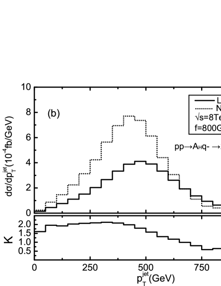
Figure 10: The LO, NLO QCD corrected leading jet transverse momentum distributions and the corresponding $K$ factors for the $pp\to A_{H}q_{-}\to A_{H}A_{H}q+X$ process at the LHC. (a) $\sqrt{s}=14~{}{\rm TeV}$. (b) $\sqrt{s}=8~{}{\rm TeV}$.

The LO, NLO QCD corrected leading jet rapidity distributions and the corresponding $K$ factors for the $pp\to A_{H}q_{-}\to A_{H}A_{H}q+X$ process at the $\sqrt{s}=14$ and $8~{}{\rm TeV}$ LHC are plotted in Figs.11(a) and 11(b), respectively, with $f=800~{}{\rm GeV}$ and $\kappa=1$. From Figs.11(a) and 11(b) we can see that the produced final jets are mainly concentrated in the central rapidity region, and the $K$-factor for the $y^{jet}$ distribution varies slightly in the whole plotted $y^{jet}$ region.

Figure 11: The LO, NLO QCD corrected leading jet rapidity distributions and the corresponding $K$ factors for the $pp\to A_{H}q_{-}\to A_{H}A_{H}q+X$ process at the LHC. (a) $\sqrt{s}=14~{}{\rm TeV}$. (b) $\sqrt{s}=8~{}{\rm TeV}$.

Recently the CMS Collaboration collected the events containing an energetic jet and an imbalance in transverse momentum at the $\sqrt{s}=8~{}{\rm TeV}$ LHC with an integrated luminosity of $19.5~{}fb^{-1}$. It is found that the data are in good agreement with expected contributions from SM processes [38]. In Table 8 of Ref.[38] the expected and observed $95\%$ C.L. upper limits on possible contributions from new physics passing the selection requirements are given. If we take the LHT signal as a single jet event of the $pp\to A_{H}q_{-}\to 2A_{H}q+X$ process. Our calculation of the LHT signal process show that under the present constraint on the scale $f$ the LHT signal does not have significant impact on the present mono-jet event phenomenology. For example, if we take $f=700~{}{\rm GeV}$, $\kappa=1$ and $\mu=\mu_{0}$, we obtain less than three events of the LHT signal passing the cut of $E^{miss}_{T}>500~{}{\rm GeV}$ at the $\sqrt{s}=8~{}{\rm TeV}$ LHC with integrated luminosity of $19.5~{}fb^{-1}$, which is far below the $135$ events of the observed $95\%$ C.L. upper limits on possible contributions from new physics passing the selection cuts.

In order to determine the event selection strategy in further data analysis, we compare the kinematic distributions of the LHT signal and SM background in the following discussion. When we choose the LHT signal as the $A_{H}q_{-}$ production followed by the $q_{-}\to A_{H}q$ decay, i.e., $pp\to A_{H}q_{-}\to 2A_{H}q+X$, its main SM background comes from the $pp\to Z+jet\to\nu\bar{\nu}+jet+X$ process with single jet detected. We plot the NLO QCD corrected distributions of the leading jet $p_{T}$ and the imbalance in transverse momentum for the signal process $pp\to A_{H}q_{-}\to 2A_{H}q+X$, and the LO distributions of $p_{T}^{jet}$ and $p_{T}^{miss}$ for the main SM background process $pp\to Z+jet\to\nu\bar{\nu}+jet+X$ at the $\sqrt{s}=14$ and $8~{}{\rm TeV}$ LHC in Figs.12(a) and 12(b), respectively. From those two figures, we can see that the final leading jet and undetectable particles of the SM background process $pp\to Z+jet\to\nu\bar{\nu}+jet+X$ tend to concentrate in the low $p_{T}$ region, while the final leading jet and undetectable particles of the signal process prefer to be produced in the larger $p_{T}$ region compared with those of the background process. Therefore, it is possible that the SM background from the $pp\to Z+jet\to\nu\bar{\nu}+jet+X$ process can be suppressed if we take appropriate transverse momentum cuts on final leading jet or missing energy.

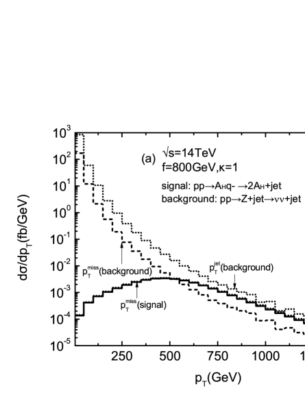
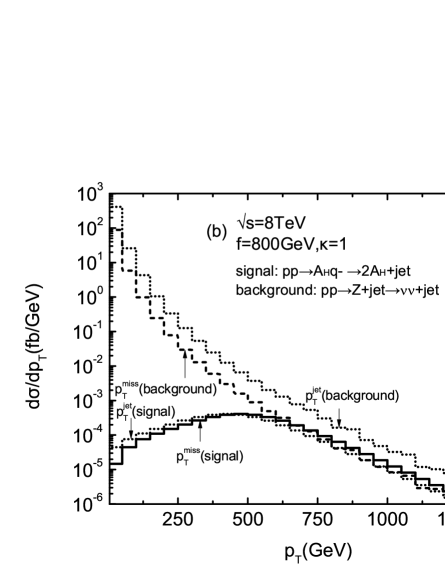
Figure 12: The transverse momentum distributions for the signal process $pp\to A_{H}q_{-}\to 2A_{H}q+X$ and the main SM background process $pp\to Z+jet\to\nu\bar{\nu}+jet+X$ at the LHC. (a) $\sqrt{s}=14~{}{\rm TeV}$. (b) $\sqrt{s}=8~{}{\rm TeV}$.

If we consider the processes $pp\to A_{H}q_{-}\to A_{H}W_{H}q^{\prime}\to 2A_{H}Wq^{\prime}\to 2A_{H}l\nu q^{\prime}+X$ ($l=e,\mu,\tau$) and $pp\to A_{H}q_{-}\to A_{H}Z_{H}q\to 2A_{H}Hq\to 2A_{H}\tau^{+}\tau^{-}q+X$ as the LHT signals, these signals could be detected as the lepton$+$jet$+$missing energy and $2\tau+$jet$+$missing energy events, separately. The corresponding SM backgrounds mainly come from the $pp\to W+jet\to l\nu+jet+X$ ($l=e,\mu,\tau$) and $pp\to W^{+}W^{-}+jet\to\nu_{\tau}\bar{\nu}_{\tau}\tau^{+}\tau^{-}+jet+X$, respectively. We plot the transverse momentum distributions of the final leading jet, lepton and undetectable particles of the signal process $pp\to A_{H}q_{-}\to 2A_{H}l\nu q+X$ and its main SM background process $pp\to W+jet\to l\nu+jet+X$ in Fig.13(a) for the $14~{}{\rm TeV}$ LHC and Fig.13(b) for the $8~{}{\rm TeV}$ LHC. And the signal process $pp\to A_{H}q_{-}\to 2A_{H}\tau^{+}\tau^{-}q+X$ and the corresponding main SM background process $pp\to W^{+}W^{-}+jet\to\nu_{\tau}\bar{\nu}_{\tau}\tau^{+}\tau^{-}+jet+X$ at the $\sqrt{s}=14~{}{\rm TeV}$ and $8~{}{\rm TeV}$ LHC are depicted in Figs.14(a) and 14(b), separately. From the plots in Figs.13(a)-13(b) and Figs.14(a)-14(b), we can find that the transverse momentum distributions of the final leading jet and the undetectable particles of the signal are different with those of background, because the kinematics of the signal is distinctively different from that of background. The leading jet and the undetectable particles in signal prefer to be distributed in the relatively large $p_{T}$ region except the final lepton and $\tau$, while the corresponding distributions of the background events are concentrated in the low $p_{T}$ area. The $p_{T}$ distributions of final lepton and $\tau$ for the signal processes in Figs.13 and Figs.14 show a little special characteristic whose $p_{T}$ distribution shapes are similar with the corresponding ones for the SM backgrounds. From all the six plots we can conclude that if we take some proper cuts on final jet and missing energy, the SM background of the LHT signal could be significantly suppressed.

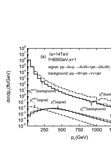
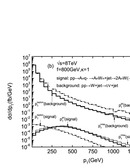
Figure 13: The transverse momentum distributions for the signal process $pp\to A_{H}q_{-}\to A_{H}W_{H}q^{\prime}\to 2A_{H}Wq^{\prime}\to 2A_{H}l\nu q^{\prime}+X$ ($l=e,\mu,\tau$) and the main SM background process $pp\to W+jet\to l\nu+jet+X$ ($l=e,\mu,\tau$) at the LHC. (a) $\sqrt{s}=14~{}{\rm TeV}$. (b) $\sqrt{s}=8~{}{\rm TeV}$.

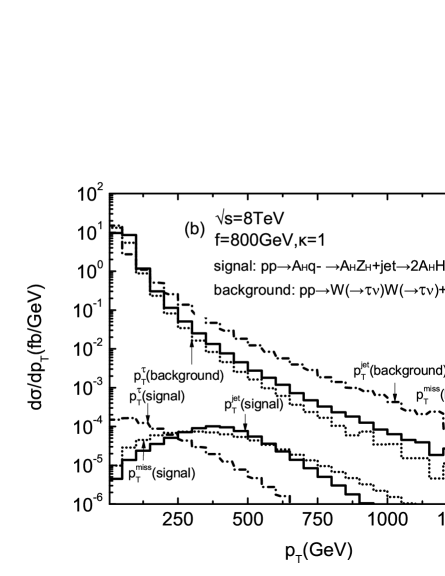
Figure 14: The transverse momentum distributions for the signal process $pp\to A_{H}q_{-}\to A_{H}Z_{H}q\to A_{H}A_{H}Hq\to 2A_{H}\tau^{+}\tau^{-}q+X$ and the main SM background process $pp\to W^{+}W^{-}+jet\to\nu\bar{\nu}\tau^{+}\tau^{-}+jet+X$ at the LHC. (a) $\sqrt{s}=14~{}{\rm TeV}$. (b) $\sqrt{s}=8~{}{\rm TeV}$.

V. Summary

In this paper, we calculate the $A_{H}q_{-}$ $(q_{-}=u_{-},c_{-},d_{-},s_{-},\bar{u}_{-},\bar{c}_{-},\bar{d}_{-},\bar{s}_{-})$ associated production rate at the $\sqrt{s}=14$ and $8~{}{\rm TeV}$ LHC up to the QCD NLO including the subsequent decay $q_{-}\to A_{H}q$ in the littlest Higgs model with $T$parity. We adopt the PROSPINO strategy in real light-quark emission processes to avoid double counting and provide reliable NLO QCD corrected predictions. We investigate the dependence of the integrated cross section on the factorization and renormalization scale $\mu$, the global symmetry breaking scale $f$, and the $T$-odd mirror quark Yukawa coupling $\kappa$. The distributions up to QCD NLO accuracy of the missing transverse momentum, leading jet transverse momentum and rapidity are also provided. Our numerical results show that the NLO QCD correction enhances the LO integrated cross section remarkably with the $K$ factor varying in the range of $1.41\sim 1.68$ ($1.58\sim 1.89$) as the increment of the global symmetry-breaking scale $f$ from $500~{}{\rm GeV}$ to $1.5~{}{\rm TeV}$ ($1.1~{}{\rm TeV}$) at the $\sqrt{s}=14~{}{\rm TeV}$ ($8~{}{\rm TeV}$) LHC. We also analyze the distributions of the transverse momenta of final particles of the LHT signals and their SM backgrounds, and find that it is possible to select the signal events of the $A_{H}q_{-}$ production from its background by taking proper cuts on the final leading jet and missing energy.

Acknowledgments: This work was supported in part by the National Natural Science Foundation of China (Grants. No.11075150, No.11275190, No. 11375008), and the Fundamental Research Funds for the Central Universities (Grant. No.WK2030040024). X.-D. Yang would like to acknowledge support by the Fund for Fostering Talents in Basic Science of the National Natural Science Foundation of China (No.J1103207).

References

- [1] S. L. Glashow, Nucl. Phys. 22 (1961) 579; S. Weinberg, Phys. Rev. Lett. 19 (1967) 1264; A. Salam, Proc. 8th Nobel Symposium Stockholm 1968,ed. N. Svartholm (Almquist and Wiksells, Stockholm 1968) p.367; H. D. Politzer, Phys. Rept. 14 (1974) 129.
- [2] P. W. Higgs, Phys. Lett. 12 (1964) 132, Phys. Rev. Lett. 13 (1964) 508, Phys. Rev. 145 (1966) 1156; F. Englert and R. Brout, Phys. Rev. Lett. 13 (1964) 321; G. S. Guralnik, C. R. Hagen and T. W. B. Kibble, Phys. Rev. Lett. 13 (1964) 585; T. W. B. Kibble, Phys. Rev. 155 (1967) 1554.
- [3] R. Barbieri and A. Strumia, IFUP-TH/2000-22 and SNS-PH/00-12, [arXiv:hep-ph/0007265].
- [4] S. P. Martin, arXiv:hep-ph/9709356; M. E. Peskin, arXiv:0801.1928 [hep-ph]; K. A. Olive, arXiv:hep-ph/9911307; M. Drees, arXiv:hep-ph/9611409; H. E. Haber and G. L. Kane, Phys. Rept. 117 (1985) 75; H. P. Nilles, Phys. Rept. 110, 1 (1984); A. Signer, J.Phys.G36 (2009) 073002, arXiv:0905.4630 [hep-ph].
- [5] N. Arkani-Hamed, S. Dimopoulos, G. Dvali, Phys. Lett. B429 (34): 263(1998), arXiv:hep-ph/9803315; N. Arkani-Hamed, S. Dimopoulos, G. Dvali, Phys. Rev. D59 086004(1999), arXiv:hep-ph/9807344; I. Antoniadis, N. Arkani-Hamed, S. Dimopoulos, G. Dvali, Phys. Lett. B436 (34): 257(1998), arXiv:hep-ph/9804398; M. Shifman, Int. J. Mod. Phys. A25 199-225,2010, arXiv:0907.3074v2 [hep-ph].
- [6] N. Arkani-Hamed, A. G. Cohen and H. Georgi, Phys. Lett. B513 (2001) 232; M. Schmaltz and D. Tucker-Smith, Ann. Rev. Nucl. Part. Sci. 55 (2005) 229; M. Perelstein, Prog. Part. Nucl. Phys. 58 (2007) 247; and references therein.
- [7] G.G. Ross, ”Grand Unified Theories” (Addison-Wesley Publishing Company, Reading, MA, (1984); P. Langacker, Phys. Rep. 72 (1981) 185; H. Georgi, S.L Glashow, Phys. Rev. Lett. 32 (1974) 438; A.J. Buras, J. Ellis, M.K. Gaillard, D.V. Nanopoulos, Nucl. Phys. B135(1978) 66.
- [8] Arkani-Hamed, A. G. Cohen, E. Katz, A. E. Nelson, T. Gregoire and J. G. Wacker, JHEP 08 (2002) 021.
- [9] T. Gregoire and J. G. Wacker, JHEP 08 (2002) 019.
- [10] N. Arkani-Hamed, A. G. Cohen, E. Katz and A. E. Nelson, JHEP 07 (2002) 034.
- [11] C. Csaki, J. Hubisz, G. D. Kribs, P. Meade and J. Terning, Phys. Rev. D 67 (2003) 115002; J. L. Hewett, F. J. Petriello and T. G. Rizzo, JHEP 10 (2003) 062; C. Csaki, J. Hubisz, G. D. Kribs, P. Meade and J. Terning, Phys. Rev. D68 (2003) 035009; M. -C. Chen and S. Dawson, Phys. Rev. D70 (2004) 015003; W. Kilian and J. Reuter, Phys. Rev. D70 (2004) 015004; Z. Han and W. Skiba, Phys. Rev. D71 (2005) 075009.
- [12] Jurgen Reuter , Marco Tonini , Maikel de Vries,’Little Higgs Model Limits from LHC - Input for Snowmass 2013’, arxiv:1307.5010;’Littlest Higgs with T-parity: Status and Prospects’, arXiv:1310.2918.
- [13] L. Wang, J.-M. Yang, and J.-Y. Zhu, ’Dark matter in little Higgs model under current experimental constraints from LHC, Planck and Xenon’, arXiv:1307.7780v1.
- [14] I. Low, JHEP 10 (2004) 067.
- [15] H. -C. Cheng and I. Low, JHEP 09 (2003) 051, JHEP 08 (2004) 061.
- [16] J. Hubisz, P. Meade, A. Noble and M. Perelstein, JHEP 01 (2006) 135.
- [17] A. Birkedal, A. Noble, M. Perelstein and A. Spray, Phys. Rev. D74 (2006) 035002; M. Asano, S. Matsumoto, N. Okada, and Y. Okada, Phys. Rev. D75 (2007) 063506.
- [18] A. Belyaev, C. -R. Chen, K. Tobe and C. -P. Yuan, Phys. Rev. D74, (2006) 115020.
- [19] M. Blanke, A. J. Buras, A. Poschenrieder, S. Recksiegel, C Tarantino, S. Uhliga and A. Weilera, JHEP01(2007)066; J. Hubisz, S. J. Leeb and G. Pazb, JHEP06(2006)041; J. Hubisz and P. Meade, Phys. Rev. D71, 035016 (2005).
- [20] A. Belyaev, C. -R. Chen, K. Tobe and C. -P. Yuan, in Proceedings of Monte Carlo Tools for Beyond the Standard Model Physics, Fermilab, 2006, given by A. Belyaev, http://theory.fnal.gov/mc4bsm/agenda.html; in Proceedings of Osaka University, 2006, Osaka, given by C. -P. Yuan, http://www-het.phys.sci.osaka-u.ac.jp/seminar/seminar/seminar.html; in Proceedings of the Summer Institute on Collider Phenomenology, National Tsing Hua University, Taiwan, 2006, given by K. Tobe, http://charm.phys.nthu.edu.tw/hep/summer2006/; in Proceedings of ICHEP’06, Moscow, 2006, (World Scientific, Singapore, 2006).
- [21] J. Hubisz and P. Meade, Phys. Rev. D71 (2005) 035016.
- [22] J. Hubisz, S. -J. Lee and G. Paz, JHEP 06 (2006) 041.
- [23] M. Blanke, A. J. Buras, A. Poschenrieder, S. Recksiegel, C. Tarantino, S. Uhlig and A. Weiler JHEP 01 (2007) 066.
- [24] R.-Y. Zhang, Y. Han, W.-G. Ma, S.-M. Wang, L. Guo, and L. Han, Phys. Rev. D85(2012) 015017.
- [25] J. Hubisz and P. Meade, Phys. Rev. D71, 035016 (2005).
- [26] J. Hubisz, P. Meade, A. Noble and M. Perelstein, JHEP 0601, 135 (2006).
- [27] T. Hahn, Comput. Phys. Commun. 140, 418 (2001).
- [28] T. Hahn and M. Perez-Victoria, Comput. Phys. Commun. 118, 153 (1999).
- [29] J. Collins, F. Wilczek, and A. Zee, Phys. Rev. D18 (1978) 242; W. J. Marciano, Phys. Rev. D29 (1984) 580; P. Nason, S. Dawson and R.K. Ellis, Nucl. Phys. B327 (1989) 49, Nucl. Phys. B335 (1990) 260(E).
- [30] B. W. Harris and J. F. Owens, Phys. Rev. D65 (2002) 094032.
- [31] T. Kinoshita, J. Math. Phys. 3 (1962) 650; T. D. Lee and M. Nauenberg, Phys. Rev. 133 (1964) B1549.
- [32] W. Beenakker, R. Höpker, M. Spira and P. M. Zerwas, Nucl. Phys. B492 (1997) 51; W. Beenakker, M. Klasen, M. Krämer, T. Plehn, M. Spira and P. M. Zerwas, Phys. Rev. Lett. 83 (1999) 3780; http://www.thphys.uni-heidelberg.de/~plehn/index.php?show=prospino.
- [33] T. Plehn and C. Weydert, PoS CHARGED2010 (2010) 026, [arXiv:1012.3761]; T. Binoth, D. Goncalves-Netto, D. Lopez-Val, K. Mawatari, T. Plehn and I. Wigmore, Phys. Rev. D84 (2011) 075005, [arXiv:1108.1250].
- [34] J. Pumplin, D. R. Stump, J. Huston, H. -L. Lai, P. Nadolsky and W. -K. Tung, JHEP 07 (2002) 012; D. Stump, J. Huston, J. Pumplin, W. -K. Tung, H. -L. Lai, S. Kuhlmann and J. F. Owens, JHEP 10 (2003) 046.
- [35] Particle Data Group, J. Beringer et al, phys. Rev. D86 (2012) 010001
- [36] S.-M. Du, L. Lei, W. Liu, W.-G. Ma, and R.-Y. Zhang, Phys. Rev. D 86, (2012) 054027.
- [37] S.D. Ellis and D.E. Soper, Phys. Rev. D48,3160(1993), arXiv:hep-ph/9305266.
- [38] The CMS Collaboration, ”Search for new physics in monojet events in pp collisions at ”, CMS PAS EXO-12-048.