Quantum $s=1/2$ Antiferromagnets on Archimedean Lattices: The Route from Semiclassical Magnetic Order to Nonmagnetic Quantum States

Abstract

We investigate ground states of $s$=1/2 Heisenberg antiferromagnets on the eleven two-dimensional (2D) Archimedian lattices by using the coupled cluster method. Magnetic interactions and quantum fluctuations play against each other subtly in 2D quantum magnets and the magnetic ordering is thus sensitive to the features of lattice topology. Archimedean lattices are those lattices that have 2D arrangements of regular polygons and they often build the underlying magnetic lattices of insulating quasi-two-dimensional quantum magnetic materials. Hence they allow a systematic study of the relationship between lattice topology and magnetic ordering. We find that the Archimedian lattices fall into three groups: those with semiclassical magnetic ground-state long-range order, those with a magnetically disordered (cooperative quantum paramagnetic) ground state, and those with a fragile magnetic order. The most relevant parameters affecting the magnetic ordering are the coordination number and the degree of frustration present.

In two-dimensional (2D) quantum Heisenberg antiferromagnets (HAFMs) the balance between quantum fluctuations and interactions depends subtly on the topology of the underlying lattice. Thus, a large variety of ground state (GS) phases are found in 2D quantum magnets, among them exotic quantum states, see, e.g., balents ; sachdev . The prototypes of 2D arrangements of spins are the 11 uniform Archimedean lattices (ALs), see, e.g., gruenbaum ; ed_archimedean , which present an ideal playground for a systematic study of the interplay between lattice topology, magnetic interactions and quantum fluctuations. ALs are formed from 2D arrangements of regular polygons. Moreover, all sites of a certain AL are topologically equivalent, but the nearest-neighbor (NN) bonds are allowed to be topologically inequivalent. Well-known (and well studied) members of the ALs are the square, honeycomb, triangular, and kagome lattices. More exotic (and less studied) lattices are the star, “CaVO”, “SHD”, maple-leaf, trellis, “SrCuBO” and bounce lattices, see, e.g., Fig. 1.

Four of the ALs (namely square, honeycomb, CaVO, and SHD) are bipartite lattices (i.e. only even polygons are present). In the other seven ALs triangular polygons are present and the HAFM is frustrated. In particular, the triangular and the kagome lattices have attracted much attention as paradigms of 2D frustrated lattices, see, e.g., Refs. dmrg_trian, ; zhito2009, ; tanaka, ; mendels, ; Yan2011, ; lauchli2011, ; scholl, ; kagome_general_s, ; normand2013, . Interestingly, not only the well-known ALs are found to be underlying lattice structures of the magnetic ions of various compounds, but also the more exotic ones are realized, see, e.g., CaV₄O₉ (CaVO) Tan , SrCu₂(BO₃)₂ (SrCuBO) Kag , a polymeric iron(III) acetate (star)star or $\mathrm{M_{x}}[\mathrm{Fe}(\mathrm{O}_{2}\mathrm{CCH}_{2})_{2}\mathrm{NCH}_{2}\mathrm{PO}_{3}]_{6}\cdot\mathrm{nH}_{2}\mathrm{O}$ and Cu₆Al(SO₄)(OH)₁₂Cl$\cdot$3H₂O (maple-leaf)cave ; fennell . Very recently, an overview of the experimental realizations of Archimedean spin lattice materials (and from the point-of-view of a chemist) has been given in Ref. [Zheng, ]. Hence, a systematic and comparative investigation of the HAFM on the ALs is not only interesting as a “paradigmatic” study of the role of topology in 2D quantum systems but also from the experimental point of view in the field of quantum magnetism. Let us also mention here, that the special lattice topology of the ALs plays a role in a large variety of interacting quantum system such as Chern insulators, see e.g. Refs. fiete2011, ; bernevig2012, , or chiral spin liquids, see e.g. Ref. kivelson2007, .

Figure 1: The eleven Archimedean lattices.

A first attempt to study the GS properties systematically was given in Ref. ed_archimedean, where exact diagonalization (ED) data for the GS energies and order parameters for the spin-1/2 HAFM on the ALs were presented. ED is severely limited by the maximum lattice size that can be treated by using even very large computational resources starI ; ED40 ; lauchli2011 . Since only two of the ALs are primitive lattices with only one site per geometric unit cell (namely square and triangular) one may therefore only have two or three points to extrapolate to the infinite-lattice limit ed_archimedean . We mention, that due to the sign problemTrWi05 frustrated quantum magnets cannot be treated adequately by efficient Quantum Monte Carlo (QMC) techniques. Hence, a clear picture regarding the existence of GS magnetic long-range order (LRO) for some of the ALs has yet to emerge.

In this paper we analyze the GS energy $E_{g}$ and the magnetic order parameter (sublattice magnetization) $M$ of the HAFM on all of the ALs for the extreme quantum case, i.e. spin quantum number $s=1/2$, by using the coupled-cluster method (CCM). The corresponding Hamiltonian is given by

$$H=J\sum_{\langle i,j\rangle}{\bf s}_{i}\cdot{\bf s}_{j}\;.$$ (1)

The symbol $\langle i,j\rangle$ indicates those bonds connecting NN sites (counting each bond once only) on all of the ALs. We set the energy scale by putting $J=1$.

We illustrate here only some relevant features of the CCM. For more general information on the methodology of the CCM, see, e.g., Refs. ccm_theory, ; zeng98, ; bishop98a, ; bishop04, . CCM has recently been applied computationally at high orders of approximation to quantum magnetic systems with much success, see, e.g., Refs. spin_systems_book ; spin_half_xxz ; ccm_j_prime ; ccm_shastry ; ccm_extra ; ccm_maple ; kagome_general_s . In the field of quantum magnetism, advantages of this approach are that it can be applied to strongly frustrated quantum spin systems in any dimension and with arbitrary spin quantum numbers.

A basic element of the single-reference CCM used here is the parameterization the ket GS eigenvector $|\Psi\rangle$ of a general many-body system described by a Hamiltonian $H$ (where $H|\Psi\rangle=E_{g}|\Psi\rangle$) via $|\Psi\rangle={\rm e}^{S}|\Phi\rangle$ and where $S=\sum_{I\neq 0}{\cal S}_{I}C_{I}^{+}$. For spin systems the model or reference state $|\Phi\rangle$ is related to the classical GS and the many-body creation operators $C_{I}^{+}$ applied to $|\Phi\rangle$ can be expressed by appropriate products of spin-flip operators spin_systems_book ; spin_half_xxz ; ccm_j_prime ; ccm_shastry ; ccm_extra ; ccm_maple ; kagome_general_s . For the unfrustrated “bipartite” lattices (namely, square, CaVO, SHD, and honeycomb), the model state $|\Phi\rangle$ is taken to be the classical collinear two-sublattice Néel GS. For the frustrated “non-bipartite” lattices (namely, triangular, kagome, star, maple-leaf, trellis, SrCuBO, and bounce), non-collinear classical GSs are typical. An exception is the SrCuBO lattice, which has a pattern of exchange bonds that is topologically equivalented_archimedean to the famous Shastry-Sutherland model Shastry . For this frustrated model also the collinear two-sublattice Néel ground state is appropriate as our model state ed_archimedean ; Mila ; ccm_shastry . For the triangular lattice we have the well-known 120^∘ three-sublattice state. For the maple-leaf and bounce lattices the classical GS used as model state has six sublattices with a characteristic pitch angle ed_archimedean ; ccm_maple . The classical GS of the trellis lattice is an incommensurate spiral one along a chain ed_archimedean ; trellis . As quantum fluctuations may lead to a “quantum” pitch angle that deviates from the classical one ccm_j_prime ; ccm_shastry , we consider the pitch angle in the model states of the maple-leaf, bounce and trellis lattices as a free parameter. The case for the kagome and star lattices is more subtle as there are an infinite number of possible classical ground states to choose from. However, current understanding is that quantum fluctuations favor of coplanar states for these systems, such as $\sqrt{3}\times\sqrt{3}$ and $q=0$ states ed_archimedean ; chub92 ; henley1995 ; sachdev1992 , which are used here as model states.

To perform the CCM calculations for quantum many-body problems one has naturally to use approximations. Here we utilize the LSUB$m$ approximation scheme, in which all $m$-body clusters spanning a range of no more than $m$ adjacent lattice sites are retained (for details, see Refs. spin_systems_book, ; spin_half_xxz, ; ccm_j_prime, ; ccm_shastry, ; ccm_extra, ; ccm_maple, ; kagome_general_s, ). To analyze the GS magnetic LRO we consider the sublattice magnetization $M(m)$ that can be straightforwardly calculated within a certain CCM-LSUB$m$ approximation spin_systems_book ; ccm_j_prime ; ccm_shastry . For more information about the definition of the order parameter $m^{+}$ used in the ED study of the ALs in Ref. ed_archimedean, , see pages 93 to 94 of that reference.

Table 1: Extrapolated CCM results for the GS energy per bond of the spin-1/2 HAFM on the various Archimedean lattices compared to ED results from Ref. ed_archimedean and other available data. (Results for the star and kagome lattices are given for the $q=0$ and $\sqrt{3}\times\sqrt{3}$ model states.)

Lattice	CCM	ED (Ref.ed_archimedean, )	other results
Bipartite
square	$-0.3348$	$-$0.3350	$-$0.3347 [sandvik97, ]
honeycomb	$-0.3631$	$-$0.3632	$-$0.3630 [reger89, ]
CaVO	$-0.3689$	$-$0.3689	$-$0.3691 [spin_half_cavo_II, ]
SHD	$-0.3702$	$-$0.3713	$-$0.3688 [shd, ]
Frustrated
SrCuBO	$-0.2312$	$-$0.2310	$-0.23\ldots 0.24$ [Mila2013, ]
triangular	$-0.1843$	$-$0.1842	$-$0.1823 [zhito2009, ]
bounce	$-0.2824$	$-$0.2837
trellis	$-0.2416$	$-$0.2471
maple-leaf	$-0.2124$	$-$0.2171
kagome		$-0.2172$	$-0.2190\ldots 0.2193$ [Yan2011, ; scholl, ]
$q=0$	$-$0.2179
$\sqrt{3}\times\sqrt{3}$	$-$0.2159
star		$-0.3093$	$-0.316\ldots 0.318$ [starIII, ]
$q=0$	$-$0.3110
$\sqrt{3}\times\sqrt{3}$	$-$0.3101

Table 2: Extrapolated CCM results for the order parameter $M$ (of the spin-1/2 HAFM on the various Archimedean lattices compared to ED results from Ref. ed_archimedean and other available data. (Results for the star and kagome lattices are given for the $q=0$ and $\sqrt{3}\times\sqrt{3}$ model states. )

Lattice	CCM	ED (Ref.ed_archimedean, )	other results
Bipartite
square	0.619	0.635	0.614…0.617 [sandvik97, ; wiese1996, ]
honeycomb	0.547	0.558	0.535 [spin_half_honeycomb, ]
CaVO	0.431	0.461	0.356 [spin_half_cavo_I, ]
SHD	0.366	0.425	0.509 [shd, ]
Frustrated
SrCuBO	0.404	0.456	0.42 [Mila2013, ]
triangular	0.373	0.386	0.410 [dmrg_trian, ]
bounce	$M_{I}$: 0.122	0.286
	$M_{II}$: $0$
trellis	$M_{I}$: 0.040	0.222
	$M_{II}$: $0$
maple-leaf	$M_{I}$: 0.178	0.218
	$M_{II}$: $0$
kagome			0
$q=0$	$0$
$\sqrt{3}\times\sqrt{3}$	$0$
star		0.094…0.15
$q=0$	$0$
$\sqrt{3}\times\sqrt{3}$	$0$

Since the LSUB$m$ approximation becomes exact only in the limit $m\rightarrow\infty$, it is useful to extrapolate the LSUB$m$ results in this limit. For the GS energy the extrapolation scheme $E_{g}(m)/N=E_{g}(m=\infty)/N+a_{1}/m^{2}+a_{2}/m^{4}$ is well-establishedspin_systems_book ; spin_half_xxz ; ccm_j_prime ; ccm_shastry ; ccm_extra ; ccm_maple ; kagome_general_s . For the magnetic order parameter $M$ the choice of an appropriate extrapolation scheme is more subtle. In cases where GS magnetic LRO is present, e.g. for the square lattice, the scheme I with $M(m)=M_{\rm I}(m=\infty)+b_{1}/m+b_{2}/m^{2}$ leads to excellent results for the order parameterspin_systems_book ; spin_half_xxz . On the other hand, for systems where the GS magnetic LRO is unstable, the scheme II with $M(m)=M_{\rm II}(m=\infty)+c_{1}/m^{1/2}+c_{2}/m^{3/2}$ is favorableccm_extra ; kagome_general_s . It is also well-known that low-level LSUB$m$ approximations are poor approximations, and they do not follow the extrapolation rules well. Hence, LSUB2 and LSUB3 data are excluded from extrapolation. Moreover, since for collinear model states (i.e. for bipartite square, honeycomb, CaVO, SHD lattices and for the SrCuBO lattice) no odd-numbered spin flips appearspin_systems_book ; spin_half_xxz , we take into account in the extrapolation for these lattices only LSUB$m$ data with even $m\geq 4$. On the other hand, for the triangular, kagome, star, maple-leaf, trellis, and bounce lattices where we use non-collinear model states (i.e. odd-numbered spin flips appear) we take into account in the extrapolation all LSUB$m$, $m\geq 4$ comment . Due to the different complexity of the lattices and the corresponding model states the maximum level $m_{\rm max}$ of LSUB$m$ approximations accessible within our CCM code is not unique. Thus, we have $m_{\rm max}=12$ for the square, honeycomb, CaVO, SHD, $m_{\rm max}=10$ for the triangular, kagome, star, SrCuBO, and $m_{\rm max}=8$ for the bounce, maple-leaf, and trellis lattices.

To decide, which extrapolation for the order parameter is appropriate we proceed as follows: First we apply both extrapolation schemes I and II. In case that both schemes lead to $M_{\rm I}(m=\infty)>0$ and $M_{\rm II}(m=\infty)>0$ we have evidence for GS magnetic LRO, and we use scheme I for further consideration. In case that both schemes lead to vanishing $M_{\rm I}(m=\infty)$ and $M_{\rm II}(m=\infty)$, we have clear evidence for the breakdown of GS magnetic LRO. However, there are also some cases, where $M_{\rm I}(m=\infty)>0$ but $M_{\rm II}(m=\infty)$ vanishes, see table 2. Although, in these cases a clear statement about GS magnetic LRO is problematic the magnetic LRO is at least very fragile, and a non-magnetic cooperative quantum paramagnetic GS is likely.

It is appropriate to mention earlier attempts to calculate the GS quantities by means of the CCM for some of the ALs, namely Refs. spin_half_xxz, ; ccm_square, (square), Ref. ccm_trian, (triangular), Ref. ccm_j_prime, (honeycomb), Ref. ccm_cavo, (CaVO), Ref. kagome_general_s, (kagome), Ref. ccm_maple, (maple-leaf), and Ref. ccm_maple, (bounce). However, most of these previous calculations are limited to lower levels of approximation LSUB$m$. Hence the new data using higher LSUB$m$ presented here may yield much more accurate results.

We collect our CCM results for E in Table 1 and for M in Table 2. These are compared to those results for the ground-state energies and order parameters $M$ quoted on page 118 of Ref. ed_archimedean, . Moreover we also present available data from previous investigations using other methods.

All the bipartite ALs (and so for unfrustrated HAFM systems) exhibit magnetic LRO, where the order parameter is significantly reduced by quantum fluctuations. This reduction is strongest for the two lattices with non-equivalent NN (CaVO and SHD), indicating a possible instability against a non-magnetic valence-bond state spin_half_cavo_I . Thus the order parameter for the SHD lattice is only $37$% of the classical value. Note that our data for the bipartite square, honeycomb and CaVO lattices are in good agreement with available QMC datasandvik97 ; wiese1996 ; spin_half_honeycomb ; spin_half_cavo_I ; spin_half_cavo_II , which can be considered as benchmark results. For the bipartite SHD lattice no QMC data are published, the results reported in Ref. shd, are obtained by a variational technique that might be less accurate than our high-order CCM results.

For the frustrated lattices the QMC cannot serve as benchmark approach. Hence, typically the previously published results may have limited accuracy and our high-order CCM data contribute to a refinement of the GS data and a better understanding of these frustrated quantum HAFMs. The reference data quoted in Tables 1 and 2 are obtained by tensor-network approachMila2013 , spin-wave theoryzhito2009 , density-matrix renormalization group methodYan2011 ; scholl ; dmrg_trian , and bond-operator techniquestarIII . Among the frustrated ALs the SrCuBO lattice is special, since it is the only lattice having a classical collinear Néel GS. Hence it is not surprising that the quantum GS possesses Néel LRO with the largest order parameter $M$ of the frustrated ALs. However, the effect of frustration is obvious by a noticeably reduced $M$ compared to the square lattice.

Particular attention has been paid in the literature to the famous kagome HAFM mendels ; Yan2011 ; lauchli2011 ; scholl ; kagome_general_s ; normand2013 . The good agreement of the CCM GS energy given in Table 1 with recent large-scale density-matrix renormalization groupYan2011 ; scholl , exact-diagonalizationlauchli2011 , and tensor-network approachnormand2013 results gives an indication of the accuracy of our CCM approach for frustrated lattices. Another example for a non-magnetic GS, first mentioned in Ref. ed_archimedean, , is the star-lattice HAFM. For the kagome and the star lattices the two extrapolation schemes yield vanishing order parameters for both model states, $q=0$ and $\sqrt{3}\times\sqrt{3}$, that is consistent with previous studies of these lattices ed_archimedean ; Yan2011 ; lauchli2011 ; scholl ; kagome_general_s ; starI ; starII ; starIII . We mention that for both lattices the CCM GS energy for the $q=0$ model state is lower than that for the $\sqrt{3}\times\sqrt{3}$ model state. That is different from previous studies of the GS selection based on an expansion around the classical limitchub92 ; sachdev1992 ; henley1995 , where for the kagome lattice the $\sqrt{3}\times\sqrt{3}$ state was found to be selected by quantum fluctuations. This may be related to the extreme quantum case of $s=1/2$ considered here that is not well described by an expansion around the classical limit, see also the discussion in Ref. kagome_general_s, .

For the trellis, maple-leaf and bounce lattices the results are less clear, since both extrapolation schemes lead to different conclusions with respect to magnetic LRO. In general, for systems near to a quantum critical point the results may depend on details of both the extrapolation scheme and orders of approximation used commentII . Due to the computational difficulty for these lattices, these extrapolations used LSUB4 to LSUB8 approximations only, the lowest orders of approximation used in this paper, and we find that extrapolation scheme I yields a small but finite order parameter $M$ that is significantly below the ED results reported in Ref. ed_archimedean . By way of comparison, we note that extrapolations using scheme 1 with LSUB5 to LSUB8 indicate that the order parameter is 29% , 21%, and 29% of its classical value for the bounce, trellis, and maple-leaf lattices. Note also that the finite-size extrapolation of the ED data for these lattices is particularly poor, since only two (bounce, maple-leaf) or three (trellis) data points could be used. Moreover, periodic boundary conditions used for ED calculations in Ref. ed_archimedean might be not well-suited for the incommensurate spiral correlations present for the trellis lattice. On the other hand, extrapolation scheme II using LSUB4 to LSUB8 for these three lattices lead to vanishing order parameters. Hence, we may conclude that these lattices exhibit either a weak magnetic LRO or are even in a magnetically disorder GS phase. Hence, they are candidates to find non-magnetic states in experiments, see also Ref.fennell . We mention that in Ref. trellis, by means of spin-wave and variational techniques similar conclusions for the trellis lattice were found.

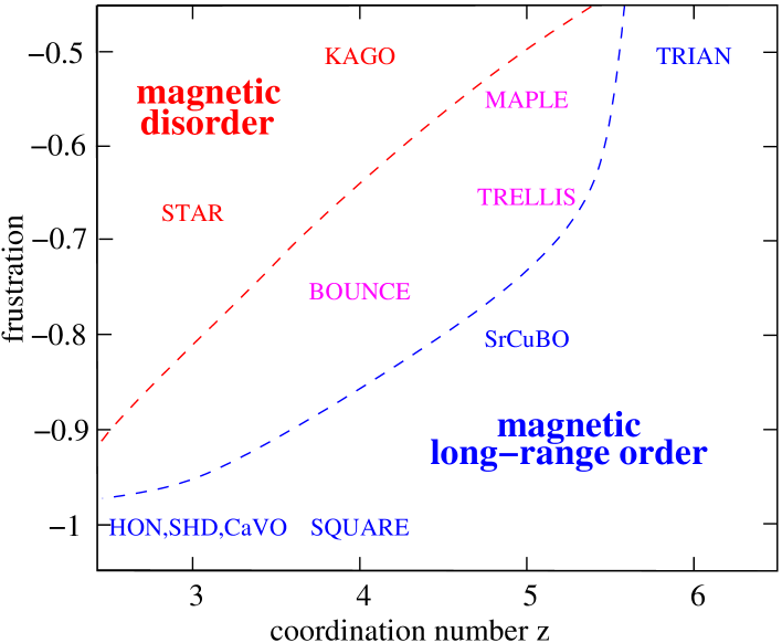
Figure 2: Sketch of semi-classical magnetic order and quantum magnetic disorder of the ALs in a parameter space spanned by frustration (classical GS energy per bond, see Ref. frustration, ) and coordination number $z$.

In this manuscript we have presented a survey of results for ground-state energy and order parameter of the $s=1/2$ Heisenberg antiferromagnet on all eleven Archimedean lattices by using the CCM. In 2D quantum magnets the competition between fluctuations and interaction determines the GS features. Our results show a clear correspondence between lattice topology and existence of GS magnetic LRO. The most important ingredients affecting the magnetic ordering are geometric frustration and the coordination number. Moreover, the competition of non-equivalent NN bonds is relevant. To illustrate the role of geometric frustration and coordination number we summarize our findings in Fig. 2 in a parameter space spanned by frustrationfrustration and coordination number $z$. Clearly there are three regions of magnetic GS ordering: semiclassical magnetic LRO (collinear or non-collinear), magnetic disorder (cooperative quantum paramagnetism) and an intermediate region with ALs, namely trellis, bounce, maple-leaf, which may have either a GS with fragile magnetic LRO, a critical GS order or a GS with weak disorder. This group of ALs deserves particular further attention to clarify the nature of the GSs. We think that our results ought to provide also a useful benchmark for the Archimedean lattices to which experimental studies and other approximate theoretical methods might be tested.

References

- (1) L. Balents, Nature 464, 199 (2010).
- (2) S. Sachdev, arXiv:1203.4565v4 (2012).
- (3) B. Grünbaum, G.C. Shephard, Tilings and Patterns, W.H. Freeman and Company, New York (1987).
- (4) J. Richter, J. Schulenburg, A. Honecker, Lect. Notes Phys. 645, 85-153 (2004).
- (5) J. Richter, J. Schulenburg, A. Honecker, and D. Schmalfuß, Phys. Rev. B 70, 174454 (2004).
- (6) J. Richter and J. Schulenburg, Eur. Phys. J. B 73, 117 (2010).
- (7) A. M. Läuchli, J. Sudan, and E. S. Sørensen, Phys. Rev. B 83, 212401 (2011).
- (8) S. R. White and A. L. Chernyshev, Phys. Rev. Lett. 99, 127004 (2007).
- (9) A. L. Chernyshev and M. E. Zhitomirsky, Phys. Rev. B 79, 144416 (2009).
- (10) Y. Shirata, H. Tanaka, A. Matsuo, and K. Kindo, Phys. Rev. Lett. 108, 057205 (2012); T. Susuki, N. Kurita, T. Tanaka, H. Nojiri, A. Matsuo, K. Kindo, H. Tanaka, Phys. Rev. Lett. 110, 267201 (2013).
- (11) B. Fak, E. Kermarrec, L. Messio, B. Bernu, C. Lhuillier, F. Bert, P. Mendels, B. Koteswararao, F. Bouquet, J. Ollivier, A. D. Hillier, A. Amato, R. H. Colman, A. S. Wills, Phys. Rev. Lett. 109, 037208 (2012).
- (12) S. Yan, D. A. Huse, and S. R. White, Science 332, 1173 (2011); see also arXiv:1011.6114v1 (2010).
- (13) S. Depenbrock, I. P. McCulloch, U. Schollwöck, Phys. Rev. Lett. 109, 067201 (2012).
- (14) O. Götze, D.J.J. Farnell, R.F. Bishop, P.H.Y. Li, and J. Richter, Phys. Rev. B 84, 224428 (2011).
- (15) Z. Y. Xie, J. Chen, J. F. Yu, X. Kong, B. Normand, T. Xiang, arXiv:1307.5696
- (16) T.-P. Choy, Y. B. Kim, Phys. Rev. B 80, 064404 (2009).
- (17) B.-J. Yang, A. Paramekanti, Y. B. Kim, Phys. Rev. B 81, 134418 (2010).
- (18) S. Taniguchi, T. Nishikawa, Y. Yasui, Y. Kobayashi, M. Sato, T. Nishioka, M. Kontani and K. Sano, J. Phys. Soc. Jpn. 64, 2758 (1995).
- (19) H. Kageyama H. Kageyama, K. Yoshimura, R. Stern, N. V. Mushnikov, K. Onizuka, M. Kato, K. Kosuge, C. P. Slichter, T. Goto, and Y. Ueda, Phys. Rev. Lett. 82, 3168 (2000).
- (20) Y.-Z. Zheng, M.-L. Tong, W. Xue, W.-X. Zhang, X.-M. Chen, F. Grandjean, and G. J. Long, Angew. Chem. Int. Ed. 46, 6076 (2007).
- (21) D. Cave, F.C. Coomer, E. Molinos, H.H. Klauss, and P.T. Wood, Angew. Chem. Int. Ed. 45, 803 (2006).
- (22) T. Fennell, J.O. Piatek, R.A. Stephenson, G.J. Nilsen and H.M. Ronnow, J. Phys.: Condens. Matter 23, 164201 (2011).
- (23) Y.Z. Zheng, Z. Zheng, X.M. Chen, Coordination Chemistry Reviews 258-259, 1 (2014).
- (24) X. Hu, M. Kargarian, and G. A. Fiete, Phys. Rev. B 84, 155116 (2011).
- (25) Y.-L. Wu, B.A. Bernevig, and N. Regnault, Phys. Rev. B 85, 075116 (2012).
- (26) H. Yao and S.A. Kivelson, Phys. Rev. Lett. 99, 247203 (2007).
- (27) M. Troyer and U.J. Wiese, Phys. Rev. Lett. 94, 170201 (2005).
- (28) R.F. Bishop, Theor. Chim. Acta 80, 95 (1991).
- (29) C. Zeng, D. J. J. Farnell, and R. F. Bishop, J. Stat. Phys. 90, 327 (1998).
- (30) R. F. Bishop, in Microscopic Quantum Many-Body Theories and Their Applications, edited by J. Navarro and A. Polls, Lecture Notes in Physics 510 (Springer, Berlin, 1998), p.1.
- (31) D. J. J. Farnell and R. F. Bishop, in Quantum Magnetism, Lecture Notes in Physics 645, edited by U. Schollwöck, J. Richter, D. J. J. Farnell, and R. F. Bishop (Springer, Berlin, 2004), p. 307.
- (32) J. B. Parkinson and D. J. J. Farnell. An Introduction To Quantum Spin Systems. Lecture Notes In Physics 816. (Springer Verlag, 2010).
- (33) R.F. Bishop, D.J.J. Farnell, S.E. Krüger, J.B. Parkinson, J. Richter and C. Zeng, J. Phys.: Condens. Matter 12 6887 (2000).
- (34) S.E. Krüger, J. Richter, J. Schulenburg, D.J.J. Farnell and R.F. Bishop, Phys. Rev. B 61, 14607 (2000).
- (35) R. Darradi, J. Richter, and D. J. J. Farnell, Phys. Rev. B 72, 104425 (2005).
- (36) R.F. Bishop, P.H.Y. Li, R. Darradi, and J. Richter, J. Phys.: Condens. Matter 20, 255251 (2008).
- (37) D.J.J. Farnell, R. Darradi, R. Schmidt, and J. Richter, Phys. Rev. B 84, 104406 (2011).
- (38) B. S. Shastry and B. Sutherland, Physica B 108, 1069 (1981).
- (39) M. Albrecht and F. Mila, Europhys. Lett. 34, 145 (1996).
- (40) B. Normand. K. Penc, M. Albrecht, and F. Mila, Phys. Rev. B 56, R5736 (1997).
- (41) A. Chubukov, Phys. Rev. Lett. 69, 832 (1992).
- (42) S. Sachdev, Phys. Rev. B 45, 12377 (1992).
- (43) C.L. Henley and E.P. Chan, J. Magn. Magn. Mater. 140-144, 1693 (1995).
- (44) The same rule how to perform the extrapolation was used in our previous paper on the kagome lattice.kagome_general_s
- (45) J. Richter, R. Darradi, R. Zinke, and R.F. Bishop, Int. J. Modern Phys. B 21, 2273 (2007).
- (46) S.E. Krüger, R. Darradi, J. Richter, and D.J.J. Farnell, Phys. Rev. B 73, 094404 (2006).
- (47) D.J.J. Farnell, J. Schulenburg, J. Richter, and K.A. Gernoth, Phys. Rev. B 72, 172408 (2005)
- (48) E.V. Castro, N.M.R. Peres, K.S.D. Beach, and A.W. Sandvik, Phys. Rev. B 73, 054422 (2006).
- (49) M. Troyer, H. Kontani, and K. Ueda, Phys. Rev. Lett. 76, 3822 (1996).
- (50) A. Jagannathan, R. Moessner and S. Wessel, Phys. Rev. B 74, 184410 (2006).
- (51) P. Tomczak, J. Schulenburg, J. Richter, and A.R. Ferchmin, J.Phys.: Condens. Matter 13, 3851 (2001),
- (52) W.H. Zheng, J. Oitmaa, and C.J. Hamer, Phys. Rev. B 43, 8321 (1991).
- (53) A.W. Sandvik, Phys. Rev. B 56, 11678 (1997)
- (54) B. B. Beard and U.-J. Wiese, Phys. Rev. Lett. 77, 5130 (1996).
- (55) J.D. Reger, J.A. Riera, A.P. Young, J. Phys.: Condens. Matter 1, 1855 (1989).
- (56) P. Corboz and F. Mila, Phys. Rev. B 87, 115144 (2013).
- (57) In a previous CCM study for the bounce and maple-leaf lettcicesccm_maple we have used extrapolation scheme I with including the LSUB data with even , only. This yields order parameters which are slightly higher than those given in Table 2 for scheme I (where all LSUB with were included).
- (58) S. Kobe, K. Handrich: Phys. Stat. Sol. b 73, K65 (1976); J. Richter, S. Kobe: J. Phys. C 15, 2193 (1982); S. Kobe, T. Klotz: Phys. Rev. E 52, 5660 (1995)
- (59) To measure frustration we use an idea proposed by Kobe and coworkers kobe95 and consider the GS energy of the classical HAFM (i.e. the spins are ordinary classical vectors of length ). Non-frustrated (bipartite) lattices have minimal energy per bond . Geometric frustration leads to unsatisfied bonds yielding an increase of classical GS energy. This increase of energy can be used as a quantitative measure of the degree of frustration.