QCD at imaginary chemical potential with Wilson fermions

Abstract:

We investigate the phase diagram in the temperature, imaginary chemical potential plane for QCD with three degenerate quark flavors using Wilson type fermions. While more expensive than the staggered fermions used in past studies in this area, Wilson fermions can be used safely to simulate systems with three quark flavors. In this talk, we focus on the (pseudo)critical line that extends from $\mu=0$ in the imaginary chemical potential plane, trace it to the Roberge-Weiss line, and determine its location relative to the Roberge-Weiss transition point. In order to smoothly follow the (pseudo)critical line in this plane we perform a multi-histogram reweighting in both temperature and chemical potential. To perform reweighting in the chemical potential we use the compression formula to compute the determinants exactly. Our results are compatible with the standard scenario.

1 Introduction

The phase diagram of QCD at non-zero baryon density is interesting for both experimental and theoretical reasons. In the temperature range around the deconfining transition the non-perturbative effects are important and lattice QCD could provide important input. However, direct simulations are not yet possible due to the notorious sign problem. On the other hand, the phase diagram of QCD at imaginary chemical potential can be determined using lattice QCD since the integration measure becomes real. It is then possible to map out the phase diagram for $\mu^{2}<0$ and then use analyticity or reweighting to inform us about the phase diagram for $\mu^{2}>0$.

For imaginary chemical potential, the integration measure is real due to the $\gamma_{5}$-hermiticity of the fermionic matrix, i.e.

$$M(U,\mu)^{\dagger}=\gamma_{5}M(U,-\mu^{*})\gamma_{5}\,.$$ (1)

The other important property constraining the phase diagram in the imaginary chemical potential plane is the behavior of the integrand in the grand canonical partition function,

$$Z_{\text{GC}}(T,V,\mu)=\int{\cal D}Ue^{-S_{g}(U)}\det M(U,\mu)\,,$$ (2)

under the $Z(3)$-transformation $U\to U_{\pm}$ with

$$[U_{\mu}(\bm{x},t)]_{\pm}=\begin{cases}U_{\mu}(\bm{x},t)e^{\pm i\frac{2\pi}{3}}&\text{if $t=N_{t}-1$ and $\mu=4$},\\ U_{\mu}(\bm{x},t)&\text{otherwise.}\end{cases}$$ (3)

The gauge action $S_{g}$ and the Haar measure ${\cal D}U$ are invariant under this transformation and the effect on the fermionic part can be viewed as a shift in the chemical potential,

$$\det M(U_{\pm},\mu)=\det M(U,\mu\pm i\frac{2\pi}{3}T)\,.$$ (4)

This leads to the periodicity of the grand canonical partition function

$$Z_{GC}(T,V,\mu)=Z_{GC}(T,V,\mu\pm i\frac{2\pi}{3}T)\,.$$ (5)

Charge conjugation symmetry relates the probability distribution of two gauge configurations that are complex conjugated. The gauge action and the integration measure are symmetric under the transformation, whereas the fermionic matrix satisfies

$$\det M(U^{*},\mu)=\det M(U,\mu^{*})^{*}\,.$$ (6)

This implies a $Z(2)$ symmetry when the chemical potential is $\mu/T\in\{i\pi,-i\pi/3,i\pi/3\}$. For $\mu/T=i\pi$ the configurations $U$ and $U^{*}$ have equal probability, whereas for $\mu/T=\pm i\pi/3$ we have

$$P_{\pm i\pi/3}(U)=P_{\pm i\pi/3}((U^{*})_{\mp})\,,$$ (7)

where

$$P_{\mu/T}(U)\equiv\frac{1}{Z_{\text{GC}}(T,V,\mu)}e^{-S_{g}(U)}\det M(U,\mu)$$ (8)

is the probability density for configuration $U$. This $Z(2)$ symmetry was studied by Roberge and Weiss [1]. They found this symmetry is spontaneously broken at high temperatures, whereas at low temperatures it is restored.

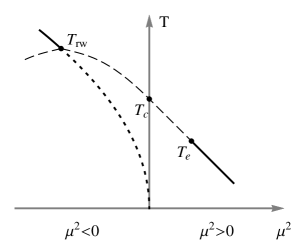
Figure 1: The phase diagram in the imaginary chemical potential plane. Solid lines indicate the first order phase transition and dotted lines cross-overs. The thin dashed lines represent either rapid crossovers or real transitions depending on the number of quark flavors and their mass.

To better understand this behavior recall that at high temperature the Polyakov loop is ordered and for $\mu=0$ the determinant favors the configurations with $\arg P\approx 0$. Using Eq. 4 this implies that for $\mu/T=\pm i2\pi/3$ the Polyakov loop will be aligned differently, i.e. $\arg P\approx\mp 2\pi/3$. The boundaries of these regions are the Roberge-Weiss lines $\mu/T\in\{i\pi,-i\pi/3,i\pi/3\}$. When we cross these lines at high temperatures the alignment of the Polyakov lines changes abruptly and we have a first order phase transition. At low temperatures the transition is smooth and we have a cross-over. The standard scenario is depicted in Fig. 1. The temperature where the Roberge-Weiss line changes from first order to cross-over is denoted with $T_{\text{rw}}$. The expectation is that the Roberge-Weiss transition point is connected with the (pseudo)critical transition point at zero density, $T_{c}$, which in turn is connected with the critical point at real imaginary chemical potential, $T_{e}$. Whether the lines connecting these points are phase transitions or cross-overs depends on the number of quarks in the system and their mass.

This is not the only logically possible scenario; alternative possibilities are depicted in Fig. 2: the (pseudo)critical line extending from zero density might terminate before intersecting the Roberge-Weiss line or intersect it at a temperature different than $T_{\text{rw}}$. It is then important to map out the phase diagram at imaginary chemical potential using direct simulations. The phase diagram at imaginary chemical potential was investigated for QCD with two degenerate quark flavors [2, 3, 4], three flavors [5], and four flavors [6, 7, 8] using staggered fermions. For $N_{f}=2,3$ staggered simulations use the standard determinant root technique and cross-checks with simulations using Wilson type fermions are required to remove any possible doubts. For $N_{f}=2$ this was done by Nagata and Nakamura [9]. In this talk we focus on the $N_{f}=3$ case.

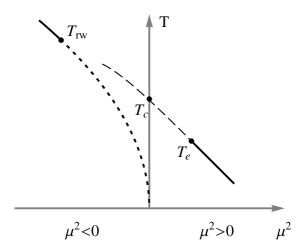
Figure 2: Alternative scenarios: the (pseudo)critical line extending from $\mu=0$ could terminate before touching the Roberge-Weiss line (left) or intersect it at a temperature different than $T_{\text{rw}}$.

2 Technical details

In this study we use gauge configurations generated using the Iwasaki gauge action and clover fermions. To determine the structure of the phase diagram we focus on the region $1.65\leq\beta\leq 1.73$ and $\mu_{I}/T\in[0,\pi/3]$. To reduce the number of ensembles needed in our investigation we used multi-histogram reweighting [10]. Since we plan to trace out the (pseudo)critical line extending from zero density into the imaginary chemical potential plane, we need to do a reweighting both in $\beta$ (temperature) and $\mu$. Schematically this can be achieved by introducing a reweighting factor $\alpha(U)$ via

$$\left\langle O(U)\right\rangle_{\beta,\mu}=\frac{\left\langle O(U)\alpha(U)\right\rangle_{\beta_{0},\mu_{0}}}{\left\langle\alpha(U)\right\rangle_{\beta_{0},\mu_{0}}}\,,$$ (9)

where

$$\alpha(U)\equiv e^{-(\beta-\beta_{0})S_{g}(U)}\frac{\det M(U,\mu)}{\det M(U,\mu_{0})}\,.$$ (10)

To compute the reweighting factor we need to compute a ratio of determinants. Our approach is to compute this ratio exactly using determinant compression method [11, 12]. The advantage of the compression method is that once the compressed matrix is diagonalized, we can compute the determinant for arbitrary values of the chemical potential as long as the other parameters are kept fixed. Thus, to facilitate this calculation we need to fix the value of the bare mass parameter $\kappa$ and the clover term $c_{\text{sw}}$. One of the goals for our study is to compare the reweighting results to results derived in canonical simulations [13]. We use the values that correspond to $T=0.87T_{c}$ in our $N_{f}=3$ study [14], $\kappa=0.13825$ and $c_{\text{sw}}=1.89374$. This corresponds to a pion mass of $m_{\pi}\approx 750\mathop{\hbox{MeV}}$.

In Fig. 3 we show the distribution of the Polyakov loops and the positions in the phase diagrams for the ensembles used in this study. Each ensemble has about $20,000$ configurations of size $6^{3}\times 4$. Note that the Polyakov loop prefers the real sector except for the ensembles generated at $\mu_{I}/T=\pi/3$. This is the Roberge-Weiss line and the $Z(2)$ symmetry is apparent. Note also that for $\beta=1.73$ the distribution of the Polyakov loops is bimodal indicating that the symmetry is spontaneously broken, whereas for lower temperatures the Polykov loops follow a unimodal distribution signaling a restoration of the symmetry.

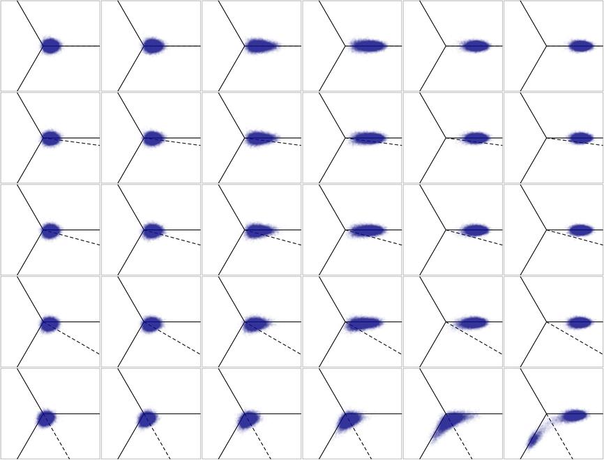
Figure 3: Left: Polyakov loop distribution for $\mu_{I}/T=0$, $\pi/24$, $\pi/12$, $\pi/6$, and $\pi/3$ (top to bottom) and $\beta=1.65$, $1.67$, $1.69$, $1.70$, $1.71$, and $1.73$ (left to right). The dashed line in each plot indicates the direction of $e^{-i\mu_{I}/T}$ in the complex plane. Right: the parameters of the generated ensembles and the (pseudo)critical curve as determined from this study.

3 Numerical results

To map out the phase diagram we determine the (pseudo)critical line extending from $\mu=0$ and the transition point on the Roberge-Weiss line. The first task can be accomplished by monitoring the Polyakov line magnitude as we increase the temperature for fixed $\mu_{I}/T$. In the right panel of Fig. 4 we show that Polyakov loop curves for $\mu_{I}/T=0$, $\pi/6$, $\pi/4$, and $\pi/3$. Note that the transition moves to higher temperature as we increase the imaginary chemical potential. To better pinpoint the transition point we determine the Polyakov loop susceptibility and locate the transition temperature at the point where the susceptibility reaches its maximal value. This is indicated in the lower figure from the right panel of Fig. 4. Using reweighting we can trace the transition temperature as a function of $\mu_{I}$. The results are presented in the left panel of Fig. 4. The curve is well described by the following function:

$$\beta_{c}\left(\frac{\mu_{I}}{T}\right)=c_{0}+c_{2}\left(\frac{\mu_{I}}{T}\right)^{2}+c_{4}\left(\frac{\mu_{I}}{T}\right)^{4}\,,$$ (11)

with $c_{0}=1.69658(3)$, $c_{2}=0.02014(6)$, and $c_{4}=0.00040(6)$.

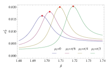
Figure 4: Left: the (pseudo)critical temperature as a function of imaginary chemical potential. Right: Absolute value of the Polyakov loop as a function of temperature for fixed $\mu_{I}/T$ (top) and its susceptibility (bottom).

The next task is to compute the transition temperature along the Roberge-Weiss line $\mu_{I}/T=\pi/3$. At high temperatures the Polyakov loop is expected to oscillate between $\arg(P)=0$ and $\arg(P)=-2\pi/3$ sectors and generate a bimodal distribution. As we lower the temperature the two peaks should get closer and eventually merge into one. This is exactly the situation we observe in the bottom panel of Fig. 5 where the probability distribution of $\varphi(U)=\mathop{\hbox{Im}}(P(U)\times e^{i\pi/3})$ is plotted for a set of increasing temperatures. To determine the location of the transition point more precisely we compute the Binder cumulant for this quantity:

$$b_{4}(\varphi)=\frac{\left\langle\varphi^{4}\right\rangle}{\left\langle\varphi^{2}\right\rangle^{2}}\,.$$ (12)

The Binder cumulant value is expected to be $3$, $1$, $1.604$, and $1.5$ for cross-overs, first-order transitions, second order in the $3$D Ising universality class, and triple point respectively. In the standard scenario, the expectation is that the Binder cumulant curve as a function of temperature will assume either the value of $1.604$ or $1.5$ as we intersect with the (pseudo)critical curve at $\beta_{c}(\pi/3)$. As we can see from Fig. 5 this expectation is close to what we observe. However, if we look closely we find that the intersection point is not very close to neither of these values. Since the statistical errors are quite small –they are comparable with the thickness of the line in Fig. 5– this must be a finite volume effect. Larger volume simulations are required to establish the exact nature of the transition and whether the (pseudo)critical line intersects the Roberge-Weiss line at the same temperature.

To conclude, we analyzed the phase diagram of $N_{f}=3$ QCD at a pion mass of $m_{\pi}=760\mathop{\hbox{MeV}}$. Our results are consistent with the Roberge-Weiss first order phase transition terminating at a point close to the (pseudo)critical curve. In this study we only used one lattice volume, $6^{3}\times 4$, and we cannot yet distinguish between a second order transition or a triple point. We plan to generate ensembles at larger volume and use finite size scaling to answer these questions.

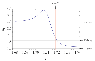
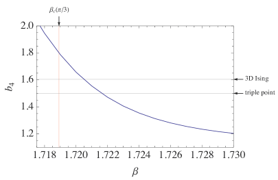
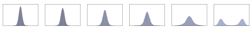
Figure 5: Top: the Binder cumulant for the phase of the Polyakov loop along the line $\mu_{I}/T=\pi/3$ (left) and a detailed look at the plot in the vicinity of $T_{\text{rw}}$ (right). We indicated on the graph the intersection between the (pseudo)critical line and Roberge-Weiss line, $\beta_{c}=\beta_{c}(\pi/3)$ and the expected values of the Binder cumulant for cross-over, first order, second order (3D Ising universality class) and triple point. Bottom: the distribution of the Polyakov phase as measured on the ensembles generated on the Roberge-Weiss line in order of increasing temperature from left to right.

Acknowledgments: The computational resources for this project were provided in part by the George Washington University IMPACT initiative and in part by the $\chi$QCD collaboration. This work is supported in part by the NSF CAREER grant PHY-1151648.

References

- [1] A. Roberge and N. Weiss, Gauge theories with imaginary chemical potential and the phases of QCD, Nucl. Phys. B275 (1986) 734.
- [2] P. de Forcrand and O. Philipsen, The QCD phase diagram for small densities from imaginary chemical potential, Nucl. Phys. B642 (2002) 290–306, [hep-lat/0205016].
- [3] M. D’Elia and F. Sanfilippo, The Order of the Roberge-Weiss endpoint (finite size transition) in QCD, Phys.Rev. D80 (2009) 111501, [arXiv:0909.0254].
- [4] M. D’Elia and F. Sanfilippo, Thermodynamics of two flavor QCD from imaginary chemical potentials, Phys.Rev. D80 (2009) 014502, [arXiv:0904.1400].
- [5] P. de Forcrand and O. Philipsen, Constraining the QCD phase diagram by tricritical lines at imaginary chemical potential, Phys.Rev.Lett. 105 (2010) 152001, [arXiv:1004.3144].
- [6] M. D’Elia and M.-P. Lombardo, Finite density QCD via imaginary chemical potential, Phys. Rev. D67 (2003) 014505, [hep-lat/0209146].
- [7] M. D’Elia and M. P. Lombardo, QCD thermodynamics from an imaginary : Results on the four flavor lattice model, Phys.Rev. D70 (2004) 074509, [hep-lat/0406012].
- [8] M. D’Elia, F. Di Renzo, and M. P. Lombardo, The strongly interacting quark gluon plasma, and the critical behaviour of QCD at imaginary , Phys.Rev. D76 (2007) 114509, [arXiv:0705.3814].
- [9] K. Nagata and A. Nakamura, Imaginary Chemical Potential Approach for the Pseudo-Critical Line in the QCD Phase Diagram with Clover-Improved Wilson Fermions, Phys.Rev. D83 (2011) 114507, [arXiv:1104.2142].
- [10] A. M. Ferrenberg and R. H. Swendsen, Optimized Monte Carlo analysis, Phys. Rev. Lett. 63 (1989) 1195–1198.
- [11] A. Alexandru and U. Wenger, QCD at non-zero density and canonical partition functions with Wilson fermions, Phys.Rev. D83 (2011) 034502, [arXiv:1009.2197].
- [12] K. Nagata and A. Nakamura, Wilson Fermion Determinant in Lattice QCD, Phys.Rev. D82 (2010) 094027, [arXiv:1009.2149].
- [13] A. Alexandru, M. Faber, I. Horváth, and K.-F. Liu, Lattice QCD at finite density via a new canonical approach, Phys.Rev. D72 (2005) 114513, [hep-lat/0507020].
- [14] A. Li, A. Alexandru, and K.-F. Liu, Critical point of QCD from lattice simulations in the canonical ensemble, Phys. Rev. D84 (2011) 071503, [arXiv:1103.3045].