Composite Channel Estimation
in Massive MIMO Systems

Abstract

We consider a multiuser (MU) multiple-input multiple-output (MIMO) time-division duplexing (TDD) system in which the base station (BS) is equipped with a large number of antennas for communicating with single-antenna mobile users. In such a system the BS has to estimate the channel state information (CSI) that includes large-scale fading coefficients (LSFCs) and small-scale fading coefficients (SSFCs) by uplink pilots. Although information about the former FCs are indispensable in a MU-MIMO or distributed MIMO system, they are usually ignored or assumed perfectly known when treating the MIMO CSI estimation problem. We take advantage of the large spatial samples of a massive MIMO BS to derive accurate LSFC estimates in the absence of SSFC information. With estimated LSFCs, SSFCs are then obtained using a rank-reduced (RR) channel model which in essence transforms the channel vector into a lower dimension representation.

We analyze the mean squared error (MSE) performance of the proposed composite channel estimator and prove that the separable angle of arrival (AoA) information provided by the RR model is beneficial for enhancing the estimator’s performance, especially when the angle spread of the uplink signal is not too large.

I Introduction

A cellular mobile network in which each base station (BS) is equipped with an $M$-antenna array, is referred to as a large-scale multiple-input, multiple-output (MIMO) system or a massive MIMO system for short if $M\gg 1$ and $M\gg K$, where $K$ is the number of active user antennas within its serving area. A massive MIMO system has the potentiality of achieving transmission rate much higher than those offered by current cellular systems with enhanced reliability and drastically improved power efficiency. It takes advantage of the so-called channel-hardening effect [1] which implies that the channel vectors seen by different users tend to be mutually orthogonal and frequency-independent [2]. As a result, linear receiver is almost optimal in the uplink and simple multiuser (MU) precoder are sufficient to guarantee satisfactory downlink performance. Although most investigation consider the co-located BS antenna array scenario [1], the use of a more general setting of massive distributed antennas has been suggested recently [3].

The Kronecker model [4], which assumes separable transmit and receive spatial statistics, is often used in the study of massive MIMO systems [5]. The spatial channel model (SCM) [6], which is adopted as the 3GPP standard, degenerates to the Kronecker model [7] when the number of subpaths approaches infinity. This model also implies that the distributions of angle of arrival (AoA) and angle of departure (AoD) are independent. In general such an assumption is valid if the antenna number is small and large cellular system is in question. But if one side of a MIMO link consists of multiple single-antenna terminals, only the spatial correlation of the array side needs to be taken into account and thus the reduced Kronecker model and other spatial correlated channel models become equivalent. Throughout this paper our investigation focuses on this practical scenario, i.e., we consider a massive MIMO system where $K$ is equal to the number of active mobile users.

We assume that the mobile users transmit orthogonal uplink pilots for the serving BS to estimate channel state information (CSI) that includes both small-scale fading coefficients (SSFCs) and large-scale fading coefficients (LSFCs). Besides data detection, CSI is needed for a variety of link adaptation applications such as precoder, modulation and coding scheme selection. The LSFCs, which summarize the pathloss and shadowing effect, are proportional to the average received signal strength (RSS) and are useful in power control, location estimation, hand-over protocol and other applications. While most existing works focus on the estimation of the channel matrix which ignores the LSFC [8, 9], it is desirable to know SSFCs and LSFCs separately. LSFCs are long-term statistics whose estimation is often more time-consuming than SSFCs estimation. Conventional MIMO CSI estimators usually assume perfect LSFC information and deal solely with SSFCs [3, 10, 11]. For co-located MIMO systems, it is reasonable to assume that the corresponding LSFCs remain constant across all spatial subchannels and the SSFC estimation can sometime be obtained without the LSFC information. Such an assumption is no longer valid in a multiuser MIMO (MU-MIMO) system where the user-BS distances spread over a large range and SSFCs cannot be derived without the knowledge of LSFCs.

The estimation of LSFC has been largely neglected, assuming somehow perfectly known prior to SSFC estimation. When one needs to obtain a joint LSFC and SSFC estimate, the minimum mean square error (MMSE) or least-squares (LS) criterion is not directly applicable. The expectation-maximization (EM) approach is a feasible alternate [12, Ch. 7] but it requires high computational complexity and cannot guarantee convergence. We propose an efficient algorithm for estimating LSFCs with no aid of SSFCs by taking advantage of the channel hardening effect and large spatial samples available to a massive MIMO BS. Our LSFC estimator is of low computational complexity, requires relatively small training overhead, and yields performance far superior to that of an EM-based estimator. Our analysis shows that it is unbiased and asymptotically optimal.

Estimation of SSFCs, on the other hand, is more difficult as the associated spatial correlation is not as high as that among LSFCs. Nevertheless, given an accurate LSFC estimator, we manage to derive a reliable SSFC estimator which exploits the spatial correlation induced channel rank reduction and calls for estimation of much less channel parameters than that required by conventional method [9] when the angle spread (AS) of the uplink signals is small. The proposed SSFC estimator provides excellent performance and offer additional information about the average AoA which is very useful in designing a downlink precoder.

The rest of this paper is organized as follows. In Section II, we describe a massive MU-MIMO channel model that takes into account spatial correlations and large-scale fading. In Section III, a novel uplink-pilot-based LSFC estimator is proposed and in Section IV, we devise an SSFC estimator by using the estimated LSFCs. Simulation results are presented in Section V to validate the superiority of our rank determination algorithm and CSI estimators in massive MU-MIMO systems. We summarize the main contributions in Section VI.

Notation: $(\cdot)^{T},(\cdot)^{H}$, and $(\cdot)^{*}$ represent the transpose, conjugate transpose, and conjugate of the enclosed items, respectively. $\mathrm{vec}(\cdot)$ is the operator that forms one tall vector by stacking columns of the enclosed matrix, whereas $\mathrm{Diag}(\cdot)$ translates a vector into a diagonal matrix with the vector entries being the diagonal terms. While $\mathbb{E}\{\cdot\}$, $\|\cdot\|$, $\|\cdot\|_{2}$, and $\|\cdot\|_{F}$ denote the expectation, vector $\ell_{2}$-norm, matrix spectral norm, and Frobenius norm of the enclosed items, respectively, $\otimes$ and $\odot$ respectively denote the Kronecker and Hadamard product operator. Denote by $\mathbf{I}_{L}$, $\mathbf{1}_{L}$, and $\mathbf{0}_{L}$ respectively the $L\times L$ identity matrix and $L$-dimensional all-one and all-zero column vectors, whereas $\mathbf{1}_{L\times S}$, and $\mathbf{0}_{L\times S}$ are the matrix counterparts of the latter two. $\mathbf{e}_{i}$ and $\mathbf{E}_{ij}$ are all-zero vector and matrix except for their $i$th and $(i,j)$th element being $1$, respectively.

II System Model

Consider a single-cell massive MU-MIMO system having an $M$-antenna BS and $K$ single-antenna mobile stations (MSs), where $M\gg K$. For a muti-cell system, pilot contamination [13] may become a serious design concern in the worst case when the same pilot sequences (i.e., the same pilot symbols are placed at the same time-frequency locations) happen to be used simultaneously in several neighboring cells and are perfectly synchronized in both carrier and time. In practice, there are frequency, phase and timing offsets between any pair of pilot signals and the number of orthogonal pilots is often sufficient to serve mobile users in multiple cells. Moreover, neighboring cells may use the same pilot sequence but the pilot symbols are located in non-overlapping time-frequency units [14], hence a pilot sequence is more likely be interfered by uncorrelated asynchronous data sequences whose impact is not as serious as the worst case and can be mitigated by proper inter-cell coordination, frequency planning and some interference suppression techniques [15]. We will, however, focus on the single-cell narrowband scenario throughout this paper.

We assume a narrowband communication environment in which a transmitted signal suffers from both large- and small-scale fading. The $K$ MS-BS link ranges are denoted by $d_{k}$ and each uplink packet place its pilot of length $T$ at the same time-frequency locations so that, without loss of generality, the corresponding received samples, arranged in matrix form, ${\bf Y}=[y_{ij}]$ at the BS can be expressed as

$$\mathbf{Y}=\sum_{k=1}^{K}\sqrt{\beta_{k}}\mathbf{h}_{k}\mathbf{p}_{k}^{H}+\mathbf{N}=\mathbf{H}\mathbf{D}_{\boldsymbol{\beta}}^{\frac{1}{2}}\mathbf{P}+\mathbf{N}$$ (1)

where $\mathbf{H}=[\mathbf{h}_{1},\cdots,\mathbf{h}_{K}]\in\mathbb{C}^{M\times K}$ and $\mathbf{D}_{\boldsymbol{\beta}}=\text{Diag}({\boldsymbol{\beta}})$ contain respectively the SSFCs and LSFCs that characterize the $K$ uplink channels, and $\mathbf{N}=[n_{ij}]$ is the white Gaussian noise matrix with independent identically distributed (i.i.d.) elements, $n_{ij}\sim\mathcal{CN}(0,1)$. Each element of the vector $\mathbf{\beta}=[\beta_{1},\cdots,\beta_{K}]^{T}$, $\beta_{k}={s_{k}}d_{k}^{-\alpha}$, is the product of the random variable $s_{k}$ representing the shadowing effect and the path loss $d_{k}^{\alpha}$, $\alpha>2$. $s_{k}$ are i.i.d. log-normal random variables, i.e., $10\log_{10}(s_{k})\sim\mathcal{N}(0,\sigma_{s}^{2})$. The $K\times T$ matrix $\mathbf{P}=\left[\mathbf{p}_{1},\cdots,\mathbf{p}_{K}\right]^{H}$, where $T\geq K$, consists of orthogonal uplink pilot vector $\mathbf{p}_{k}$. The optimality of using orthogonal pilots has been shown in [9].

It is reasonable to assume that the mobile users are relatively far apart (with respect to the wavelength) so that the $k$th uplink SSFC vector is independent of the $\ell$th vector, $\forall\ell\neq k$, and can be represented by

$$\mathbf{h}_{k}=\mathbf{\Phi}_{k}^{\frac{1}{2}}\tilde{\mathbf{h}}_{k},$$ (2)

where $\mathbf{\Phi}_{k}$ is the spatial correlation matrix at the BS side with respect to the $k$th user and $\tilde{\mathbf{h}}_{k}\sim\mathcal{CN}(\mathbf{0}_{M},\mathbf{I}_{M})$. We assume that $\tilde{\mathbf{h}}_{k}$’s are i.i.d. and the SSFC $\mathbf{H}$ remains constant during a pilot sequence period, i.e., the channel’s coherence time is greater than $T$, while the LSFC $\boldsymbol{\beta}$ varies much slower.

III Large-Scale Fading Coefficient Estimation

Unlike previous works on MIMO channel matrix estimation which either ignore LSFCs [8, 9] or assume perfect known LSFCs [3, 10, 11], we try to estimate $\mathbf{H}$ and $\mathbf{D}_{\boldsymbol{\beta}}$ jointly. We first introduce an efficient LSFC estimator without SSFCs information in this section. We treat separately channels with and without spatial correlation at the BS side and show that both cases lead to same estimators when the BS is equipped with a large-scale linear antenna array.

III-A Uncorrelated BS Antennas

We first consider the case when the BS antenna spacings are large enough that the spatial mode correlation is negligible. A statistic which is a function of the received sample matrix $\mathbf{Y}$ and LSFCs but is asymptotically independent of the SSFCs is derivable from the following property [16, Ch. 3].

Lemma 1

Let $\mathbf{p},\mathbf{q}\in\mathbb{C}^{M\times 1}$ be two independent $M$-dimensional complex random vectors with elements i.i.d. as $\mathcal{CN}(0,1)$. Then by the law of large number

$$\frac{1}{M}\mathbf{p}^{H}\mathbf{p}\stackrel{{\scriptstyle a.s.}}{{\longrightarrow}}1~{}~{}\text{and}~{}~{}\frac{1}{M}\mathbf{p}^{H}\mathbf{q}\stackrel{{\scriptstyle a.s.}}{{\longrightarrow}}0~{}\text{ as }~{}M\rightarrow\infty,$$

where $\stackrel{{\scriptstyle a.s.}}{{\longrightarrow}}$ denotes almost surely convergence.

For a massive MIMO system with $M\gg T\geq K$, we have, as $M\rightarrow\infty$, $\frac{1}{M}\mathbf{H}^{H}\mathbf{H}\stackrel{{\scriptstyle a.s.}}{{\longrightarrow}}\mathbf{I}_{K}$, $\frac{1}{M}\mathbf{N}^{H}\mathbf{N}\stackrel{{\scriptstyle a.s.}}{{\longrightarrow}}\mathbf{I}_{T}$, $\frac{1}{M}\mathbf{H}^{H}\mathbf{N}\stackrel{{\scriptstyle a.s.}}{{\longrightarrow}}\mathbf{0}_{K\times T}$, and thus

$$\frac{1}{M}\mathbf{Y}^{H}\mathbf{Y}-\mathbf{I}_{T} = \mathbf{P}^{H}\mathbf{D}_{\boldsymbol{\beta}}\mathbf{P}+\frac{1}{M}\mathbf{N}^{H}\mathbf{N}-\mathbf{I}_{T}$$ (3)

$$+\>\mathbf{P}^{H}\mathbf{D}_{\boldsymbol{\beta}}^{\frac{1}{2}}\left(\frac{1}{M}\mathbf{H}^{H}\mathbf{H}-\mathbf{I}_{K}\right)\mathbf{D}_{\boldsymbol{\beta}}^{\frac{1}{2}}\mathbf{P}~{}~{}~{}~{}~{}$$

$$+\>\frac{2}{M}\mathfrak{R}\left\{\mathbf{P}^{H}\mathbf{D}_{\boldsymbol{\beta}}^{\frac{1}{2}}\mathbf{H}^{H}\mathbf{N}\right\}$$

$$\stackrel{{\scriptstyle a.s.}}{{\longrightarrow}} \mathbf{P}^{H}\mathbf{D}_{\boldsymbol{\beta}}\mathbf{P}$$

(3) indicates that the additive noise effect is reduced and the estimation of LSFCs can be decoupled from that of the SSFCs. Using the identity, $\mathrm{vec}(\mathbf{A}\cdot\mathrm{Diag}(\mathbf{c})\cdot\mathbf{F})=\left((\mathbf{1}_{S}\otimes\mathbf{A})\odot(\mathbf{F}^{T}\otimes\mathbf{1}_{T})\right)\mathbf{c}$ with $\mathbf{A}\in\mathbb{C}^{T\times K}$, $\mathbf{F}\in\mathbb{C}^{K\times S}$, and $\mathbf{c}\in\mathbb{C}^{K\times 1}$, we simplify (3) as

$$\mathrm{vec}\left(\frac{1}{M}\mathbf{Y}^{H}\mathbf{Y}-\mathbf{I}_{T}\right)\stackrel{{\scriptstyle a.s.}}{{\longrightarrow}}\left(\left(\mathbf{1}_{T}\otimes\mathbf{P}^{H}\right)\odot\left(\mathbf{P}^{T}\otimes\mathbf{1}_{T}\right)\right)\boldsymbol{\beta}.$$

This equation suggests that we solve the following unconstrained convex problem

$$\underset{\boldsymbol{\beta}}{\min} \Bigg{\|}\mathrm{vec}\left(\frac{1}{M}\mathbf{Y}^{H}\mathbf{Y}-\mathbf{I}_{T}\right)$$

$$\hskip 70.0001pt-\left(\left(\mathbf{1}_{T}\otimes\mathbf{P}^{H}\right)\odot\left(\mathbf{P}^{T}\otimes\mathbf{1}_{T}\right)\right)\boldsymbol{\beta}\Bigg{\|}^{2},$$

to obtain the LSFC estimate

$$\hat{\boldsymbol{\beta}} = \mathrm{Diag}\left({\|\mathbf{p}_{1}\|^{-4}},\cdots,{\|\mathbf{p}_{K}\|^{-4}}\right)$$ (4)

$$~{}\cdot\left((\mathbf{1}_{T}^{T}\otimes\mathbf{P})\odot(\mathbf{P}^{*}\otimes\mathbf{1}_{T}^{T})\right)\mathrm{vec}\left(\frac{1}{M}\mathbf{Y}^{H}\mathbf{Y}-\mathbf{I}_{T}\right).~{}~{}~{}$$

This LSFC estimator is of low complexity as no matrix inversion is needed when orthogonal pilots are used and does not require any knowledge of SSFCs. Furthermore, the configuration of massive MIMO makes the estimator robust against noise, which is verified numerically later in Section V.

III-B Correlated BS Antennas

In practice, the spatial correlations are nonzero and $\mathbf{Y}$ is of the form

$$\mathbf{Y}=\tilde{\mathbf{\Phi}}\small{\left[\begin{array}[]{ccc}\tilde{\mathbf{h}}_{1}&\cdots&0\\ \vdots&\ddots&\vdots\\ 0&\cdots&\tilde{\mathbf{h}}_{K}\end{array}\right]}\mathbf{D}_{\boldsymbol{\beta}}^{\frac{1}{2}}\mathbf{P}+\mathbf{N}\stackrel{{\scriptstyle def}}{{=}}\tilde{\mathbf{\Phi}}\tilde{\mathbf{H}}\mathbf{D}_{\boldsymbol{\beta}}^{\frac{1}{2}}\mathbf{P}+\mathbf{N}$$ (8)

where $\tilde{\mathbf{\Phi}}=[\mathbf{\Phi}_{1}^{\frac{1}{2}},\cdots,\mathbf{\Phi}_{K}^{\frac{1}{2}}]$. Following [5, 17], we assume that the following is always satisfied:

Assumption 1

The spatial correlation at BS antennas seen by a user satisfies

$$\underset{{M\rightarrow\infty}}{\limsup}\|\mathbf{\Phi}_{k}^{\frac{1}{2}}\|_{2}<\infty,~{}~{}\forall k;$$

or equivalently,

$$\underset{{M\rightarrow\infty}}{\limsup}\|\mathbf{\Phi}_{k}\|_{2}<\infty,~{}~{}\forall k.$$

Therefore, (3) becomes

$$\frac{1}{M}\mathbf{Y}^{H}\mathbf{Y}-\mathbf{I}_{T} \stackrel{{\scriptstyle a.s.}}{{\longrightarrow}} \mathbf{P}^{H}\mathbf{D}_{\boldsymbol{\beta}}\mathbf{P}+\frac{2}{M}\mathfrak{R}\left\{\mathbf{P}^{H}\mathbf{D}_{\boldsymbol{\beta}}^{\frac{1}{2}}\tilde{\mathbf{H}}^{H}\tilde{\mathbf{\Phi}}^{H}\mathbf{N}\right\}$$

$$+\>\mathbf{P}^{H}\mathbf{D}_{\boldsymbol{\beta}}^{\frac{1}{2}}\left(\frac{1}{M}\tilde{\mathbf{H}}^{H}\tilde{\mathbf{\Phi}}^{H}\tilde{\mathbf{\Phi}}\tilde{\mathbf{H}}-\mathbf{I}_{K}\right)\mathbf{D}_{\boldsymbol{\beta}}^{\frac{1}{2}}\mathbf{P}~{}~{}~{}$$

$$\stackrel{{\scriptstyle def}}{{=}} \mathbf{P}^{H}\mathbf{D}_{\boldsymbol{\beta}}\mathbf{P}+\mathbf{N}^{\prime}$$

where $\mathbf{N}^{\prime}$ is zero-mean with seemingly non-diminishing variance due to the spatial correlation. Nonetheless, we proved in Appendix A that

Theorem 1

If $\underset{{M\rightarrow\infty}}{\limsup}\underset{{1\leq k\leq K}}{\sup}\|\mathbf{\Phi}_{k}^{\frac{1}{2}}\|_{2}<\infty$, then

$$\frac{1}{M}\tilde{\mathbf{H}}^{H}\tilde{\mathbf{\Phi}}^{H}\tilde{\mathbf{\Phi}}\tilde{\mathbf{H}} \stackrel{{\scriptstyle a.s.}}{{\longrightarrow}} \mathbf{I}_{K},$$ (9)

$$\frac{1}{M}\tilde{\mathbf{H}}^{H}\tilde{\mathbf{\Phi}}^{H}\mathbf{N} \stackrel{{\scriptstyle a.s.}}{{\longrightarrow}} \mathbf{0}_{K\times T}$$ (10)

as $M\rightarrow\infty$.

This theorem implies that although the nonzero spatial correlation does cause the increase of variance of $\mathbf{N}^{\prime}$, the channel hardening effect still exist and $\mathbf{N}^{\prime}$ is asymptotically diminishing provided that Assumption 1 holds. In this case, LS criterion also mandates the same estimator as (4). Several remarks are worth mentioning.

Remark 1

If $J$ consecutive coherence blocks in which the LSFCs remain constant are available, (4) can be rewritten as

$$\hat{\boldsymbol{\beta}} = \mathrm{Diag}\left({\|\mathbf{p}_{1}\|^{-4}},\cdots,{\|\mathbf{p}_{K}\|^{-4}}\right)\left[\left(\mathbf{1}_{T}^{T}\otimes\mathbf{P}\right)\odot\left(\mathbf{P}^{*}\otimes\mathbf{1}_{T}^{T}\right)\right]$$ (11)

$$~{}~{}~{}~{}~{}~{}~{}~{}~{}~{}~{}~{}~{}~{}~{}~{}~{}~{}~{}~{}~{}\cdot\mathrm{vec}\left(\frac{1}{MJ}\sum_{i=1}^{J}\mathbf{Y}_{i}^{H}\mathbf{Y}_{i}-\frac{1}{J}\mathbf{I}_{T}\right)$$

where $\mathbf{Y}_{i}$ is the $i$th received block. Moreover, the noise reduction effect becomes more evident as more received samples become available.

Remark 2

The proposed LSFC estimators (4) and (11) render element-wise expressions as

$$\hat{\beta}_{k} = \frac{\mathbf{p}_{k}^{H}\mathbf{Y}^{H}\mathbf{Y}\mathbf{p}_{k}-M\|\mathbf{p}_{k}\|^{2}}{M\|\mathbf{p}_{k}\|^{4}},~{}~{}\forall~{}k,$$ (12)

$$\hat{\beta}_{k} = \frac{\sum_{i=1}^{J}\mathbf{p}_{k}^{H}\mathbf{Y}^{H}_{i}\mathbf{Y}_{i}\mathbf{p}_{k}-MJ\|\mathbf{p}_{k}\|^{2}}{MJ\|\mathbf{p}_{k}\|^{4}},~{}~{}\forall~{}k.$$ (13)

III-C Performance Analysis

Since the mean of the LSFC estimator (12)

$$\mathbb{E}\left\{\hat{\beta}_{k}\right\} = \frac{\mathbf{p}_{k}^{H}(M\mathbf{P}^{H}\mathbf{D}_{\boldsymbol{\beta}}\mathbf{P}+M\mathbf{I}_{K})\mathbf{p}_{k}-M\|\mathbf{p}_{k}\|^{2}}{M\|\mathbf{p}_{k}\|^{4}}$$ (14)

$$= \frac{M\beta_{k}\|\mathbf{p}_{k}\|^{4}+M\|\mathbf{p}_{k}\|^{2}-M\|\mathbf{p}_{k}\|^{2}}{M\|\mathbf{p}_{k}\|^{4}}$$

$$= \beta_{k},~{}\forall~{}k,$$

the mean squared error (MSE) of $\hat{\beta}_{k}$

$$\mathrm{MSE}\left(\hat{\beta}_{k}\right)=\mathbb{E}\left\{\left|\hat{\beta}_{k}-\beta_{k}\right|^{2}\right\} = \mathrm{Var}\left\{\hat{\beta}_{k}\right\}.$$ (15)

Lemma 2

[16, Th. 3.4] Let $\mathbf{A}\in\mathbb{C}^{M\times M}$ and $\mathbf{p}$ and $\mathbf{q}$ be two vectors whose elements are i.i.d. as $\mathcal{CN}(0,1)$. If $\underset{{M\rightarrow\infty}}{\limsup}\|\mathbf{A}\|_{2}<\infty$, then

$$\mathbf{p}^{H}\mathbf{A}\mathbf{p}\stackrel{{\scriptstyle a.s.}}{{\longrightarrow}}\mathrm{tr}(\mathbf{A})~{}~{}\text{and}~{}~{}\frac{1}{M}\mathbf{p}^{H}\mathbf{A}\mathbf{q}\stackrel{{\scriptstyle a.s.}}{{\longrightarrow}}0~{}\text{ as }~{}M\rightarrow\infty.$$

Remark 3

Using [18, Lemma B.26], we can prove that the convergence rates in the aforementioned asymptotic formulae follow $\mathcal{O}({\|\mathbf{A}\|_{F}}/{M})$. More precisely,

$$\mathbb{E}\left\{\left|\frac{\mathbf{p}^{H}\mathbf{A}\mathbf{p}-\mathrm{tr}(\mathbf{A})}{M}\right|\right\} = \mathcal{O}({\|\mathbf{A}\|_{F}}/{M});$$ (16)

$$\mathbb{E}\left\{\left|\frac{\mathbf{p}^{H}\mathbf{A}\mathbf{q}}{M}\right|\right\} = \mathcal{O}({\|\mathbf{A}\|_{F}}/{M}).$$ (17)

By reformulating (12) as

$$\hat{\beta}_{k}=\beta_{k}+\underbrace{\frac{\mathbf{p}_{k}^{H}(\mathbf{N}^{H}\mathbf{N}-M\mathbf{I}_{K})\mathbf{p}_{k}}{M\|\mathbf{p}_{k}\|^{4}}}_{r_{1}}$$

$$+\underbrace{\frac{\beta_{k}(\mathbf{h}_{k}^{H}\mathbf{h}_{k}-M)}{M}}_{r_{2}} + \underbrace{\frac{\sqrt{\beta_{k}}\left(2\mathfrak{R}\left\{\mathbf{h}_{k}^{H}\mathbf{N}\mathbf{p}_{k}\right\}\right)}{M\|\mathbf{p}_{k}\|^{2}}}_{r_{3}},$$

and invoking Assumption 1, Lemmas 1 and 2, and the fact that $\mathbf{h}_{k}=\mathbf{\Phi}_{k}^{\frac{1}{2}}\tilde{\mathbf{h}}_{k}$, we conclude that $r_{1},r_{2},r_{3}\stackrel{{\scriptstyle a.s.}}{{\longrightarrow}}0$ as $M\rightarrow\infty$, and thus

$$\mathrm{Var}\left\{\hat{\beta}_{k}\right\} = \mathbb{E}\left\{|r_{1}+r_{2}+r_{3}|^{2}\right\}\stackrel{{\scriptstyle a.s.}}{{\longrightarrow}}0.$$ (18)

As $\beta_{k}$, $\mathbf{h}_{k}$, and $\mathbf{N}$ are uncorrelated, we have

$$\mathbb{E}\left\{|r_{1}+r_{2}+r_{3}|^{2}\right\}\approx\mathbb{E}\left\{|r_{1}|^{2}\right\}+\mathbb{E}\left\{|r_{2}|^{2}\right\}+\mathbb{E}\left\{|r_{3}|^{2}\right\}.$$

(19)

Since when pilot length $T=K$,

$$\mathbb{E}\left\{|r_{1}|^{2}\right\} = \|\mathbf{p}_{k}\|^{-8}\mathbb{E}\left\{\mathrm{tr}\left(\mathbf{p}_{k}\mathbf{p}_{k}^{H}\left(\frac{\mathbf{N}^{H}\mathbf{N}-M\mathbf{I}_{K}}{M}\right)\right)^{2}\right\}$$ (20)

$$\leq \|\mathbf{p}_{k}\|^{-8}\mathbb{E}\left\{\mathrm{tr}\left(\mathbf{p}_{k}\mathbf{p}_{k}^{H}\right)^{2}\mathrm{tr}\left(\frac{\mathbf{N}^{H}\mathbf{N}-M\mathbf{I}_{K}}{M}\right)^{2}\right\}$$

$$= K\|\mathbf{p}_{k}\|^{-4}\mathbb{E}\left\{\left(\frac{\mathbf{n}_{1}^{H}\mathbf{n}_{1}-M}{M}\right)^{2}\right\}$$

$$= \mathcal{O}\left(\frac{K}{\|\mathbf{p}_{k}\|^{4}}\frac{1}{M}\right)=\mathcal{O}\left(\frac{\beta_{k}^{2}}{T\cdot\mathrm{SNR}_{k}^{2}}\frac{1}{M}\right);$$

$$\mathbb{E}\left\{|r_{2}|^{2}\right\} = \beta_{k}^{2}\>\mathbb{E}\left\{\left|\frac{\tilde{\mathbf{h}}_{k}^{H}\mathbf{\Phi}_{k}\tilde{\mathbf{h}}_{k}-M}{M}\right|^{2}\right\}$$ (21)

$$= \mathcal{O}\left(\beta_{k}^{2}\frac{\|\mathbf{\Phi}_{k}\|_{F}^{2}}{M^{2}}\right)\gg\mathcal{O}\left(\beta_{k}^{2}\frac{1}{M}\right);$$

$$\mathbb{E}\left\{|r_{3}|^{2}\right\} = \frac{4\beta_{k}}{\|\mathbf{p}_{k}\|^{4}}\mathbb{E}\left\{\left|\frac{\mathfrak{R}\left\{\mathbf{h}_{k}^{H}\mathbf{N}\mathbf{p}_{k}\right\}}{M}\right|^{2}\right\}$$ (22)

$$\leq \frac{4\beta_{k}}{\|\mathbf{p}_{k}\|^{4}}\mathbb{E}\left\{\left|\frac{\mathbf{h}_{k}^{H}\mathbf{N}\mathbf{p}_{k}}{M}\right|^{2}\right\}\leq\frac{4\beta_{k}}{\|\mathbf{p}_{k}\|^{2}}\mathbb{E}\left\{\frac{\left\|\mathbf{N}^{H}\mathbf{h}_{k}\right\|^{2}}{M^{2}}\right\}$$

$$= \frac{4K\beta_{k}}{\|\mathbf{p}_{k}\|^{4}}\mathbb{E}\left\{\left|\frac{\mathbf{n}_{1}^{H}\mathbf{\Phi}_{k}^{\frac{1}{2}}\tilde{\mathbf{h}}_{k}}{M}\right|^{2}\right\}$$

$$= \frac{4K\beta_{k}}{\|\mathbf{p}_{k}\|^{2}}\mathcal{O}\left(\frac{\|\mathbf{\Phi}_{k}^{\frac{1}{2}}\|_{F}^{2}}{M^{2}}\right)=\mathcal{O}\left(\frac{4\beta_{k}^{2}}{\mathrm{SNR}_{k}}\frac{1}{M}\right),$$

where $\mathrm{SNR}_{k}\stackrel{{\scriptstyle def}}{{=}}{\beta_{k}\|\mathbf{p}_{k}\|^{2}}/{T}$, we obtain the following

Lemma 3

The convergence rate for the MSE of LSFC estimate $\hat{\beta}_{k}$ is dominated by the term $\mathbb{E}\left\{|r_{2}|^{2}\right\}$ when $T=K$.

Corollary 1

The LSFC estimators (4) and (11) approach the minimum mean-square error (MMSE) estimator with asymptotically diminishing MSE as $M\rightarrow\infty$.

Remark 4

As $\mathbb{E}\left\{|r_{2}|^{2}\right\}$ is the only term in (19) related to spatial correlation, for cases with finite $M$, the MSE-minimizing spatial correlation matrix $\mathbf{\Phi}_{k}^{\star}$ is the solution of

$$\min_{\mathbf{A}} ~{}~{}\mathbb{E}\left\{\left|\tilde{\mathbf{h}}_{k}^{H}\mathbf{A}\tilde{\mathbf{h}}_{k}\right|^{2}\right\}-\mathrm{tr}(\mathbf{A})$$

$$\mathrm{s.t.} ~{}~{}[\mathbf{A}]_{ii}=1,~{}\forall~{}i.$$ (23)

Following the method of Lagrange multiplier, we obtain $\mathbf{\Phi}_{k}^{\star}=\mathbf{I}_{M}$. The convexity of (23) implies that $\mathrm{Var}\{\hat{\beta}_{k}\}$ is an increasing function of $\|\mathbf{\Phi}_{k}-\mathbf{I}_{M}\|_{F}$, i.e., the MSE of the LSFC estimator decreases as the channel becomes less correlated; meanwhile, Lemma 3 guarantees the error convergence rate improvement.

Remark 5 (Finite $M$ scenario)

Low MSE, in the order of $10^{-5}$ to $10^{-4}$ if normalized by LSFCs’ variance, is obtainable with not-so-large BS antenna numbers (e.g., $50$). The above MSE performance analysis is validated via simulation in Section V.

IV Estimation of Small-Scale Fading Coefficients

Since the SSFC estimation scheme is valid for any user-BS link, for the sake of brevity, we omit the user index $k$ in the ensuing discussion.

IV-A Reduced-Rank Channel Modeling

In [19], two analytic correlated MIMO channel models were proposed. These models generalize and encompass as special cases, among others, the Kronecker [4, 20], virtual representation [21] and Weichselberger [22] models. They often admit flexible reduced-rank representations. Moreover, if the AS of the transmit signal is small, which, as reported in a recent measurement campaign [2], is the case when a large uniform linear array (ULA) is used at the BS, one of the models can provide AoA information. In other words, since the ASs from uplink users in a massive MIMO system are relatively small (say, less than $15^{\circ}$), the following rank-reduced (RR) model is easily derivable from [19]

Lemma 4 (RR representations)

The channel vector seen by $k$th user can be represented by

$$\mathbf{h}=\mathbf{Q}_{m}^{(\textrm{I})}\mathbf{c}^{(\textrm{I})}$$ (24)

or alternately by

$$\mathbf{h}=\mathbf{W}(\phi)\mathbf{Q}_{m}^{(\textrm{II})}\mathbf{c}^{(\textrm{II})}$$ (25)

where $\mathbf{Q}_{m}^{(\textrm{I})},\mathbf{Q}_{m}^{(\textrm{II})}\in\mathbb{C}^{M\times m}$ are predetermined basis (unitary) matrices and $\mathbf{c}^{(\textrm{I})},\mathbf{c}^{(\textrm{II})}\in\mathbb{C}^{m\times 1}$ are the transformed channel vectors with respect to bases $\mathbf{Q}_{m}^{(\textrm{I})}$ and $\mathbf{Q}_{m}^{(\textrm{II})}$ for the user $k$-BS link and $\mathbf{W}(\phi)$ is diagonal with unit magnitude entries. The two equalities hold only if $m=M$ and become approximations if $m<M$.

Remark 6

It was shown [19] that for an uniform linear array (ULA) with antenna spacing $\xi$ and incoming signal wavelength $\lambda$, if $[\mathbf{W}(\phi)]_{ii}=\exp\left(-j2\pi\frac{(i-1)\xi}{\lambda}\sin\phi\right)$, then $\phi$ can be interpreted as the mean AoA with respect to the ULA broadside when AS of ${\bf h}$ is assumed to be small. A direct implication is that the mean AoA (which is approximately equal to the incident angle of the strongest path) of each user link is extractable if the associated AS is small. (See Appendix C.)

Remark 7

The measurement reported in [2] verified that the AS for each MS-BS link is indeed relatively small when the BS is equipped with a large-scale linear array. Hence, a massive MIMO channel estimator based on the model (25) is capable of offering accurate mean AoA information [1] which can then be used by the BS to perform downlink beamforming.

Remark 8

(21) implies that for the user $k$ to BS link, we are interested in estimating the transformed vector $\mathbf{c}_{k}={\bf Q}^{H}_{m}\mathbf{W}^{H}(\phi_{k}){\bf h}_{k}$ which is obtained by realigning ${\bf h}_{k}$ and transform it into a new orthogonal coordinate. The best dimension reduction is obtained by setting ${\bf Q}_{m}$ as the one that consists of the eigenvectors associated with the largest $m$ eigenvalues of the expected Gram matrix $\mathbb{E}\left\{\mathbf{W}^{H}(\phi_{k}){\bf h}_{k}{\bf h}_{k}^{H}\mathbf{W}(\phi_{k})\right\}=\mathbf{W}^{H}(\phi_{k})\mathbb{E}\{{\bf h}_{k}{\bf h}_{k}^{H}\}\mathbf{W}(\phi_{k})=\mathbf{W}^{H}(\phi_{k})\Phi_{k}\mathbf{W}(\phi_{k})$.

Remark 9

The use of predetermined unitary matrices ${\bf Q}_{m}$ in both (24) and (25) avoids the estimation of the above correlation matrix $\mathbf{\Phi}_{k}$ and the ensuing eigen-decomposition for each $k$ to obtain the associated Karhunen-Loève transform (KLT) basis (eigen vectors). For large-scale ULAs, due to space limitation, the spatial correlation can be high and small $m$ is sufficient to capture the spatial variance of the SSFCs if an appropriate basis matrix is preselected. This is also validated via simulation in Section V. The advantages of (25) with respect to (24) are that the former can offer additional AoA information when AS is relatively small and because of the extra alignment operation $\mathbf{W}^{H}(\phi_{k})$, it makes the resulting Gram matrix closer to a real matrix.

IV-B Predetermined Basis for RR Channel Modeling

In addition, KLT basis is nonflexible in that it is channel-dependent and computationally expensive to obtain. Thus, prior to the SSFC estimation, eigen-decomposition and eigenvalue ordering must be performed to the spatial correlation matrix of $\mathbf{W}^{H}(\phi)\mathbf{h}$, which varies from user to user and can be accurately estimated only if sufficient observations are collected. As a result, it is unrealistic to apply KLT bases in the multiuser SSFC estimation. Our channel model (25) uses a predetermined signal-independent basis $\mathbf{Q}_{m}$ which requires far less complexity. Two candidate bases are of special interest to us for their proximity to the KLT basis.

IV-B1 Polynomial Basis [19]

As the BS antenna spatial correlation is often reasonably smooth, polynomial basis of dimension $m<M$ may be sufficient to track the channel variation. To construct an orthonormal discrete polynomial basis we perform standard QR decomposition $\mathbf{U}=\mathbf{Q}\mathbf{R}$, where $[\mathbf{U}]_{ij}=(i-1)^{j-1}$, $\forall i,j=1,\cdots,M$. Since the polynomial degree of each column of $\mathbf{Q}$ are arranged in an ascending order, the RR basis $\mathbf{Q}_{m}$ is obtained by keeping the first $m$ columns.

IV-B2 Type-$2$ Discrete Cosine Transform (DCT) Basis [25]

DCT, especially Type-$2$ DCT (DCT-$2$ or simply DCT), is a widely used for image coding for its excellent energy compaction capability [26, 25]. For a smooth finite-length sequence, its DCT is often energy-concentrated in lower-indexed coefficients. Hence the DCT basis matrix

$$[\mathbf{Q}_{m}]_{ij}={q}_{j}\cos\left(\frac{\pi(2i-1)(j-1)}{2M}\right),$$ (26)

for $1\leq i\leq M$ and $1\leq j\leq m$, where $1\leq m\leq M$ and

$$q_{j}=\left\{\begin{array}[]{ll}\sqrt{{1}/{M}},&j=1;\\ \sqrt{{2}/{M}},&j=2,\cdots,M.\end{array}\right.$$ (29)

is an excellent candidate RR basis for our channel estimation purpose. Some comments on the predetermined basis selection are provided in [23, 24].

Remark 10

As will be seen in the ensuing subsection, the proposed SSFC estimator can be realized by performing an inverse DCT or KLT on the received signal vector but the complexity of computing KLT and DCT are respectively $\mathcal{O}(M^{2})$ and $\mathcal{O}(M\log_{2}M)$. On the other hand, both polynomial basis and DCT basis do not need the spatial correlation information but DCT basis is computationally more efficient than the polynomial basis.

Remark 11

The fact that the energy compaction efficiency of DCT is near-optimal makes it the closest KLT approximation in the high correlation regime among the following unitary transforms: Walsh-Hadamard, Slant, Haar, and discrete Legendre transform, where the last one is equivalent to a polynomial-based transform and is slightly inferior to DCT in energy compaction capability.

The above claims have been verified in the context of image compression [23, 24]. In terms of RR MIMO channel representation, we show in Section V that, for the same modeling order $m$, the DCT basis does outperform the polynomial basis in MU SSFC estimation error regardless of the correlation level.

IV-C SSFC Estimation

We begin with the channel model (24) and denote by $\boldsymbol{\epsilon}^{(\textrm{I})}$ the modeling error. Let ${\gamma}=\sqrt{{\beta}}\|\mathbf{p}\|^{2}$ and assume for the moment that LSFCs are known. Then

$$\mathbf{Y}\mathbf{p} = {\sqrt{\beta}}\|\mathbf{p}\|^{2}\mathbf{h}+\mathbf{N}\mathbf{p}$$ (30)

$$= \gamma\left(\mathbf{Q}_{m}^{(\textrm{I})}\mathbf{c}^{(\textrm{I})}+\boldsymbol{\epsilon}^{(\textrm{I})}\right)+\mathbf{N}\mathbf{p}$$

which brings about the following LS problem

$$\underset{{\mathbf{c}}}{\min}~{}~{}\left\|\mathbf{Y}\mathbf{p}-\gamma\mathbf{Q}_{m}^{(\textrm{I})}\mathbf{c}^{(\textrm{I})}\right\|^{2}$$ (31)

The optimal solution can be shown as

$$\hat{\mathbf{c}}^{(\textrm{I})}=\frac{1}{\gamma}\left(\mathbf{Q}_{m}^{(\textrm{I})}\right)^{H}\mathbf{Y}\mathbf{p}.$$ (32)

Replacing $\gamma$ by $\hat{\gamma}=\hat{\beta}^{\frac{1}{2}}\|\mathbf{p}\|^{2}$ for the case when LSFCs have to be estimated, we have

$$\hat{\mathbf{h}}^{(\textrm{I})}=\mathbf{Q}_{m}^{(\textrm{I})}\hat{\mathbf{c}}^{(\textrm{I})}=\frac{1}{\gamma}\mathbf{Q}_{m}^{(\textrm{I})}\left(\mathbf{Q}_{m}^{(\textrm{I})}\right)^{H}\mathbf{Y}\mathbf{p}.$$ (33)

On the other hand, if (25) is the channel model and $\boldsymbol{\epsilon}^{(\textrm{II})}$ is the corresponding modeling error, then

$$\mathbf{Y}\mathbf{p} = {\sqrt{\beta}}\|\mathbf{p}\|^{2}\mathbf{h}+\mathbf{N}\mathbf{p}$$ (34)

$$= \gamma\left(\mathbf{W}(\phi)\mathbf{Q}_{m}^{(\textrm{II})}\mathbf{c}^{(\textrm{II})}+\boldsymbol{\epsilon}^{(\textrm{II})}\right)+\mathbf{N}\mathbf{p}$$

which suggests the LS formulation

$$\min_{\phi,\mathbf{c}} ~{}~{}\left\|\mathbf{Y}\mathbf{p}-\gamma\mathbf{W}(\phi)\mathbf{Q}_{m}^{(\textrm{II})}\mathbf{c}^{(\textrm{II})}\right\|^{2}$$

$$\mathrm{s.t.} ~{}~{}\mathbf{W}(\phi)={\mathrm{Diag}}\left(\omega_{1}(\phi),\cdots,\omega_{M}(\phi)\right),$$ (35)

$$~{}~{}~{}\omega_{i}(\phi)=\exp\left(-j2\pi\frac{(i-1)\xi}{\lambda}\sin\phi\right).$$

With $\mathbf{F}_{m}(\phi)\stackrel{{\scriptstyle def}}{{=}}\mathbf{W}(\phi)\mathbf{Q}_{m}^{(\textrm{II})}$ and $\mathbf{A}^{\dagger}\stackrel{{\scriptstyle def}}{{=}}(\mathbf{A}^{H}\mathbf{A})^{-1}\mathbf{A}^{H}$, the optimal solution to (IV-C) is given as

$$\hat{\phi} = \underset{\phi\in[-\frac{\pi}{2},\frac{\pi}{2}]}{\arg\max}~{}\mathbf{p}^{H}\mathbf{Y}^{H}\mathbf{F}_{m}(\phi)\mathbf{F}_{m}^{\dagger}(\phi)\mathbf{Y}\mathbf{p}$$ (36)

$$= \underset{\phi\in[-\frac{\pi}{2},\frac{\pi}{2}]}{\arg\max}~{}\left\|\left(\mathbf{W}(\phi)\mathbf{Q}_{m}^{(\textrm{II})}\right)^{H}\mathbf{Y}\mathbf{p}\right\|^{2}.$$

$$\hat{\mathbf{c}}^{(\textrm{II})} = \frac{1}{\gamma}\mathbf{F}_{m}^{\dagger}(\hat{\phi})\mathbf{Y}\mathbf{p}=\frac{1}{\gamma}\left(\mathbf{Q}_{m}^{(\textrm{II})}\right)^{H}\mathbf{W}^{H}(\hat{\phi})\mathbf{Y}\mathbf{p},$$ (37)

When the true LSFCs are not available we use their estimates, $\hat{\gamma}=\hat{\beta}^{\frac{1}{2}}\|\mathbf{p}\|^{2}$, and obtain the SSFCs estimate

$$\hat{\mathbf{h}}^{(\textrm{II})}=\mathbf{W}(\hat{\phi})\mathbf{Q}_{m}^{(\textrm{II})}\hat{\mathbf{c}}^{(\textrm{II})}.$$ (38)

Both (36) and (37) require no matrix inversion while $\hat{\phi}$ can be easily found by a simple line search.

IV-D Performance Analysis

Assuming perfect LSFC knowledge, (33) becomes

$$\hat{\mathbf{h}}^{(\textrm{I})} = \frac{1}{\gamma}\mathbf{Q}_{m}^{(\textrm{I})}\left(\mathbf{Q}_{m}^{(\textrm{I})}\right)^{H}(\gamma\mathbf{h}+\mathbf{N}\mathbf{p})\stackrel{{\scriptstyle def}}{{=}}\mathbb{E}\{\hat{\mathbf{h}}^{(\textrm{I})}\}+\boldsymbol{\nu}^{(\textrm{I})},~{}~{}$$ (39)

where $\boldsymbol{\nu}^{(\textrm{I})}=\frac{1}{\gamma}\mathbf{Q}_{m}^{(\textrm{I})}\left(\mathbf{Q}_{m}^{(\textrm{I})}\right)^{H}\mathbf{N}\mathbf{p}$, and with (37) substituting into it, (38) becomes

$$\hat{\mathbf{h}}^{(\textrm{II})} = \frac{1}{\gamma}\mathbf{W}(\hat{\phi})\mathbf{Q}_{m}^{(\textrm{II})}\left(\mathbf{Q}_{m}^{(\textrm{II})}\right)^{H}\mathbf{W}^{H}(\hat{\phi})\mathbf{Y}\mathbf{p}$$ (40)

$$= \frac{1}{\gamma}\mathbf{W}(\hat{\phi})\mathbf{Q}_{m}^{(\textrm{II})}\left(\mathbf{Q}_{m}^{(\textrm{II})}\right)^{H}\mathbf{W}^{H}(\hat{\phi})(\gamma\mathbf{h}+\mathbf{N}\mathbf{p})~{}~{}~{}~{}$$

$$\stackrel{{\scriptstyle def}}{{=}} \mathbb{E}\{\hat{\mathbf{h}}^{(\textrm{II})}\}+\boldsymbol{\nu}^{(\textrm{II})},$$

where $\boldsymbol{\nu}^{(\textrm{II})}=\frac{1}{\gamma}\mathbf{W}(\hat{\phi})\mathbf{Q}_{m}^{(\textrm{II})}\left(\mathbf{Q}_{m}^{(\textrm{II})}\right)^{H}\mathbf{W}^{H}(\hat{\phi})\mathbf{N}\mathbf{p}$. We denote by $\mathrm{MSE}_{m}(\cdot)$ the MSE of the enclosed SSFC estimate with modeling order $m$ and decompose it into

$$\mathrm{MSE}_{m}(\hat{\mathbf{h}}) = \mathbb{E}\left\{\left\|\hat{\mathbf{h}}-\mathbf{h}\right\|^{2}\right\}$$

$$= \underbrace{\mathbb{E}\left\{\left\|\hat{\mathbf{h}}-\mathbb{E}\{\hat{\mathbf{h}}\}\right\|^{2}\right\}}_{\stackrel{{\scriptstyle def}}{{=}}\mathrm{Var}\{{\hat{\mathbf{h}}}\}}+\underbrace{\mathbb{E}\left\{\left\|\mathbb{E}\{\hat{\mathbf{h}}\}-\mathbf{h}\right\|^{2}\right\}}_{\stackrel{{\scriptstyle def}}{{=}}b({\hat{\mathbf{h}}})}\vspace{-1.2em}$$

$\mathrm{Var}\{{\hat{\mathbf{h}}}\}$ and $b({\hat{\mathbf{h}}})$ represent respectively the variance and bias of estimator $\hat{\mathbf{h}}$. For these two error terms we prove in Appendix B that

Theorem 2

For SSFC estimators $\hat{\mathbf{h}}^{(\textrm{I})}$ and $\hat{\mathbf{h}}^{(\textrm{II})}$,

$$\mathrm{Var}\{\hat{\mathbf{h}}^{(\textrm{I})}\}=\mathrm{Var}\{\hat{\mathbf{h}}^{(\textrm{II})}\} = \frac{m}{\beta\|\mathbf{p}\|^{2}},$$

and

$$b(\hat{\mathbf{h}}^{(\textrm{I})}) = \mathrm{tr}\left(\mathbf{D}_{m}\left(\mathbf{Q}^{(\textrm{I})}\right)^{H}\mathbf{\Phi}\mathbf{Q}^{(\textrm{I})}\right)$$

$$b(\hat{\mathbf{h}}^{(\textrm{II})}) = \mathrm{tr}\left(\mathbf{D}_{m}\left(\mathbf{Q}^{(\textrm{II})}\right)^{H}\mathbf{W}^{H}(\hat{\phi})\mathbf{\Phi}\mathbf{W}(\hat{\phi})\mathbf{Q}^{(\textrm{II})}\right)$$

where $\mathbf{D}_{m}=\mathrm{Diag}\left(\left[\mathbf{0}_{1\times m}~{}\mathbf{1}_{1\times(M-m)}\right]^{T}\right)$.

Remark 12

If full-rank model, $m=M$, is used, then $\mathbf{Q}_{m}\mathbf{Q}_{m}^{H}=\mathbf{I}_{M}$. It is easy to check ${\bf D}_{m}={\bf 0}_{M}$ and to see from (33) and (38) that the proposed SSFC estimators $\hat{\mathbf{h}}^{(\textrm{I})}$ and $\hat{\mathbf{h}}_{k}^{(\textrm{II})}$ equivalent to the conventional unbiased LS estimator [9]

$$\hat{\mathbf{h}}=\frac{1}{\gamma}\mathbf{Y}\mathbf{p}.$$ (42)

V Simulation Results

In this section, we investigate the performance of the proposed estimators via simulation with a standardized channel model–SCM–whose spatial correlation at the BS is related to AoA distribution and antenna spacings [6]. In addition, the environment surrounding a user is of rich scattering with AoDs uniformly distributed in $[-\pi,\pi)$ making spatial correlation between MSs negligible. This setting accurately describes the environment where the BS with large-scale antenna array are mounted on an elevated tower or building. We assume that there are $8$ users located randomly in a circular cell of radius $R$ with their mean AoAs uniformly distributed within $[-60^{\circ},60^{\circ}]$. The other simulation parameters are listed in Table I. We define average received signal-to-noise power ratio as $\mathrm{SNR}\stackrel{{\scriptstyle def}}{{=}}\beta\|\mathbf{p}\|^{2}/T$ and normalized MSE (NMSE) as the MSE between the true and estimated vectors normalized by the former’s dimension and entry variance. Note that for LSFC estimation,

$$\mathrm{NMSE}(\hat{\beta}_{\textrm{dB}})\stackrel{{\scriptstyle def}}{{=}}\mathbb{E}\left\{\left(10\log{\hat{\beta}}/{\beta}\right)^{2}\right\}/\mathrm{Var}\{10\log\beta\}$$

instead of $\mathrm{NMSE}(\hat{\beta})$ is considered in this section.

TABLE I: Simulation parameters

Parameter	Value
Cell radius $R$	$100$ meters
Pathloss exponent $\alpha$	$3$
Shadowing standard deviation $\sigma_{s}$	$10$ dB
Number of BS antennas $M$	$100$
BS antenna spacing $\xi$	0.5$\lambda$
Number of MSs $K$	$8$
Number of path in SCM	$1$
Number of subpath in SCM	$20$

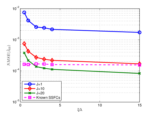
Figure 1: Effect of antenna spacing on the conventional LSFC estimator (with perfect SSFC knowledge) and proposed LSFC estimators using one or multiple blocks; $\mathrm{AS}=15^{\circ}$, $\mathrm{SNR}=10$ dB.

In Fig. 1 we compare the performance of the proposed LSFC estimators (4) and (11) with that of a conventional LS estimator [12, Ch. 8]

$$\widehat{\sqrt{\boldsymbol{\beta}}}=(\mathbf{A}^{H}\mathbf{A})^{-1}\mathbf{A}^{H}\mathrm{vec}(\mathbf{Y}),$$ (43)

where $\mathbf{A}=\left(\mathbf{1}_{T}\otimes\mathbf{H}\right)\odot\left(\mathbf{P}^{T}\otimes\mathbf{1}_{M}\right)$. As opposed to our proposal, the conventional estimator needs to know SSFCs beforehand, hence full knowledge of SSFCs is assumed for the latter. As can be seen, as antenna spacing increases, the channel decorrelates and thus the estimation error due to spatial correlation decreases; this verifies Theorem 1. Figure 1 also shows that our proposed estimator attains the performance of the conventional one (using one block) when channel correlation decreases to $0$ with $J=10$ training blocks and outperforms the conventional when $J=20$. This suggests that we can have good LSFC estimates even when the SSFCs are not available due to the advantage of the noise reduction effect that massive MIMO systems have offered.

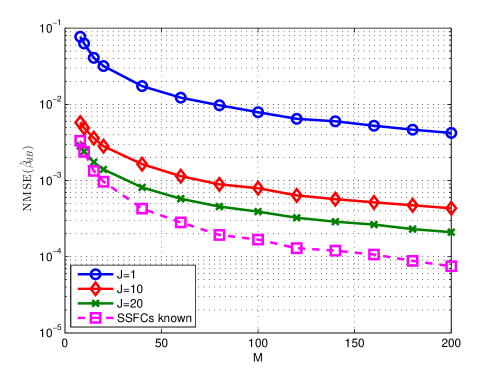
Figure 2: Large-system performance of the proposed LSFC estimators using one or more pilot blocks and that of the conventional estimator with perfect SSFC knowledge; $\mathrm{AS}=15^{\circ}$, $\mathrm{SNR}=10$ dB.

On the other hand, Fig. 2 illustrates the effect of massive antennas to the MSE. Owing to the fact that we have assumed perfect SSFC knowledge for the conventional LSFC estimator, MSE decreases with increasing sample amount as $M$ increases. Unlike the conventional, the amount of known information does not grow with $M$ for the proposed LSFC estimator. However, channel hardening effect becomes more serious and thus improves the estimator accuracy.

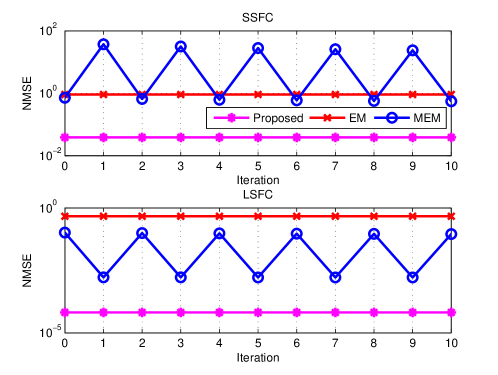
Figure 3: MSE performance of two EM-based joint LSFC/SSFC estimators versus their iteration numbers (which means initialization for value $0$); $\mathrm{AS}=7.2^{\circ}$, $\mathrm{SNR}=10$ dB. MSE of the proposed full-order SSFC and LSFC estimators is also plotted.

The performance of an EM-based joint LSFC and SSFC estimation is shown in Fig. 3. When the LSFC and SSFCs of an MS-BS link are all unknown and channel hardening effect in massive MIMO is disregarded, the coupling nature of the LSFC and SSFCs suggests EM algorithm be applied to derive their estimator. The EM-based joint LSFC and SSFC estimation is detailed as follows with $\sqrt{\boldsymbol{\beta}}\stackrel{{\scriptstyle def}}{{=}}[\sqrt{\beta_{1}},\cdots,\sqrt{\beta_{K}}]^{T}$:

1. (Initialization) Initialize $\widehat{\sqrt{\boldsymbol{\beta}}}=\mathbb{E}\{\sqrt{\boldsymbol{\beta}}\}$.

2. (Updating SSFC Estimates) Let $\hat{\boldsymbol{\beta}}=\left(\widehat{\sqrt{\boldsymbol{\beta}}}\right)^{2}$. Calculate

   $$\mathrm{vec}(\hat{\mathbf{H}})=\mathrm{Diag}\Big{(}(\mathbf{\Phi}_{1}+\|\mathbf{p}_{1}\|^{2}\hat{\beta}_{1}\mathbf{I}_{M})^{-1},\cdots,~{}~{}$$

   $$(\mathbf{\Phi}_{K}+\|\mathbf{p}_{K}\|^{2}\hat{\beta}_{K}\mathbf{I}_{M})^{-1}\Big{)}$$

   $$\cdot\left(\mathbf{D}_{\hat{\boldsymbol{\beta}}}^{\frac{1}{2}}\mathbf{P}^{\star}\otimes\mathbf{I}_{M}\right) \mathrm{vec}(\mathbf{Y}).~{}~{}~{}$$

3. (Updating LSFC Estimates) Calculate

   $$\widehat{\sqrt{\boldsymbol{\beta}}}=\mathbb{E}\left\{\sqrt{\boldsymbol{\beta}}\right\} + \left(\mathbf{C}^{-1}+\mathbf{A}^{H}\mathbf{A}\right)^{-1}$$

   $$~{}\cdot\mathbf{A}^{H}\left(\mathrm{vec}(\mathbf{Y})-\mathbf{A}\>\mathbb{E}\left\{\sqrt{\boldsymbol{\beta}}\right\}\right)$$

   where $\mathbf{A}=\left(\mathbf{1}_{T}\otimes\hat{\mathbf{H}}\right)\odot\left(\mathbf{P}^{T}\otimes\mathbf{1}_{M}\right)$ and $\mathbf{C}$ is the covariance matrix of $\boldsymbol{\beta}$.

4. (Recursion) Go to Step 2); or terminate and output $\hat{\mathbf{H}}$ and $\hat{\boldsymbol{\beta}}=\left(\widehat{\sqrt{\boldsymbol{\beta}}}\right)^{2}$ if convergence is achieved.

Moreover, since

$$\mathbf{A}^{H}\mathbf{A} = (\mathbf{H}^{H}\mathbf{H})\odot(\mathbf{P}^{\star}\mathbf{P}^{T})$$

$$\stackrel{{\scriptstyle a.s.}}{{\longrightarrow}} \mathrm{Diag}\left(M\|\mathbf{p}_{1}\|^{2},\cdots,M\|\mathbf{p}_{K}\|^{2}\right)$$

a modified EM (MEM) algorithm is obtained by replacing $\mathbf{A}^{H}\mathbf{A}$ with $\mathrm{Diag}\left(M\|\mathbf{p}_{1}\|^{2},\cdots,M\|\mathbf{p}_{K}\|^{2}\right)$ in Step 3). Clearly, the proposed LSFC/SSFC-decoupled estimator outperforms the EM-based ones significantly. While the former requires no recursion and thus saves computation, the modified EM algorithm cannot converge in a limited number of iterations.

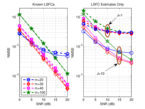
Figure 4: MSE of the proposed RR SSFC estimator using polynomial bases of various ranks; $\mathrm{AS}=7.2^{\circ}$. Theoretical MSE (LABEL:eqn:23) with known mean AoA is given (in solid lines) in the left plot. The right plot shows the SSFC estimation performance with LSFC estimated from $J=1$ or $10$ blocks.

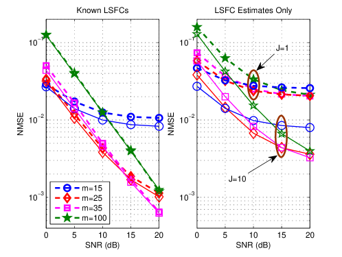
Figure 5: MSE of the proposed DCT-based SSFC estimator of various ranks; $\mathrm{AS}=7.2^{\circ}$. The right plot shows the SSFC estimation performance with LSFC estimated from $J=1$ or $10$ blocks, whereas theoretical MSE (LABEL:eqn:23) having known AoAs is given in the left plot (in solid lines).

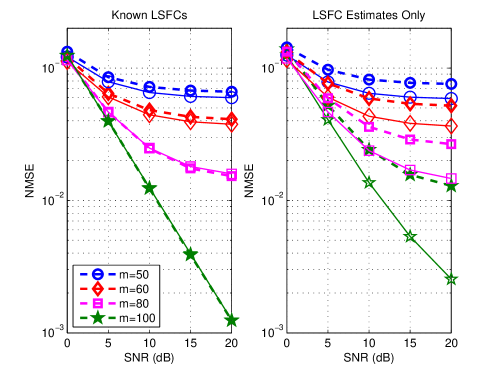
Figure 6: MSE of the proposed polynomial-based SSFC estimator with various ranks; $\mathrm{AS}=15^{\circ}$. Theoretical MSE (LABEL:eqn:23) with known mean AoA is given (in solid lines) in the left plot, while the MSE with LSFC estimated from $J=1$ and $10$ blocks in dashed and solid lines, respectively, in the right.

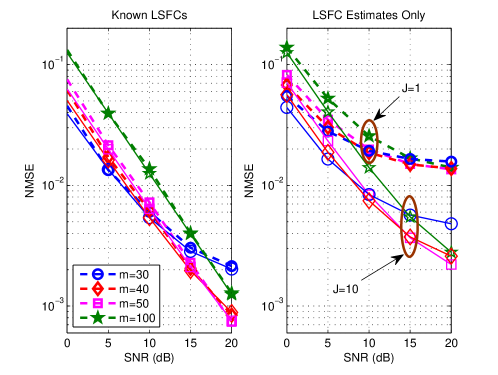
Figure 7: MSE of the proposed RR SSFC estimator using DCT bases of various ranks; $\mathrm{AS}=15^{\circ}$. Theoretical MSE (LABEL:eqn:23) with perfect mean AoA knowledge is given (in solid lines) in the left plot. The right plot shows the SSFC estimation performance with LSFC estimated from $J=1$ or $10$ blocks.

In addition, we study the SSFC estimation performance of $\hat{\mathbf{h}}^{(\textrm{II})}$ with respect to modeling order and basis matrix with estimated or perfectly-known $\boldsymbol{\beta}$ in Figs. 4–7. Since the spatial correlation increases with reducing AS, the spatial waveform of an MS over the array is anticipated to be smoother. As a result, when AS is comparatively small, due to over-modeling the channel vector the estimation performance not only cannot be improved, but also may be degraded. This is because the amount of available information does not grow with that of the parameters required to be obtained. As can be observed in Fig. 4, when LSFCs are perfectly known, the estimation accuracy with polynomial basis degrades as modeling order increases from $20$ to $100$ for $\mathrm{SNR}<5$ dB. Besides, the optimal modeling order increases with $\mathrm{SNR}$, e.g., optimal order at $\mathrm{SNR}=0$ and $5$ dB are respectively $20$ and $30$. Such result is observed due to the fact that MSE is noise-limited in the low SNR regime, while the importance of modeling error becomes more pronounced for high SNRs. Similar trend is also observed with DCT basis in Fig. 5.

On the other hand, when $\mathrm{AS}$ increases to $15^{\circ}$, the spatial correlation decreases and spatial waveforms roughen. As can be seen in Fig. 6, the SSFC estimator fails to capture these waveforms by using only some low-degree polynomials, and thus in this scenario, full modeling order ($M=100$) is required to achieve best performance for any SNR. However, DCT basis is still appropriate for parameter reduction due to the near-optimal energy-compacting capability od DCT as described Remark 11. In Fig. 7, we observe that when LSFCs are perfectly estimated, a modeling order of $30$ has the minimal MSE for $\mathrm{SNR}<9$ dB. Moreover, we can see from the right plots of Figs. 4–7 that the estimation of SSFCs requires accurate LSFC estimates. Such estimates can be easily obtained with multiple pilot blocks due to LSFCs’ slowly-varying characteristics.

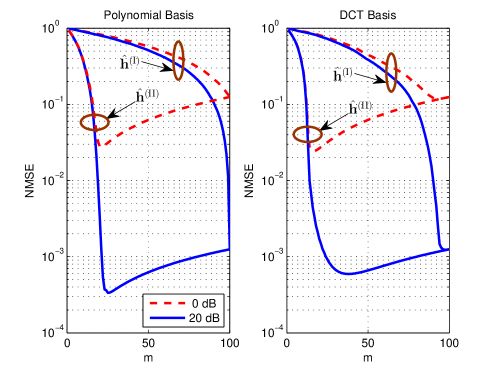
Figure 8: Theoretical MSE of $\hat{\mathbf{h}}^{(\textrm{I})}$ and $\hat{\mathbf{h}}^{(\textrm{II})}$ versus modeling order and $\mathrm{SNR}$; $\mathrm{AS}=7.2^{\circ}$.

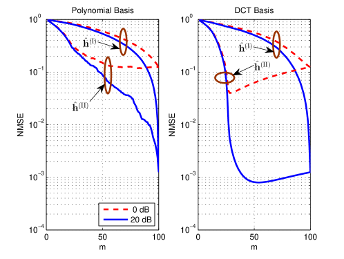
Figure 9: Theoretical MSE of $\hat{\mathbf{h}}^{(\textrm{I})}$ and $\hat{\mathbf{h}}^{(\textrm{II})}$ versus modeling order and $\mathrm{SNR}$; $\mathrm{AS}=15^{\circ}$.

Figs. 8 and 9 plot the theoretical MSE (LABEL:eqn:23) of the proposed two SSFC estimators with respect to the modeling order $m$ and compare the performance between $\hat{\mathbf{h}}^{(\textrm{I})}$ and $\hat{\mathbf{h}}^{(\textrm{II})}$ using a same basis matrix. While these plots are able to suggest some basis selecting guidance in different scenarios, they also substantiate the results shown in Figs. 4–7. First, we investigate the results of $\hat{\mathbf{h}}^{(\textrm{II})}$. When $\mathrm{AS}=7.2^{\circ}$, $\mathrm{SNR}=20$ dB, and, the polynomial basis is capable of rendering a better estimation performance with greater parameter number reduction than the DCT basis can provide, i.e., the optimal modeling order for the polynomial and DCT basis are respectively $25$ and $38$. However, when $\mathrm{SNR}$ reduces to $0$ dB, the DCT basis achieves the lowest MSE with $m=16$ as compared to $m=21$ of the polynomial basis. In spite of the effectiveness of the polynomial basis when $\mathrm{AS}=7.2^{\circ}$, it fails to represent channel with only a few low degree polynomials when $\mathrm{AS}=15^{\circ}$ and requires almost full order. On the other hand, the DCT basis is still applicable with optimal order $m=29$ and $54$ for $\mathrm{SNR}=0$ and $20$ dB, respectively.

As for $\hat{\mathbf{h}}^{(\textrm{I})}$, the fact that in the given scenarios its MSE performance is significantly worse than that of $\hat{\mathbf{h}}^{(\textrm{II})}$ for any $m$ and that the optimal order are all close to $M=100$ justifies our preference to $\hat{\mathbf{h}}^{(\textrm{II})}$. Recall that both $\hat{\mathbf{h}}^{(\textrm{I})}$ and $\hat{\mathbf{h}}^{(\textrm{II})}$ degenerate to the conventional LS estimator (42) if $m=100$, thus they all have the same performance regardless of the basis chosen. Although, applying the polynomial basis when $\mathrm{AS}=15^{\circ}$ causes performance inferior to that of the conventional LS estimator, $\hat{\mathbf{h}}^{(\textrm{I})}$ offers direct performance-complexity trade-off.

VI Conclusion

Taking advantage of the noise reduction effect and the large number of samples available in a massive MIMO system, we propose a novel LSFC estimator for both spatially-correlated and uncorrelated channels. This estimator is easily extendable to the case when multiple pilot blocks become available. The estimator is of low complexity, requires no prior knowledge of SSFCs and spatial correlation, and yields asymptotically diminishing MSE when the number of BS antennas becomes large enough.

Using the estimated LSFCs, we present an algorithm which performs joint SSFC and mean AoA estimation with rank-reduced channel model. The simultaneous mean AoA estimation not only offer useful information for downlink beamforming but also improves the SSFC estimator’s performance. A closed-form MSE expression for the proposed SSFC estimator is derived to investigate the rank reduction efficiency.

Moreover, we compare some candidate bases for RR representation and examine their effects on SSFC estimation. We show that the DCT basis is an excellent choice due to its low computing complexity and, more importantly to its energy compaction capability. Numerical results confirm the effectiveness of the proposed estimator and verify that the optimal modeling order is a function of AS and SNR.

Appendix Appendix A Proof of Theorem 1

Lemma 2 implies that if

$$\underset{{M\rightarrow\infty}}{\limsup}\underset{{1\leq i,j\leq K}}{\sup}\|\mathbf{\Phi}_{i}^{\frac{1}{2}}\mathbf{\Phi}_{j}^{\frac{1}{2}}\|_{2}<\infty,$$ (A.1)

we have

$$\frac{1}{M}\tilde{\mathbf{H}}^{H}\mathbf{A}\tilde{\mathbf{H}}$$

$$=\frac{1}{M}\left[\begin{array}[]{ccc}\tilde{\mathbf{h}}_{1}^{H}\mathbf{\Phi}_{1}^{\frac{1}{2}}\mathbf{\Phi}_{1}^{\frac{1}{2}}\tilde{\mathbf{h}}_{1}&\cdots&\tilde{\mathbf{h}}_{1}^{H}\mathbf{\Phi}_{1}^{\frac{1}{2}}\mathbf{\Phi}_{K}^{\frac{1}{2}}\tilde{\mathbf{h}}_{K}\\ \vdots&\ddots&\vdots\\ \tilde{\mathbf{h}}_{K}^{H}\mathbf{\Phi}_{K}^{\frac{1}{2}}\mathbf{\Phi}_{1}^{\frac{1}{2}}\tilde{\mathbf{h}}_{1}&\cdots&\tilde{\mathbf{h}}_{K}^{H}\mathbf{\Phi}_{K}^{\frac{1}{2}}\mathbf{\Phi}_{K}^{\frac{1}{2}}\tilde{\mathbf{h}}_{K}\end{array}\right]\stackrel{{\scriptstyle a.s.}}{{\longrightarrow}}\mathbf{I}_{K},$$ (A.5)

and if $\underset{{M\rightarrow\infty}}{\limsup}\underset{{1\leq i\leq K}}{\sup}\|\mathbf{\Phi}_{i}^{\frac{1}{2}}\|_{2}<\infty$,

$$\underset{{M\rightarrow\infty}}{\limsup}\underset{{1\leq i\leq K}}{\sup}\|\mathbf{\Phi}_{i}\|_{2} < \infty,$$ (A.7)

then

$$\frac{1}{M}\tilde{\mathbf{H}}^{H}\tilde{\mathbf{\Phi}}^{H}\mathbf{N}$$

$$=\frac{1}{M}\left[\begin{array}[]{ccc}\tilde{\mathbf{h}}_{1}^{H}\mathbf{\Phi}_{1}^{\frac{1}{2}}\mathbf{n}_{1}&\cdots&\tilde{\mathbf{h}}_{1}^{H}\mathbf{\Phi}_{1}^{\frac{1}{2}}\mathbf{n}_{K}\\ \vdots&\ddots&\vdots\\ \tilde{\mathbf{h}}_{K}^{H}\mathbf{\Phi}_{K}^{\frac{1}{2}}\mathbf{n}_{1}&\cdots&\tilde{\mathbf{h}}_{K}^{H}\mathbf{\Phi}_{K}^{\frac{1}{2}}\mathbf{n}_{K}\end{array}\right]\stackrel{{\scriptstyle a.s.}}{{\longrightarrow}}\mathbf{0}_{K\times T}.$$ (A.11)

Note that Assumption 1 is equivalent to (A.7) and implies (A.1) since if $\forall~{}i$, $\|\mathbf{\Phi}_{i}^{\frac{1}{2}}\|_{2}<\infty$, then

$$\|\mathbf{\Phi}_{i}^{\frac{1}{2}}\mathbf{\Phi}_{j}^{\frac{1}{2}}\|_{2}{\leq}\|\mathbf{\Phi}_{i}^{\frac{1}{2}}\|_{2}\|\mathbf{\Phi}_{j}^{\frac{1}{2}}\|_{2} < \infty,~{}\forall~{}1\leq i,j\leq K.$$

Appendix Appendix B Proof of Theorem 2

In the following, we derive the variance and bias terms of the MSE of $\hat{\mathbf{h}}^{(\textrm{II})}$. Those of the MSE of $\hat{\mathbf{h}}^{(\textrm{I})}$ can be similarly obtained. We start with the derivation of the variance term.

$$\mathrm{Var}\{\hat{\mathbf{h}}^{(\textrm{II})}\} = \mathbb{E}\left\{\left\|\hat{\mathbf{h}}^{(\textrm{II})}-\mathbb{E}\{\hat{\mathbf{h}}^{(\textrm{II})}\}\right\|^{2}\right\}~{}~{}~{}~{}$$

$$= \frac{1}{\gamma^{2}}\mathbf{p}^{H}\mathbb{E}\left\{\mathbf{N}^{H}\mathbf{W}(\hat{\phi})\mathbf{Q}_{m}^{(\textrm{II})}\left(\mathbf{Q}_{m}^{(\textrm{II})}\right)^{H}\mathbf{W}^{H}(\hat{\phi})\mathbf{N}\right\}\mathbf{p}$$

$$= \frac{1}{\gamma^{2}}\mathbf{p}^{H}\mathrm{tr}\left(\mathbf{W}(\hat{\phi})\mathbf{Q}_{m}^{(\textrm{II})}\left(\mathbf{Q}_{m}^{(\textrm{II})}\right)^{H}\mathbf{W}^{H}(\hat{\phi})\right)\mathbf{p}$$

$${=} \frac{1}{\gamma^{2}}\mathbf{p}^{H}(m\mathbf{I}_{K})\mathbf{p}=\frac{m}{\beta\|\mathbf{p}\|^{2}}$$

where we have invoked the relation

$$\mathbb{E}\left\{\mathbf{N}^{H}\mathbf{X}\mathbf{N}\right\} = \sum_{i=1}^{M}\sum_{j=1}^{M}x_{ij}\mathbb{E}\left\{\mathbf{n}_{i}\mathbf{n}_{j}^{H}\right\}$$ (B.2)

$$= \sum_{i=1}^{M}x_{ii}\mathbb{E}\left\{\mathbf{n}_{i}\mathbf{n}_{i}^{H}\right\}=\mathrm{tr}(\mathbf{X})\mathbf{I}_{K}~{}~{}~{}$$

with white noise $\mathbf{N}=\left[\mathbf{n}_{1},\cdots,\mathbf{n}_{M}\right]^{H}$ for any square matrix $\mathbf{X}=[x_{ij}]$. For the bias term, we have

$$b(\hat{\mathbf{h}}^{(\textrm{II})}) = \mathbb{E}\left\{\left\|\mathbb{E}\{\hat{\mathbf{h}}^{(\textrm{II})}\}-\mathbf{h}\right\|^{2}\right\}$$

$$= \mathbb{E}\left\{\mathbf{h}^{H}\left(\mathbf{W}(\hat{\phi})\mathbf{Q}_{m}^{(\textrm{II})}\left(\mathbf{Q}_{m}^{(\textrm{II})}\right)^{H}\mathbf{W}^{H}(\hat{\phi})-\mathbf{I}_{M}\right)^{2}\mathbf{h}\right\}$$

$$= \mathrm{tr}\left(\left(\mathbf{W}(\hat{\phi})\mathbf{Q}_{m}^{(\textrm{II})}\left(\mathbf{Q}_{m}^{(\textrm{II})}\right)^{H}\mathbf{W}^{H}(\hat{\phi})-\mathbf{I}_{M}\right)^{2}\mathbf{\Phi}\right)\vspace{-1em}$$

$$\hskip 16.99998pt\underbrace{\hskip 155.00023pt}_{\stackrel{{\scriptstyle def}}{{=}}\mathbf{A}_{1}}$$

Since

$$\mathbf{Q}_{m}^{(\textrm{II})}\left(\mathbf{Q}_{m}^{(\textrm{II})}\right)^{H} = \mathbf{Q}^{(\textrm{II})}\left[\begin{array}[]{c}\mathbf{I}_{m}\\ \mathbf{0}_{(M-m)\times m}\end{array}\right]\left[\mathbf{I}_{m}~{}\mathbf{0}_{(M-m)\times m}\right]\left(\mathbf{Q}^{(\textrm{II})}\right)^{H}$$ (B.5)

$$\stackrel{{\scriptstyle def}}{{=}} \mathbf{Q}^{(\textrm{II})}(\mathbf{I}_{M}-\mathbf{D}_{m})\left(\mathbf{Q}^{(\textrm{II})}\right)^{H}$$ (B.6)

where $\mathbf{D}_{m}=\mathrm{Diag}\left(\left[\mathbf{0}_{1\times m}~{}\mathbf{1}_{1\times(M-m)}\right]^{T}\right)$, we have $\mathbf{A}_{1}=\mathbf{W}(\hat{\phi})\mathbf{Q}^{(\textrm{II})}\mathbf{D}_{m}\left(\mathbf{Q}^{(\textrm{II})}\right)^{H}\mathbf{W}^{H}(\hat{\phi})$ and

$$b(\hat{\mathbf{h}}^{(\textrm{II})}) = \mathrm{tr}\left(\mathbf{W}(\hat{\phi})\mathbf{Q}^{(\textrm{II})}\mathbf{D}_{m}\left(\mathbf{Q}^{(\textrm{II})}\right)^{H}\mathbf{W}^{H}(\hat{\phi})\mathbf{\Phi}\right)$$ (B.7)

$$= \mathrm{tr}\left(\mathbf{D}_{m}\left(\mathbf{Q}^{(\textrm{II})}\right)^{H}\mathbf{W}^{H}(\hat{\phi})\mathbf{\Phi}\mathbf{W}(\hat{\phi})\mathbf{Q}^{(\textrm{II})}\right).~{}~{}~{}~{}$$

Appendix Appendix C On the Spatial Correlation

Following [7], we express the spatial correlation between two antenna elements in an array with arbitrary configuration as

$$[\mathbf{\Phi}]_{ij} = \mathbb{E}\{h_{i}h_{j}^{*}\}$$ (C.1)

$$= \int_{-\pi}^{\pi}p(\theta)\exp\left(j\mathbf{k}^{T}(\theta)(\mathbf{u}_{i}-\mathbf{u}_{j})\right)\mathrm{d}\theta$$

where $p(\theta)$ is the probability density function of AoA, $\mathbf{k}(\theta)=-\frac{2\pi}{\lambda}[\cos(\theta)~{}\sin(\theta)]^{T}$, and $\mathbf{u}_{i}=[u_{ix}~{}u_{iy}]^{T}$ represents the Cartesian coordinates of the $i$th antenna element. Without loss of generality, we assume antenna elements $i$ and $j$ lie on the y-axis and the impinging waveform spread over $[\phi-\Delta,\phi+\Delta]$. Thus, for small $\Delta$ and antenna spacing $d_{ij}\stackrel{{\scriptstyle def}}{{=}}{u}_{iy}-{u}_{jy}$, we have

$$[\mathbf{\Phi}]_{ij} = \int_{-\Delta}^{\Delta}p(\theta+\phi)e^{-j\frac{2\pi d_{ij}}{\lambda}\sin(\theta+\phi)}\mathrm{d}\theta$$

$$\approx e^{-j\frac{2\pi d_{ij}}{\lambda}\sin\phi}\int_{-\Delta}^{\Delta}p(\theta+\phi)e^{-j\frac{2\pi d_{ij}}{\lambda}\sin\theta\cos\phi}\mathrm{d}\theta.$$

The integral on the right hand side is real if $p(\theta)$ is symmetric about $\phi$ and for a system using ULA at the BS, $d_{ij}=(i-j)\xi$.

References

• [1] F. Rusek, D. Persson, B. K. Lau, E. G. Larsson, T. L. Marzetta, O. Edfors, and F. Tufvesson, โ€œScaling up MIMO: opportunities and challenges with very large arrays,โ€ IEEE Signal Proces. Mag., vol. 30, no. 1, pp. 40โ€“60, Jan. 2013.
• [2] S. Payami and F. Tufvesson, โ€œMeasured propagation characteristics for very-large MIMO at $2.6$ GHz,โ€ in Proc. ACSSC, Nov. 2012.
• [3] A. Liu and V. Lau, โ€œJoint power and antenna selection optimization in large distributed MIMO networks,โ€ Tech. Rep., 2012.
• [4] J. P. Kermoal, L. Schumacher, K. I. Pedersen, P. E. Mogensen, and F. Frederiksen, โ€œA stochastic MIMO radio channel model with experimental validation,โ€ IEEE J. Sel. Areas Commun., vol. 20, no. 6, pp. 1211โ€“1226, Aug. 2002.
• [5] J. Hoydis, S. ten Brink, and M. Debbah, โ€œMassive MIMO in the UL/DL of cellular networks: how many antennas do we need?,โ€ IEEE J. Sel. Areas Commun., vol. 31, no. 2, pp. 160โ€“171, Feb. 2013.
• [6] โ€œSpatial channel model for multiple input multiple output (MIMO) simulations,โ€ 3GPP TR 25.996 V11.0.0, Sep. 2012. [Online]. Available: http://www.3gpp.org/ftp/Specs/html-info/25996.htm
• [7] C.-X. Wang, X. Hong, H. Wu and W. Xu, โ€œSpatial-temporal correlation properties of the 3GPP spatial channel model and the Kronecker MIMO channel model,โ€ EURASIP J. Wireless Commun. and Netw., 2007.
• [8] H. Yin, D. Gesbert, M. Filippou, and Y. Liu, โ€œA coordinated approach to channel estimation in large-scale multiple-antenna systems,โ€ IEEE J. Sel. Areas Commun., vol. 31, no. 2, pp. 264โ€“273, Feb. 2013.
• [9] M. Biguesh and A. B. Gershman, โ€œTraining-based MIMO channel estimation: a study of estimator tradeoffs and optimal training signals,โ€ IEEE Trans. Signal Process., vol. 54, no.3, pp. 884โ€“893, Mar. 2006.
• [10] L. Rong, X. Su, J. Zeng, Y. Kuang, and J. Li, โ€œLarge scale MIMO transmission technology in the architecture of cloud base-station,โ€ in Proc. IEEE GLOBECOM Workshops, pp. 255โ€“260, Dec. 2012.
• [11] H. Q. Ngo, M. Matthaiou, and E. G. Larsson, โ€œPerformance analysis of large scale MU-MIMO with optimal linear receivers,โ€ Swedish Commun. Tech. Workshop (Swe-CTW), pp. 59โ€“64, Oct. 2012.
• [12] S. M. Kay, Fundamentals of Statistical Signal Processing: Estimation Theory, Prentice Hall, 1993.
• [13] J. Jose, A. Ashikhmin, T. Marzetta, and S. Vishwanath, โ€œPilot contamination problem in multi-cell TDD systems,โ€ in Proc. IEEE ISIT, pp. 2184โ€“2188, Jul. 2009.
• [14] โ€œEvolved universal terrestrial radio access (E-UTRA); further advancements for E-UTRA physical layer aspects,โ€ 3GPP TR 36.814 V9.0.0, Mar. 2010. [Online]. Available: http://www.3gpp.org/ftp/Specs/html-info/36814.htm
• [15] F. Fernandes, A. Ashikhmin and T. L. Marzetta, โ€œInter-Cell Interference in Noncooperative TDD Large Scale Antenna Systems,โ€ IEEE J. Sel. Areas Commun., vol. 31, no. 2, pp.192โ€“201, Feb. 2013.
• [16] R. Couillet and M. Debbah, Random Matrix Methods for Wireless Communications, New York, NY, USA: Cambridge University Press, 2011.
• [17] H. Huh, G. Caire, H. C. Papadopoulos, and S. A. Ramprashad, โ€œAchieving โ€œmassive MIMOโ€ spectral efficiency with a not-so-large number of antennas,โ€ IEEE Trans. Wireless Commun., vol. 9, no. 5, pp. 3226โ€“3238, Sep. 2012.
• [18] Z. D. Bai and J. W. Silverstein, Spectral Analysis of Large Dimensional Random Matrices, 2nd ed. Springer Series in Statistics, New York, NY, USA, 2009.
• [19] Y.-C. Chen and Y. T. Su, โ€œMIMO channel estimation in correlated Fading Environments,โ€ IEEE Trans. Commun., vol. 9, no. 3, pp. 1108โ€“1119, Mar. 2010.
• [20] D.-S. Shiu, G. J. Foschini, M. J. Gans, and J. M. Kahn, โ€œFading correlation and its effect on the capacity of multielementantenna systems,โ€ IEEE Trans. Commun., vol. 48, no. 3, pp. 502โ€“513, Mar. 2000.
• [21] A. M. Sayeed, โ€œDeconstructing multiantenna fading channels,โ€ IEEE Trans. Signal Process., vol. 50, no. 10, pp.2563-2579, Oct. 2002.
• [22] W. Weichselberger, M. Herdin, H. ร–zcelik, and E. Bonek, โ€œA stochastic MIMO channel model with joint correlation of both link ends,โ€ IEEE Trans. Wireless Commun., vol. 5, no. 1, pp. 90-100, Jan. 2006.
• [23] K. R. Rao and P. C. Yip, The Transform and Data Compression Handbook, CRC Press, Inc. Boca Raton, FL, USA, 2000.
• [24] P. R. Haddad, A. N. Akansu, Multiresolution Signal Decomposition, Second Edition: Transforms, Subbands, and Wavelets, Academic Press, Oct. 2000.
• [25] N. Ahmed, T. Natarajan, and K. R. Rao, โ€œDiscrete cosine transform,โ€ IEEE Trans. Comput., vol. C-23, no. 1, pp. 90โ€“93, 1974.
• [26] A. V. Oppenheim, R. W. Schafer, Discrete-Time Signal Processing: Third Edition, Pearson, 2010.