Excitations and quasi-one-dimensionality in field-induced nematic and spin density wave states

Abstract

We study the excitation spectrum and dynamical response functions for several quasi-one-dimensional spin systems in magnetic fields without dipolar spin order transverse to the field. This includes both nematic phases, which harbor “hidden” breaking of spin-rotation symmetry about the field and have been argued to occur in high fields in certain frustrated chain systems with competing ferromagnetic and antiferromagnetic interactions, and spin density wave states, in which spin-rotation symmetry is truly unbroken. Using bosonization, field theory, and exact results on the integrable sine-Gordon model, we establish the collective mode structure of these states, and show how they can be distinguished experimentally.

I Introduction

Much of the research in frustrated quantum magnets has focused on the elusive quest for magnetically disordered phases with highly entangled ground states: quantum spin liquids Balents (2010). Somewhat intermediate between these rare beasts and commonplace antiferromagnets are moderately exotic phases of antiferromagnets in strong magnetic fields which exhibit no dipolar magnetic order transverse to the field, contrary to typical spin-flop antiferromagnetic states. One such state, the Spin Nematic (SN), has received a particularly high degree of theoretical attention Andreev and Grishchuk (1984); Tsunetsugu and Arikawa (2006); Penc and Lauchli (2011). Argued to occur in some quasi-one-dimensional strongly frustrated insulators with competing ferromagnetic and antiferromagnetic interactions Chubukov (1991), the SN phase has a “hidden” order which breaks spin-rotation symmetry about the magnetic field despite the lack of transverse spontaneous local moments. A less celebrated but competitive state in such systems is the collinear Spin Density Wave (SDW) Starykh et al. (2010); Chen et al. (2013), which develops magnetic order but with spontaneous moments, whose magnitude is spatially modulated, entirely along the magnetic field direction. Both types of phases are strongly quantum, i.e. cannot occur in classical models with moments of fixed length at zero temperature. The absence of transverse moments in both phases may lead the two to be confused experimentally, and one of the reasons for the present study is to clearly define the characteristics that distinguish them in laboratory measurements.

A spin nematic is usually defined as a state without any spontaneous dipolar order, i.e. so that in a magnetic field along $z$, $\langle S_{i}^{+}\rangle=0$, but with quadrupolar order, $\langle S_{i}^{+}S_{j}^{+}\rangle\neq 0$, for nearby sites $i,j$. Such a nematic breaks the $U(1)$ spin rotation symmetry about the field axis, but in a more non-trivial way than a usual canted antiferromagnet. The spin nematics relevant to this paper are based on the frustrated Heisenberg chain with ferromagnetic nearest-neighbor coupling and antiferromagnetic second-neighbor coupling, in a strong magnetic field. For a region of parameters, the single magnon excitations with $S^{z}=\pm 1$ of the fully saturated high field state are bound into pairs with $S^{z}=\pm 2$. Roughly, these latter excitations “condense” upon lowering the field, leading to a spin nematic state Hikihara et al. (2008); Sudan et al. (2009); Zhitomirsky and Tsunetsugu (2010). Some caution should be exercised, however, since in one dimension true condensation is not possible, and spontaneous breaking of rotational symmetry about the field cannot occur. A sharp characterization of the one-dimensional (1d) spin nematic is, rather than nematic order, the presence of a gap to $S^{z}=\pm 1$ excitations. The 1d SN state may be thought of more properly as a bose liquid of $S^{z}=\pm 2$ particles, and hence has not only power-law nematic order but also power-law density fluctuations of those bosons Hikihara et al. (2008) (see Sec. II.2.2). The latter is just power-law SDW correlations. Inter-chain couplings can stabilize either long-range nematic or SDW order. One of our results is that, in fact SDW order is typically more stable, and true nematic long-range order occurs only in a narrow range of applied fields very close to the fully saturated magnetization.

More generally, SDW order also occurs in frustrated 1d systems from other mechanisms, unrelated to magnon pairing and 1d spin nematicity. Thus we will spend considerable time in this paper discussing the properties of the SDW. At the level of order parameter, an SDW state is described by the expectation value

$$\langle S_{i}^{z}\rangle=M+{\rm Re}\left[\Phi e^{i{\bf k}_{\rm sdw}\cdot{\bf r}_{i}}\right]+\cdots$$ (1)

where the ellipses represent higher order harmonics that may be present, or small effects from spin-orbit coupling etc. SDW states are are relatively common in itinerant systems with Fermi surface instabilities Grüner (1994), but much less so at low temperature in insulating spin systems, which tend to behave classically and hence possess magnetic moments of fixed length. From the point of view of symmetry, the SDW breaks no global symmetries (time reversal symmetry is broken and the $z$ axis is already selected by a magnetic field), but instead breaks translational symmetry. Consequently, its only low energy mode is expected to be the pseudo-Goldstone mode of these broken translations, known as a phason. The phason is a purely longitudinal mode, as it corresponds to the phase of $\Phi$ above and hence a modultion only of $S^{z}$. This is also unusual in the context of insulating magnets, as the low energy collective modes are usually spin waves, which are transverse excitations, associated with small rotations of the spins away from their ordered axes. In spin wave theory, indeed, longitudinal modes are typically expected to be highly damped, and hence either undefined or hard to observe Affleck and Wellman (1992); Schulz (1996). In SDW states, they can instead control the low energy spectral weight in a scattering experiment. The SDW state also has transverse excitations, as we discuss in Sec. III.2.2, but these exhibit a spectral gap which is generally non-zero. They can be distinguished from the phasons by their polarization and their location in momentum space.

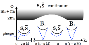
Figure 1: Schematic view of the excitation spectrum in the collinear SDW state (see Section III), i.e. the inelastic structure factor, in momentum (parallel to the chain direction defined by strong bonds) and energy space. Solid (black) lines show the results of chain mean field theory, i.e. excitations on single chains, and dashed (blue) lines give the two-dimensional results corrected for collective inter-chain effects (by the RPA approximation). The symbols $s$ (soliton), $\bar{s}$ (antisoliton) and $B_{1}$ (breather) on top of solid lines indicate their origin in the excitations of the single chain sine-Gordon model. The excitations shown here at momenta $k_{x}=\pi(1\pm 2M)$ and $k_{x}=0$ occur in the longitudinal ($S^{z}$) channel, while those at $k_{x}=\pi$ and $k_{x}=\pm 2\pi M$ occur in the transverse ($S^{\pm}$) one. Note that while all excitations are gapped at the sine-Gordon level (solid lines), the longitudinal excitations become gapless, reflecting the phason mode, once two-dimensional effects are included. The shaded gray area indicates a multi-particle continuum composed of solitons, antisolitons $(s,{\bar{s}})$ and breathers $B_{1}$. The figure is drawn for the situation $M<1/4$, for which $\pi(1-2M)$ is larger than $2\pi M$. For $M>1/4$, the corresponding features exchange places in the sketch.

In this paper, we focus primarily on the excitations of SDW and 2d spin nematic states. We show how to use the tools of one dimensional field theory, combined with the random phase approximation (RPA) and other methods to obtain both excitations and their contributions to different components of the dynamical and momentum dependent spin susceptibilities in a quantitative fashion. This analysis is greatly facilitated by the use of copious exact results on the excitations and correlation functions of the one dimensional sine-Gordon model Essler et al. (2003); Essler and Konik (2004); Gogolin et al. (2004). The results for the excitations of SDW states can also be easily extended to describe magnetization plateaux, which can be viewed as SDW states pinned by the commensurate lattice potential Starykh et al. (2010). Most of the results for SDW excitations carry over directly to such plateaux, with the main modification that the phason develops a small gap due to pinning.

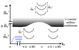
Figure 2: Schematic structure factor, analogous to Fig. 1, for the two dimensional spin nematic state (see Section IV). In contrast to the SDW case, only qualitative shifts of the excitations away from $k_{x}=0$ occur, so we draw only solid (black) lines there. Excitations at momenta $k_{x}=\pi(1\pm 2M)$ and $k_{x}=0$ are longitudinal, and those at $k_{x}=\pi$ are transverse (a gapped transverse mode at $2\pi M$ is also present, but not shown in the Figure). Note the absence of low energy transverse excitations. Indeed, as indicated by the break in vertical scale, excitations at $k_{x}=\pi$ exhibit a much larger gap in the spin nematic case, owing to the formation of this gap already at the decoupled chain level. The gapless Goldstone mode of the spin nematic, shown as a dashed (blue) line, contributes only in the vicinity of $k_{x}=0$. Vertical axes labels and energy separations refer to symbols from the treatment in Sec. IV.

In experiment, inelastic neutron scattering is a powerful way to study the SDW and 2d spin nematic states, and for convenience we summarize several distinguishing features identified from our analysis here. Both states have linearly dispersion gapless modes: phasons in the SDW case and the Goldstone modes (“quadrupolar waves”) in the nematic case Shindou et al. (2013); Bar’yakhtar et al. (2013); Smerald and Shannon (2013). In the structure factor, the phason appears with greatest weight at the SDW wavevector, which is in general incommensurate and away from the zone center and boundary. Here it gives a pole contribution whose weight diverges as $1/\omega$ as the energy of the pole approaches zero. The phason also contributes, although much more weakly, in the vicinity of the zone center, with a pole whose weight vanishes as the wave vector approaches zero. For the nematic, there is no divergent gapless contribution, and the gapless mode appears only at the zone center. The weights of the zone center contributions, though they both vanish on approaching $k=0$, differ in the angular dependence of the weight of the low energy pole. Another distinction is in the gapped portion of the spectrum. In the SDW case, the lowest gapped excitation, which carries a relatively large spectral weight, occurs usually at $k_{x}=\pi$, and occurs in the transverse ($S^{\pm}$) channel (a caveat here is that, in the SDW arising out of 1d spin nematic chains, this is not the case, and the transverse excitation at $k_{x}=\pi$ is pushed to high energy). In the nematic, the lowest energy gapped excitations occur instead at the incommensurate value $k_{x}=\pi(1\pm 2M)$, and excitations at $k_{x}=\pi$ appear only at much larger energies.

The rest of the paper is structured as follows. In Sec. II, we introduce bosonization and one-dimensional effective field theories in a general fashion which can be applied to both SDW and spin nematic states, in several different physical contexts. In Sec. III we derive the excitations and structure factor of the SDW phase, and in Sec. IV we do the same for the 2d nematic phase. We conclude in Sec. V with a Discussion of other ways to compare SDW and spin nematic phases, and of existing experiments. Several appendices contain technical details to support the results in the main text.

II One dimensional effective theory

In this section, we introduce the standard bosonization description which applies to many critical one dimensional systems, and establish notations to be used in the rest of the paper. A unified formalism of this type applies to several distinct physical situations, which we delineate below.

To justify the bosonization treatment, we will consider a quasi-one-dimensional geometry, composed of spin chains or ladders, coupled together by somewhat weaker exchange interactions between these one dimensional units. Each unit is characterized by some exchange scale $J$, presumed the largest in the problem, which sets a temperature scale $T_{\rm 1d}\sim J$, such that a low energy effective description of the one dimensional units applies for $T\lesssim T_{\rm 1d}$. Interactions amongst the one-dimensional units can them be described in terms of the low energy field theory, i.e. bosonization. These interactions, $J^{\prime}\ll T_{\rm 1d}$, induce ordering with a temperature $T_{\rm order}\sim J(J^{\prime}/J)^{b}\ll T_{\rm 1d}$, where the exponent $b>1$ is in general depedent upon more details of the interactions between and within the one-dimensional subsystems. Specific cases will be discussed below.

II.1 Bosonization for 1d Bose liquids

The low energy physics of a great variety of one dimensional spin systems can be described by bosonization in terms of free scalar bosonic field theory. We introduce one such field theory per one dimensional unit or chain, indexing these units by a discrete variable $y$. We presume $U(1)$ spin rotational symmetry about the $z$ axis, which allows but does not require a magnetic field along this axis.

Due to the $U(1)$ symmetry, we may view a spin-1/2 system as a Bose liquid, mapping for example the $S^{z}=-1/2$ state to the vacuum, the $S^{z}=+1/2$ state to a (hard core) boson, and thereby $S^{\pm}$ to boson creation/annihilation operators. The Bose liquid language has an advantage in that it allows for a unified view of ordinary antiferromagnetic spin chains and the more exotic one dimensional nematic (see below). Therefore we present first the bosonized form for the theory of a Bose liquid, and then give specific applications of this to different spin systems.

For a 1d Bose liquid, the fundamental operators are the density field $n_{y}(x)$ and creation/annihilation fields $\psi_{y}^{\dagger}(x),\psi_{y}^{\vphantom{\dagger}}(x)$, which are bosonized (yes, we are bosonizing bosons!) according to

$$n_{y}(x) = \overline{n}+\frac{1}{\beta}\partial_{x}\varphi_{y}-A_{1}\sin[\frac{2\pi}{\beta}\varphi_{y}(x)-k_{\rm sdw}x],$$

$$\psi_{y}(x) = A_{3}e^{-i\beta\theta_{y}(x)}+...$$ (2)

Here continuous $x$ runs along the chain, and we have introduced the slowly-varying “phase” fields $\varphi_{y}(x),\theta_{y}(x)$ which are continuous functions of $x$ and time $t$. The parameter $\beta$ depends upon details of the Bose liquid; it is also often convenient to introduce the “compactification radius” $R=\beta/(2\pi)$. $\beta$, or equivalently $R$, determines the long-distance behavior of the 1d correlation functions. The modulation wavevector $k_{\rm sdw}$ is that of an incipient Bose solid at the average Bose density $\overline{n}$, which is $k_{\rm sdw}=2\pi\overline{n}$. It is sometimes convenient to define the “charge density wave” order parameter for these bosons,

$$\Phi_{y}(x)=e^{-i\frac{2\pi}{\beta}\varphi_{y}},$$ (3)

so that

$$n_{y}(x)=\overline{n}+\frac{1}{\beta}\partial_{x}\varphi_{y}-\frac{iA_{1}}{2}\left(\Phi_{y}(x)e^{ik_{\rm sdw}x}-{\rm h.c.}\right).$$ (4)

For spin systems, $\Phi_{y}$ becomes the spin density wave order parameter. To keep the presentation symmetric, we also define the “superfluid” or XY order parameter $\Psi_{y}=e^{-i\beta\theta_{y}}$, so that

$$\psi_{y}(x)=A_{3}\Psi_{y}(x).$$ (5)

The conjugate fields $\varphi(x),\theta(x)$ obey the commutation relation

$$[\theta_{y}(x),\varphi_{y^{\prime}}(x^{\prime})]=-i\Theta(x-x^{\prime})\delta_{yy^{\prime}}.$$ (6)

where $\Theta(x)$ is the Heavyside step-function. Their dynamics is described by the free field Hamiltonian

$$H_{0}=\sum_{y}\int dx\frac{v}{2}\{(\partial_{x}\theta_{y})^{2}+(\partial_{x}\varphi_{y})^{2}\}.$$ (7)

This describes a single bosonic mode for each $y$: a central charge $c=1$ conformal field theory, also known as a Luther-Emery liquid or $c=1$ Luttinger liquid. The Hamiltonian contains a single parameter $v$, which gives the velocity of excitations which propagate relativistically, and which again depends upon microscopic details.

Such a Luttinger liquid is characterized by algebraic correlations, which are simply obtained from the above free field theory, the most prominent of which are

$$\langle n_{y}(x)n_{y}(0)\rangle_{c} = \frac{1}{2}A_{1}^{2}\cos[k_{\rm sdw}x]~{}|x|^{-2\Delta_{z}},$$ (8)

$$\langle\psi^{\vphantom{\dagger}}_{y}(x)\psi^{\dagger}_{y}(0)\rangle = A_{3}^{2}~{}|x|^{-2\Delta_{\perp}}.$$ (9)

Their power-law decay is controlled by the scaling dimensions $\Delta_{z}=\pi/\beta^{2}=1/(4\pi R^{2})$ and $\Delta_{\perp}=\beta^{2}/(4\pi)=\pi R^{2}$. Here we gave only the leading terms in (8) and (9), omitting corrections which decay faster with distance.

For the case of many spin chains, including the XXZ chain in a field along $z$, we can simply apply the above bosonization rules taking

$$S_{y}^{z}(x) = \frac{1}{2}-n_{y}(x),$$ (10)

$$S_{y}^{+}(x) = (-1)^{x}\psi_{y}(x).$$ (11)

In that case, $\overline{n}=1/2-M$, where $M$ is the uniform magnetization, and hence $k_{\rm sdw}=\pi-2\pi M$. For the isotropic Heisenberg chain, $2\pi R^{2}$ monotonically decreases from $1$ at zero magnetization ($M=0$) to $1/2$ at the full saturation $M=1/2$. This shows that in the presence of external magnetic field transverse spin fluctuations are more relevant (decay slower) than the longitudinal ones, $\Delta_{\perp}\leq\Delta_{z}$ for $0<M\leq 1/2$. At the same time the wave vector of longitudinal spin fluctuations shifts with magnetization continuously, as $k_{\rm sdw}=\pi(1-2M)$, toward the Brillouin zone center, while that of the transverse fluctuations, $k_{\perp}=\pi$, remains fixed at the Brillouin zone boundary.

As discussed above, two-dimensional order appears as a result of residual inter-chain interactions $J^{\prime}$ which are described by a perturbing Hamiltonian $H^{\prime}$. To understand under which conditions SDW can emerge from $H^{\prime}$, it is instructive to start by considering the simplest case of non-frustrated inter-chain coupling

$$H^{\prime}_{\rm non-fr}=J^{\prime}\sum_{x,y}{\bf S}_{y}(x)\cdot{\bf S}_{y+1}(x)\to$$

$$\to\sum_{y}\int dx~{}\gamma_{\rm sdw}\cos[2\pi(\varphi_{y}-\varphi_{y+1})/\beta]$$

$$+\gamma_{\rm xy}\cos[\beta(\theta_{y}-\theta_{y+1})].$$

Here we rewrote the first line in an appropriate low-energy form with the help of the representation (10), and we defined continuum inter-chain coupling constants $\gamma_{\rm sdw}=J^{\prime}A_{1}^{2}$ and $\gamma_{\rm xy}=J^{\prime}A_{3}^{2}$, which are of the same order. Since the fields on different chains are not correlated with each other at leading order (7), the scaling dimension $D$ of the SDW (cone) term in (II.1) is simply $D_{\rm sdw}=2\Delta_{z}(D_{\rm xy}=2\Delta_{\perp})$. Since in the case of isotropic Heisenberg chains $\Delta_{\perp}\leq\Delta_{z}$ for all $0<M\leq 1/2$, as argued above, the second term in the above equation becomes parametrically stronger than the first under the renormalization group (RG) flow. As a result, the interchain interaction (II.1) reduces to the xy term which implies two-dimensional order, via spontaneous $U(1)$ symmetry breaking, in the plane perpendicular to the external magnetic field. This is a familiar canted antiferromagnet, or spin-flop two sublattice ordered state. Note that $\langle S^{z}_{y}(x)\rangle$ is completely uniform in this phase.

The absence of an SDW phase noted here clearly follows from the condition $D_{\rm sdw}>D_{\rm xy}$. We observe that this may break down in three ways. First, for spin chains other than the simple Heisenberg one, the inequality $\Delta_{\perp}<\Delta_{z}$ may be violated in favor of the opposite situation. Second, for yet more exotic spin chains (or ladders), the relation between spin operators and those of the effective Bose gas may differ from that in Eqs. (10). Finally, third, the interactions between chains may differ from those in Eq. (II.1). We will encounter all these situations below.

II.2 Physical realizations

We now consider three different microscopic lattice models that lead to dominant SDW interactions. These models represent physically different ways of achieving the inequality $D_{\rm sdw}\leq D_{\rm xy}$. In general, the models we consider have, in their bosonized continuum limits, a Hamiltonian of the form $H=H_{0}+H^{\prime}$, with $H_{0}$ describing decoupled chains as in Eq. (7), and the inter-chain coupling of the form

$$H^{\prime} = \sum_{y}\int\!dx\,\Big{\{}\tfrac{1}{2}\gamma_{\rm sdw}\left(\Phi_{y}^{\dagger}\Phi_{y+1}^{\vphantom{\dagger}}+\Phi_{y+1}^{\dagger}\Phi_{y}^{\vphantom{\dagger}}\right)$$ (13)

$$+\tfrac{1}{2}\gamma_{\rm xy}\left(\Psi_{y}^{\dagger}\Psi_{y+1}^{\vphantom{\dagger}}+\Psi_{y+1}^{\dagger}\Psi_{y}^{\vphantom{\dagger}}\right)$$

$$+\tfrac{1}{2}\gamma^{\prime}_{\rm xy}\left(\Psi_{y}^{\dagger}i\partial_{x}\Psi_{y+1}^{\vphantom{\dagger}}-\Psi_{y+1}^{\dagger}i\partial_{x}\Psi_{y}^{\vphantom{\dagger}}\right).$$

The different models are distinguished by the values of the couplings $\gamma_{\rm sdw},\gamma_{\rm xy},\gamma^{\prime}_{\rm xy}$ and by the value of the chain interaction parameter $\beta$.

model	$\gamma_{\rm sdw}$	$\gamma_{\rm xy}$	$\gamma^{\prime}_{\rm xy}$
Ising chains	$\tfrac{1}{2}J^{\prime}\delta A_{1}^{2}$	$J^{\prime}A_{3}^{2}$	0
nematic chains	$\tfrac{1}{2}J^{\prime}A_{1}^{2}$	$\sim(J^{\prime})^{2}/J$	$0$
triangular lattice	$J^{\prime}A_{1}^{2}\sin(\pi M)$	$0$	$J^{\prime}A_{3}^{2}/2$

Table 1: Parameters describing three different physical realizations of the quasi-one-dimensional SDW state.

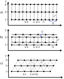
Figure 3: Lattice geometries considered in the paper. (a) Rectangular geometry, relevant for Ising-like coupled chains, discussed in Sec. II.2.1, and also for nematic chains, considered in Sec. II.2.2. In the latter case $J_{1}<0$ and $J_{2}>0$. (b) Equivalent representation of coupled nematic chains as a system of coupled zig-zag ladders. (c) Spatially anisotropic triangular lattice, discussed in Section II.2.3.

II.2.1 Ising anisotropy

The most straightforward route to $D_{\rm sdw}\leq D_{\rm xy}$ is provided by arranging $\Delta_{\perp}>\Delta_{z}$. This occurs by keeping the same unfrustrated rectangular arrangement of spin-1/2 chains discussed above, but replacing the Heisenberg chains with XXZ ones with Ising anisotropy,

$$H_{\rm Ising} = J\sum_{x,y}(S^{x}_{x,y}S^{x}_{x+1,y}+S^{y}_{x,y}S^{y}_{x+1,y}+\delta S^{z}_{x,y}S^{z}_{x+1,y}),$$

$$+ J^{\prime}\sum_{x,y}(S^{x}_{x,y}S^{x}_{x,y+1}+S^{y}_{x,y}S^{y}_{x,y+1}+\delta S^{z}_{x,y}S^{z}_{x,y+1}),$$

where $\delta>1$ parameterizes Ising anisotropy, and for simplicity we have taken the same anisotropy in the inter-chain coupling $J^{\prime}$, though this is not very important. In zero magnetic field, even in the absence of inter-chain coupling, such a chain orders spontaneously (at zero temperature, $T=0$) into one of the two Néel states, with spins ordered along the easy Ising ($z$) axis. The the non-frustrated interchain exchange $J^{\prime}$ then immediately selects the staggered arrangement of Néel order of adjacent chains, further stabilizing the antiferromagnet for low but non-zero temperature.

However, a sufficiently strong magnetic field, applied along the $z$ axis, breaks the gap, driving the XXZ chains into gapless Luttinger liquid state again Okunishi and Suzuki (2007). For small $J^{\prime}$, the problem can then be treated by bosonization and has the general form found above in Eq. (13), with $\gamma_{\rm sdw}=J^{\prime}\delta A_{1}^{2}/2$, $\gamma_{\rm xy}=J^{\prime}A_{3}^{2}$, and $\gamma^{\prime}_{\rm xy}=0$. More importantly, the Ising anisotropy increases $\beta$ relative to the Heisenberg chain. Indeed, it turns out that the critical indices of this state (parametrized in Okunishi and Suzuki (2007) by $\eta$ instead of our $R$) do have the desired property that $\Delta_{z}<\Delta_{\perp}$ for $M$ in the finite range $0<M\leq M_{c}(\delta)$. The critical magnetization $M_{c}(\delta)$, separating $\Delta_{z}<\Delta_{\perp}$ and $\Delta_{z}>\Delta_{\perp}$ regimes, increases with increasing anisotropy $\delta>1$.

It is clear that interchain interaction then stabilizes the two-dimensional SDW state in (approximately) the same magnetization interval $0<M\leq M_{c}(\delta)$ because here $\Delta_{z}<\Delta_{\perp}$ immediately implies $D_{\rm sdw}<D_{\rm cone}$. The exact value of the critical magnetization separating the two-dimensional SDW and cone states (with non-zero $J^{\prime}$) depends on many details and is not rigorously known. A reasonable estimate can be made by the chain mean field theory (CMFT), using the precise forms of the longitudinal and transverse spin susceptibilities as well as small (of the order $J^{\prime}/J\ll 1$) corrections to magnetization $M$ caused by the interchain exchange $J^{\prime}$. We disregard all these complications in order not to overload the discussion.

It appears that spin-1/2 antiferromagnet BaCo₂V₂O₈ realizes exactly this situation Kimura et al. (2008a). Static SDW order has been observed in several neutron and sound-attenuation studies (refs).

II.2.2 Spin-nematic chains

A second route to the collinear SDW is to suppress the leading xy instability altogether, by driving the individual spin chain into a completely different phase. This occurs in the model derived from LiVCuO₄, in which the one-dimensional chains are not XXZ like but instead incorporate ferromagnetic nearest-neighbor exchange $J_{1}<0$ and antiferromagnetic next-nearest exchange $J_{2}>0$ Enderle et al. (2005); Nishimoto et al. (2012). Such $J_{1}-J_{2}$ chains (which can also be “folded” into zig-zag ladders) have distinct behavior which is not captured by Eqs. (10).

Extensive research into this interesting chain geometry, dating back to 1991 Chubukov (1991), has found that the spectrum of the fully magnetized chain contains, in addition to usual single magnon states, tightly bound magnon pairs (in fact, three- and four-magnon complexes exists in some parameter range as well Hikihara et al. (2008); Sudan et al. (2009)). Importanly, these two-magnon pairs lie below the two-magnon continuum. As the magnetic field is reduced to the critical $h_{\rm sat}$ one, the gap for the two-magnon states vanishes while the single magnon gap remains non-zero. For $h<h_{\rm sat}$, therefore, one obtains not a Bose liquid of single magnons (which is the physical content of Eqs. (10)), but rather a Bose liquid of magnon pairsHikihara et al. (2008); Sato et al. (2013). In such a liquid, Eqs. (10) is replaced by

$$S_{y}^{z}(x) \sim \frac{1}{2}-2n_{y}(x),$$

$$S_{y}^{+}(x)S_{y}^{+}(x+1) \sim \psi_{y}(x).$$ (15)

where now $\psi_{y}(x)$ annihilates a magnon pair, and $n_{y}(x)$ counts the magnon pairs. The appearance of the operator quadratic in $S^{+}_{y}$ above indicates the existence of critical “spin nematic” correlations. Since a gap for single magnons (single spin flips) remains, the low energy projection of the single spin-flip operator vanishes

$$S_{y}^{\pm}(x)\sim``0".$$ (16)

For a single $J_{1}-J_{2}$ chain, this is still a Luttinger liquid state, but simple XY correlations decay exponentially instead of as a power law. The density correlations in this Bose liquid remain critical, and hence from Eq. (II.2.2) so do those of $S^{z}_{y}(x)$.

With this understanding, we see that even simple unfrustrated $J^{\prime}$ exchange interactions coupling the $J_{1}-J_{2}$ chains are “projected” onto dominantly Ising $S^{z}_{y}$ interactions, which strongly favor an SDW ground state. Specifically, we have again the form in Eq. (13), but with $\gamma_{\rm sdw}\sim J^{\prime}A_{1}^{2}\gg\gamma_{\rm xy}\sim(J^{\prime})^{2}/J$ and $\gamma^{\prime}_{\rm xy}=0$. The strong suppression of all single spin-flip operators suggests that, unlike in the previous case, the SDW state extends up to very close to the saturation value $M\sim 1/2$.

Unusual functional form of $\gamma_{\rm xy}\sim(J^{\prime})^{2}/J$ is due to the fact that it describes coupling of the nematic fields $\psi_{y}(x)$ of different chains. Such a coupling, involving four spin operators, see (II.2.2), is simply absent in the lattice model. It is, however, generated by quantum fluctuations in second order in the inter-chain exchange, which explains its peculiar form (the proportionality constant is non-trivial Sato et al. (2013) and not determined here). We will see that this can stabilize a true 2d SN near the saturation field – see Sec. IV.2. But away from a narrow region near saturation, the SDW state indeed dominates as naïvely expected.

II.2.3 Spatially anisotropic triangular lattice antiferromagnet

In the above two examples, we modified the interactions on the individual chains from the Heisenberg type. A third way to stabilize the SDW phase is to retain the simple nearest-neighbor Heisenberg form for the chain Hamiltonian, but modify explicitly the interactions between chains in a manner that frustrates the competing XY order. This occurs naturally for the situation of a spatially anisotropic triangular lattice Starykh and Balents (2007); Starykh et al. (2010). In this case, each spin is coupled symmetrically to two neighbors on adjacent chains, which frustrates the inter-chain interactions. Specifically, the interchain coupling reads

$$H^{\prime}_{\rm frust} =$$

$$J^{\prime}\sum_{x,y}{\bf S}_{y}(x)\cdot({\bf S}_{y+1}(x-1/2)+{\bf S}_{y+1}(x+1/2)).$$

Note that this Hamiltonian is written in a cartesian basis in which spins on, say, odd chains are located at the integer positions $x$ while those on the even chains are at the half-integer locations $x+1/2$. Bosonization of (II.2.3) gives again the form of Eq. (13), but with $\gamma_{\rm xy}=0$ due to frustration. The other two interactions are $\gamma_{\rm sdw}=J^{\prime}A_{1}^{2}\sin(\pi M)$ and $\gamma^{\prime}_{\rm xy}=J^{\prime}A_{3}^{2}/2$.

The SDW term retains its form but its coupling constant reflects frustration as well, $\gamma_{\rm sdw}\sim\sin[\pi M]\to 0$ for $M\to 0$. The SDW coupling resists the appearance of the derivative which occurs for the XY term, as a result of the shift of the longitudinal wave vector $k_{z}=\pi(1-2M)$ from its commensurate value $\pi$ for finite $M\neq 0$. It is this shift that makes SDW interaction more relevant than the XY one. While the SDW scaling dimension remains $D_{\rm sdw}=2\Delta_{z}$, that of the XY interaction increases to $D_{\rm xy}=1+2\Delta_{\perp}$. The addition of $1$ reflects the derivative in the $\gamma^{\prime}_{\rm xy}$ term of Eq. (13).

Since $D_{\rm sdw}=2\Delta_{z}<D_{\rm xy}=1+2\Delta_{\perp}$ in a rather wide range of magnetization, approximately for $0<M\leq 0.3$, interchain frustration stabilizes collinear SDW order Starykh et al. (2010).

III Excitations of collinear SDW state

In this section, we discuss the excitation spectrum of the collinear SDW state, and its manifestation in the magnetic structure factor (or wavevector dependent spin susceptibility). The magnetic excitations are collective modes, strongly influenced by symmetry. In an applied magnetic field, the only symmetries of the Hamiltonian are $U(1)$ rotation symmetry about the field, and the space group symmetries of the lattice. Notably, the collinear SDW state preserves the former $U(1)$ symmetry, and in the absence of broken continuous symmetry, lacks a Goldstone mode. Thus there are no acoustic transverse spin waves. Instead, we expect gapped transverse excitations. Given the highly quantum nature of the SDW phase in the quasi-1d, $S=1/2$ situation discussed here, there is in fact no a priori reason these excitations may be treated semiclassically in the traditional spin wave fashion. Instead, in the following, we will obtain the gapped excitations from a purely quantum treatment based on knowledge of the integrable 1d sine-Gordon model.

The collinear SDW does, however, break translation symmetry, and in particular exhibits incommensurate order (see Eq. (1)). Although translational symmetry is discrete, in cases of incommensurate order it is known to behave in some respects like a continuous symmetry and consequently the collinear SDW state supports a phason mode, which is the “pseudo-Goldstone” mode of broken translation symmetry. Physically this mode – which is acoustic – appears because of the vanishing energy cost for uniformly “sliding” the incommensurate density wave. In the bosonization framework, the elevation of the discrete lattice translation symmetry to an effectively continuous one appears in an emergent continuous symmetry of Eq. (II.1): invariance under $\varphi_{y}(x)\to\varphi_{y}(x)+\varphi^{(0)}$. While it is well-known in SDW-ordered metals, the phason excitation is perhaps less familiar in magnetically ordered insulators. We now turn to the detailed exposition of the excitation spectrum, including both phason and gapped modes. For simplicity, we focus here on zero-temperature ($T=0$) properties and apply CMFT to the problem. An alternative derivation of the phason dispersion, based on the Ginzburg-Landau (GL) action, is sketched in Appendix B.

III.1 Single chain excitations

In this subsection, we present the chain mean field theory which approximates the problem of the 2d system by a self-consistent set of independent chains, specifically 1+1d sine-Gordon models. We describe the gapped excitations occuring within individual such chains. The effects of two-dimensionality on the spectrum, and especially the emergence of the low energy phason mode, is discussed in the following subsection.

III.1.1 Chain mean field theory

Focusing on the SDW state, we drop the $\gamma_{\rm xy}$ and $\gamma^{\prime}_{\rm xy}$ terms in Eq. (13), and make the mean field replacement $H^{\prime}\rightarrow H^{\prime}_{\rm MF}$ (neglecting a constant), with

$$H^{\prime}_{\rm MF} \rightarrow =\sum_{y}\int\!dx\,\tfrac{1}{2}\gamma_{\rm sdw}\big{(}\langle\Phi_{y}^{\dagger}\rangle\Phi_{y+1}^{\vphantom{\dagger}}+\Phi_{y}^{\dagger}\langle\Phi_{y+1}^{\vphantom{\dagger}}\rangle$$ (18)

$$+\langle\Phi_{y+1}^{\dagger}\rangle\Phi_{y}^{\vphantom{\dagger}}+\Phi_{y+1}^{\dagger}\langle\Phi_{y}^{\vphantom{\dagger}}\rangle\big{)}-{\rm const.}.$$

With the ansatz

$$\langle\Phi_{y}\rangle=\overline{\Phi}(-1)^{y},$$ (19)

we then obtain

$$H^{\prime}_{\rm MF} = -\gamma_{\rm sdw}\overline{\Phi}\sum_{y}\int\!dx\,(-1)^{y}\left(\Phi_{y}^{\vphantom{\dagger}}+\Phi_{y}^{\dagger}\right),$$ (20)

where we took $\overline{\Phi}$ real.

The chain mean field theory (CMFT) has now reduced the system to a problem of decoupled chains. It can be brought into a simple standard form by expressing it in terms of the bosonized fields, and making the shift $\varphi_{y}\to\varphi_{y}+\beta y/2$, which gives finally $H_{0}+H^{\prime}_{\rm MF}=\sum_{y}H_{\rm sG}[\theta_{y},\varphi_{y}]$, where

$$H_{\rm sG}=\int dx~{}\frac{v}{2}[(\partial_{x}\varphi)^{2}+(\partial_{x}\theta)^{2}]-2\mu\cos[\frac{2\pi}{\beta}\varphi].$$ (21)

Here $\mu=\gamma_{\rm sdw}\overline{\Phi}$ and the self-consistency requirement in Eq. (19) becomes

$$\overline{\Phi}=\left\langle e^{i\frac{2\pi}{\beta}\varphi}\right\rangle_{\rm sG}=\left\langle\cos\frac{2\pi}{\beta}\varphi\right\rangle_{\rm sG}.$$ (22)

Our notation here closely follows Refs.[Essler and Konik, 2004; Gogolin et al., 2004], which describe many technical details important for the subsequent analysis.

III.1.2 Mass spectrum of the sine-Gordon model

The excitations of the sine-Gordon model in the massive phase ($\beta^{2}>\pi/2$) come in two varieties: solitons and antisolitons, which are domain walls connecting degenerate vacua (minima of the cosine), and breathers, which are bound states of solitons and antisolitons. The number of breathers is determined by the dimensionless parameter $\xi=1/(8\pi R^{2}-1)$, such that $n\leq[1/\xi]$ ($[x]$ denotes closest to $x$ integer such that $[x]\leq x$). The minimum energy of each breather – the mass in the relativistic sense – is given by the formula

$$m_{n}=2m_{s}\sin[\frac{\pi}{2}\xi n]~{}\text{for}~{}n=1,2,...[\frac{1}{\xi}],$$ (23)

expressed here in terms of the fundamental soliton mass $m_{s}$.

In the case of the spatially anisotropic triangular lattice, $\xi$ ranges from $1/3$ at $M=0$ to $1$ at the saturation, $M=1/2$. The breather masses are plotted in Fig. 4 versus $M$. For $0<M<0.125$, there are two breather modes. When the magnetization is increased to this value, the upper breather reaches the energy of the two-soliton continuum and merges with it. Hence, when $0.125<M<0.5$, there is only a single breather.

The soliton mass $m_{s}$ is determined by the coupling constant $\mu$ via the exact relation, Zamolodchikov (1995)

$$\mu = \frac{v\Gamma(\frac{1}{8\pi R^{2}})}{\pi\Gamma(1-\frac{1}{8\pi R^{2}})}\Big{(}\frac{m_{s}}{v}\frac{\sqrt{\pi}\Gamma(\frac{1+\xi}{2})}{2\Gamma(\frac{\xi}{2})}\Big{)}^{2-1/(4\pi R^{2})}$$ (24)

$$\sim v(m_{s}/v)^{2-1/(4\pi R^{2})}.$$

The scaling shown in the second line can be understood by simple renormalization group arguments. The relevant cosine operator in (21) grows under the RG according to $\mu(\ell)=\mu(0)\exp[(2-1/(4\pi R^{2}))\ell]$, where $\mu(0)\equiv\mu$ is the initial value of the coupling constant and $\ell$ is the logarithmic RG variable, so that the running energy scale is $\epsilon\sim ve^{-\ell}$. The coefficient $\mu(\ell)$ reaches strong coupling at $\ell_{0}$ such that $\mu(\ell_{0})=v$. Solving this for $\ell_{0}$, one obtains the energy $m_{s}\sim ve^{-\ell_{0}}$, which indeed matches the last line of (24). The value of the the exact solution in the first line of (24) is that it also provides with exact numerical prefactor.

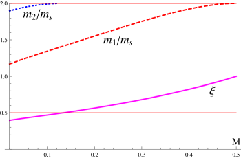
Figure 4: Plot of $\xi$ (solid (magenta) line) and breather masses $m_{1}/m_{s}$ (dashed (red) line) and $m_{2}/m_{s}$ (dotted (blue) line) as a function of magnetization $M$. Horizontal $y=0.5$ line is used to highlight “high magnetization” region with $[1/\xi]=1$: note that the second breather is absent there.

III.1.3 Self-consistency

To determine the overall scale of the excitation spectrum, we require the soliton mass $m_{s}$ or $\mu$. This is obtained from the self-consistency condition $\mu=\gamma_{\rm sdw}\overline{\Phi}$. The expectation value defining $\overline{\Phi}$ is readily obtained from the relation

$$\overline{\Phi} = =-\frac{1}{2}\frac{\partial F(\mu)}{\partial\mu},$$ (25)

where $F(\mu)$ is the ground state energy density of $H_{sG}$. Eq. (25) follows from first order perturbation theory in changes of $\mu$.

At the scaling level, as it is an energy density, we expect $F\sim vm_{s}^{2}$, and using Eq. (24) one obtains

$$m_{s}\sim v(\gamma_{\rm sdw}/v)^{2\pi R^{2}/(4\pi R^{2}-1)}.$$ (26)

This power can be understood from RG arguments, which indicate it is correct beyond CMFT. Under the RG, the SDW coupling grows according to $\gamma_{\rm sdw}(\ell)\sim\gamma_{\rm sdw}e^{(2-D_{\rm sdw})\ell}$, with $D_{\rm sdw}=2\Delta_{z}=1/(2\pi R^{2})$, which defines a scale $\ell_{0}$ by the condition that $\gamma_{\rm sdw}(\ell)$ reaches strong coupling, i.e. becomes of order $v$. Then using $m_{s}\sim ve^{-\ell_{0}}$, we obtain Eq. (26).

To go beyond scaling and obtain the prefactor and hence an absolute number for $m_{s}$, we turn to the exact solution of the sine-Gordon model. The standard result in the literature is $F_{\rm standard}=-m_{s}^{2}\tan[\pi\xi/2]/4$. It is, however, insufficient in the present case due to the obvious (and unphysical) divergence of $F_{\rm standard}$ in the $\xi\to 1$ ($4\pi R^{2}\to 1$) limit, i.e. in the limit of $M\to 1/2$.

This divergence is analyzed and cured, with the help of nominally less relevant terms, in the Appendix A. We present the result here. To obtain the soliton mass, one first solves for $\mu$ from the equation

$$(\frac{\mu}{v})^{1-\xi}=\frac{1+\xi}{8}\tan[\frac{\pi\xi}{2}]A_{1}^{2}A_{2}^{1+\xi}(\frac{\gamma_{\rm sdw}}{v})\times$$ (27)

$$\times\Big{(}1-\frac{1}{8}\tan[\frac{\pi}{1+\xi}]A_{1}^{\frac{4}{(1+\xi)}}A_{2}^{2}~{}Q^{\frac{(1-\xi)}{(1+\xi)}}(\frac{\gamma_{\rm sdw}}{v})\Big{)}^{-1}.$$

The soliton mass is then obtained as

$$m_{s}=vA_{1}\Big{(}\frac{\mu}{v}A_{2}\Big{)}^{(1+\xi)/2}.$$ (28)

This procedure allows us to explicitly determine the soliton mass $m_{s}$ as a function of $M$ for a given coupling constant $\gamma_{\rm sdw}$ of the original spin problem. For illustrative purposes, we plot the result for the case of the spatially anisotropic triangular lattice, for which $\gamma_{\rm sdw}=J^{\prime}A_{1}^{2}\sin[\pi M]$, with $J^{\prime}/J=0.5$ (chosen arbitrarily) in Figure 5.

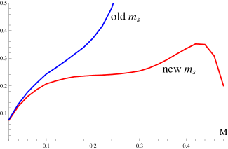
Figure 5: Plot of soliton mass $m_{s}/v$ as function of magnetization $M$ for $J^{\prime}=0.5J$. “Old $m_{s}$” (blue curve) is obtained using $F_{\rm standard}$, without correcting for $\xi\to 1$ divergence. “New $m_{s}$” (red curve) is corrected result (28), which is obtained using $F_{\rm new}$ from the Appendix A. For the spatially anisotropic triangular lattice the SDW phase, for which $m_{s}$ is calculated here, is the ground state of the 2d problem in the interval $0<M\lesssim 0.3$. At higher $M$ the SDW is replaced by the cone phase. Note that, in the limit $J^{\prime}/J\rightarrow 0$, at fixed $M$, the two curves converge to one another (in fact the ratio of $m_{s}$ calculated in both fashions converges to one).

III.2 Spin susceptibilities

The aim of this subsection is to show how the excitations described in the prior section, which are excitations already on a single chain, and the collective modes, which appear only when the full 2d dynamics are considered, appear in the physical dynamical susceptibilities, i.e. the components of the dynamical structure factor measured in inelastic neutron scattering. Formally these are defined as the linear response quantities,

$$X_{\mu\nu}({\bf k},\omega)=\left.\frac{\delta S^{\mu}({\bf k},\omega)}{\delta h^{\nu}({\bf k},\omega)}\right|_{{\bf h}({\bf k},\omega)=0},$$ (29)

where ${\bf h}$ is an oscillating infinitesimal applied Zeeman field at wavevector ${\bf k}$ and frequency $\omega$. By the usual linear response theory, this is minus the retarded correlation function of spin operators

$$X_{\mu\nu}({\bf k},\omega)\sim i\int_{0}^{\infty}\!dt\,e^{(i\omega-\epsilon)t}\left\langle\left[S^{\mu}({\bf k},t),S^{\nu}(-{\bf k},0)\right]\right\rangle,$$ (30)

where $\epsilon=0^{+}$.

We distinguish two types of susceptibilities. The longitudinal susceptibility describes the dynamical correlations of spin components $S^{z}$ along the applied field and the SDW polarization. Using the bosonization rule of Eqs. (4) and (10), we see that this is related to correlations of the SDW order parameter $\Phi$. Hence we define the bosonized equivalent, $\chi^{\rm zz}$, of the longitudinal susceptibility

$$X_{zz}({\bf k}=(k_{\rm sdw}+q,\pi+q_{y}),\omega)\sim\chi^{\rm zz}(q,q_{y},\omega),$$ (31)

and hence

$$\chi^{\rm zz}(q,q_{y},\omega) = i\int_{0}^{\infty}\!\!\!\!\!dt\!\!\int\!\!dx\sum_{y}\,e^{iqx+iq_{y}y+(i\omega-\epsilon)t}$$ (32)

$$\times\left\langle\left[\Phi_{y}(x,t),\Phi_{0}^{\dagger}(0,0)\right]\right\rangle.$$

Note that in $\chi^{zz}(q,q_{y},\omega)$, $q$ gives the shift of the momentum along the chain from the SDW one, i.e. $k_{x}=k_{\rm sdw}+q$, while $q_{y}$ is measured from $\pi$ due to the shift of $\varphi$ field by $\beta y/2$ made in deriving (21). Moreover, the continuum formula in Eq. (32) describes only the contributions to the susceptibility at low energy near $k_{x}=k_{\rm sdw},k_{y}=\pi$. Other contributions may apply elsewhere. For example, contribution from the vicinity of $k_{x}=-k_{\rm sdw},k_{y}=\pi$ is described by the hermitian conjugate of the expression in Eq. (32), while in that near $k_{x}=0$, the operator $\partial_{x}\varphi_{y}$ in Eq. (II.1) or Eq.(4) contributes. We neglect it here because, since this operator has larger scaling dimension than $\Phi_{y}$, it gives a subdominant contribution in the sense of smaller integrated weight in $X_{zz}$ (i.e. the weight near $k_{x}=0$ is smaller than that near $k_{x}=\pm k_{\rm sdw}$).

The transverse susceptibility describes the spin components $S^{x}$,$S^{y}$ normal to the field and the SDW axis. Using the bosonization rule in Eqs. (II.1,3), we find

$$X_{xx}({\bf k}=(\pi+q,k_{y}),\omega) = X_{yy}({\bf k}=(\pi+q,k_{y}),\omega)$$ (33)

$$\sim \chi^{\rm xy}(q,k_{y},\omega),$$

with

$$\chi^{\rm xy}(q,q_{y},\omega) = i\int_{0}^{\infty}\!\!\!\!\!dt\!\!\int\!\!dx\sum_{y}\,e^{iqx+ik_{y}y+(i\omega-\epsilon)t}$$ (34)

$$\times\left\langle\left[\Psi_{y}(x,t),\Psi_{0}^{\dagger}(0,0)\right]\right\rangle.$$

As for the longitudinal one, we have defined the continuum transverse susceptibility $\chi^{\rm xy}(q,q_{y},\omega)$ in such a way that $q$ gives a shift in momentum relative to some offset, but with a different offset from the one used in the longitudinal susceptibility. Here $q_{x}=\pi+q$, i.e. $k_{\rm sdw}\rightarrow\pi$ on passing from the longitudinal to transverse susceptibility. This difference originates from the distinct momenta of singular response of a one dimensional spin system in the two channels. It must be noted that while we can study this object, defined by Eq. (34), also for the case of the SDW formed from SN chains, in that case it is not the true transverse spin susceptibility. Due to the definition of $\Psi$ for the SN case, it instead represents the nematic susceptibility.

In the following, we obtain these quantities using the RPA approximation, which expresses these 2d dynamical susceptibilities in terms of the 1d dynamic susceptibilities of the individual decoupled chains we obtained in the CMFT approximation.

III.2.1 Susceptibilities of the sine-Gordon model

We now obtain the 1d dynamical susceptibilities. These are by construction independent of $q_{y}$. According to bosonization, the longitudinal and transverse susceptibilities are related to correlations of exponentials of $\varphi$ and $\theta$ fields, respectively. The corresponding correlations of the sine-Gordon model may be calculated via the form-factor expansion which is described in great detail in Ref. Essler and Konik, 2004. Here we present key results from this reference as adapted for our needs.

Longitudinal susceptibility: The longitudinal susceptibility is obtained from the two-point correlation function of $\Phi$ in Eq. (32). What excitations are created by this effective longitudinal spin operator? Since $\Phi$ is local in $\varphi$ (see Eq. (3)), it cannot generate topological excitations with non-zero soliton number. Instead, acting on the ground state, it generates gapped excitations corresponding to breathers, unbound soliton-antisoliton pairs, and also higher energy states such as multiple breather states. The largest contribution, however, comes simply from the first breather $B_{1}$ (in the notation of Ref. Essler and Konik, 2004). In the approximation in which only this excitation contributes, the longitudinal susceptibility has a single simple pole,

$$\chi_{1d}^{\rm zz}(q,\omega)=\frac{C_{z}Z_{z}}{m_{1}^{2}+v^{2}q^{2}-\omega^{2}-i\epsilon}.$$ (35)

The mass $m_{1}$ is given by $n=1$ in (23). Note that in the whole magnetization range $0<M<1/2$, when $1/3<\xi<1$, the first breather’s mass exceeds that of the soliton, $m_{1}>m_{s}$. The residue $Z_{z}=v(m_{s}/v)^{1/(2\pi R^{2})}$ is determined by the soliton mass $m_{s}$, while the factor $C_{z}$ collects all numerical coefficients and depends smoothly on the magnetization $M$. The second breather $B_{2}$ does not contribute because it only connects states of the same parity while $S^{z}(0,0)$ is odd under parity.

The continuum soliton-antisoliton states become available for $\omega\geq 2m_{s}$. In the form factor expansion of Ref. Essler and Konik, 2004, this contribution was denoted $F_{+-}$. We consider energies close to the threshold, $s-2m_{s}\ll 2m_{s}$, where $s=\sqrt{\omega^{2}-v^{2}q^{2}}$. With some analysis of formula in that reference, we find that the contribution $F_{+-}$ to the dynamic structure factor of the single chain starts smoothly as $\sqrt{s-2m_{s}}~{}\Theta(s-2m_{s})$. This is in accord with the general behavior expected for the two particle contribution to correlation functions of one dimensional systems in the situation where the particles experience attractive interactions (which must be the case here since bound states (breathers) form). In general, for $s>2m_{s}$, all other contributions will occur inside the two soliton continuum, and we expect that mixing with the continuum will remove any sharp features at higher energies (though this mixing may be controlled by deviations from integrability). The end result is that Eq. (35) should be supplemented by the continuum contribution for $s>2m_{s}$, which extends smoothly to higher energies.

Transverse susceptibility: The transverse susceptibility is obtained from correlations of $\Psi$ as in Eq. (34). The field $\Psi_{y}=e^{-i\beta\theta_{y}}$ is not local in the $\varphi$ variables, and indeed $\theta$ can be expressed as an integral of the canonical momentum conjugate to $\varphi$. Consequently, it creates soliton and antisoliton defects in $\varphi$, and some algebra shows that it changes the topological charge $Q_{\rm charge}=\beta^{-1}\int dx~{}\partial_{x}\varphi$ by $\pm 1$. Hence the lowest energy contribution to the transverse susceptibility is simply that of single solitons, and again has a pole form. Thus

$$\chi_{1d}^{\rm xy}(q,\omega)=\frac{C_{\rm xy}Z_{\rm xy}}{m_{s}^{2}+v^{2}q^{2}-\omega^{2}-i\epsilon}.$$ (36)

Here $Z_{\rm xy}=v(m_{s}/v)^{2\pi R^{2}}$ while $C_{\rm xy}$ includes all numerical coefficients and smooth dependence on $\beta=2\pi R$ and magnetization $M$. Note that $m_{s}<m_{1}$ so that the first onset of spectral weight in the chain occurs here in the transverse correlation function rather than the longitudinal one.

Corrections to this form account for multi-particle contributions to $\chi^{\rm xy}$. These can be of soliton-breather ($s-$B₁) and of soliton-soliton-antisoliton ($s-s-\bar{s}$) types, as is schematically shown in eq.3.73 of Ref.Essler and Konik, 2004. They appear at energy $m_{s}+m_{1}>2m_{s}$ and $3m_{s}$. Thus the continuum contribution for the transverse susceptibility occurs above the one for the longitudinal one. We do not pursue it further here. The spectral content of equations (35) and (36) is schematically depicted in Fig. 1.

It is instructive to compare the excitation structure found here with the “dual” sine-Gordon problem which has been frequently discussed in other problems of one-dimensional magnetism, in which the ordering is transverse, so $\cos[2\pi\varphi/\beta]$ in (21) is replaced by $\cos[\beta\theta]$. In that case,Essler et al. (2003) the parameter $\xi$ ranges from $1/3$ at zero magnetization, $M=0$, to $1/7$ at $M=1/2$, resulting in many more breathers (up to 7) peeling off of the soliton-antisoliton continuum with an increasing number with increasing magnetization. In parallel with this, the spectral composition of different excitations branches changes accordingly: the breathers contribute near momentum $\pi$, while solitons (antisolitons) contribute near momentum $\pi(1+2M)$ ($\pi(1-2M)$) – see for example Fig.1 of Ref.Essler et al., 2003.

III.2.2 Susceptibility of 2d SDW phase

The single chain approximation is not sufficient for describing two-dimensional (2d) spin correlations. At the single chain level, all spin excitations have a gap, there is no dispersion transverse to the chains (i.e. dependence upon $q_{y}$), and there are no Goldstone (spin wave) modes. These deficiencies are easily fixed, however, with the help of a simple random-phase approximation (RPA) in the interchain couplings, as suggested by Schulz and developed in great details by Essler and Tsvelik.

We apply the RPA approximation directly to the continuum problem of correlations of $\Phi$ and $\Psi$. This gives expressions for the 2d susceptibilities directly from the single-chain susceptibilities, $\chi_{1d}^{{\rm zz},{\rm xy}}$ described above:

$$\chi_{\rm 2d}^{\alpha}(q,k_{y},\omega)=\frac{\chi_{1d}^{\alpha}(q,\omega)}{1+2\gamma_{\alpha}(q,k_{y})\chi_{1d}^{\alpha}(q,\omega)}.$$ (37)

Here $\alpha={\rm zz},{\rm xy}$ describes the two channels, $\gamma_{\alpha}(q,k_{y})$ is the Fourier transform of the interchain interaction in the $\alpha$-channel:

$$\gamma_{\rm zz}(q,k_{y}) = \gamma_{\rm sdw}\cos k_{y},$$ (38)

$$\gamma_{\rm xy}(q,k_{y}) = \left[\gamma_{\rm xy}-q\gamma^{\prime}_{\rm xy}\right]\cos k_{y}.$$ (39)

The parameters $\gamma_{\rm sdw}$, $\gamma_{\rm xy}$, and $\gamma^{\prime}_{\rm xy}$ are collected for convenience in Table I. Using them, and Eqs. (38,37,36,35), one can obtain the two dimensional susceptibility for any of the three models discussed here.

As an example, we discuss this now in some detail for the case of the spatially anisotropic triangular antiferromagnet. Applying Eq. (38) and Table I, we obtain $\gamma_{\rm zz}(q,k_{y})=J^{\prime}A_{1}^{2}\sin(\pi M)\cos k_{y}$ and $\gamma_{\rm xy}(q,k_{y})=-\frac{1}{2}J^{\prime}qA_{3}^{2}\cos k_{y}$. We see that $\gamma_{\rm xy}\ll\gamma_{\rm zz}$ owing to the additional factor of $q\ll 1$ in this term, which ultimately arose from inter-chain frustration.

Hence in the ordered two-dimensional SDW state

$$\chi_{\rm 2d}^{zz}(q,k_{y},\omega)=\Big{(}(\chi_{1d}^{zz}(q,\omega))^{-1}+2\gamma_{\rm zz}(k_{y})\Big{)}^{-1}$$ (40)

$$=\frac{C_{z}Z_{z}}{\Big{[}(m_{1}^{2}+2C_{z}Z_{z}J^{\prime}A_{1}^{2}\sin(\pi M)\cos[k_{y}])+v^{2}q^{2}-\omega^{2}\Big{]}}.$$

As written, this expression is characterized by a finite, albeit renormalized and $k_{y}$-dependent, gap in the spin excitation spectrum, $m_{\rm sdw}^{2}=m_{1}^{2}+2C_{z}Z_{z}J^{\prime}A_{1}^{2}\sin(\pi M)\cos[k_{y}]\neq 0$ and does not seem to describe a gapless phason mode. This shortcoming is of course due to the approximate nature of the RPA expression (37). Since the phason is a Goldstone mode which is required by the very existence of the 2d SDW order, we follow Schulz and simply require that the gap must close at some appropriate $k_{y}$. Clearly for $C_{z}>0$ this happens at $k_{y}=\pi$. This reflects the preference of SDWs on adjacent chains to order out of phase due to repulsive (antiferromagnetic) interactions between them.

To check the consistency of this procedure we need to make sure that both terms in the expression for $m_{\rm sdw}^{2}$ scale in the same way with $J^{\prime}/J$ – and this is exactly what we find. While $m_{1}^{2}\sim(J^{\prime})^{4\pi R^{2}/(4\pi R^{2}-1)}$ in accordance with (26), it is also easy to see that the interchain term $J^{\prime}Z_{z}\sim(J^{\prime})^{1+1/(4\pi R^{2}-1)}$ follows the same power law. Thus the two terms are of the same order and our requirement $m_{1}^{2}=2C_{z}Z_{z}J^{\prime}A_{1}^{2}$ simply fixes the overall numerical coefficient $C_{z}$ of the longitudinal susceptibility.

Hence, in the vicinity of ordering momentum ${\bf k}=(k_{\rm sdw},\pi)$, we have, with $k_{x}=k_{\rm sdw}+q$ and $k_{y}=\pi+q_{y}$,

$$\chi_{\rm 2d}^{zz}(q,\pi+q_{y},\omega)\sim\frac{Z_{\rm zz;2d}}{(v^{2}q^{2}+v_{\perp}^{2}q_{y}^{2})-\omega^{2}},$$ (41)

with $Z_{\rm zz;2d}=m_{1}^{2}/(2J^{\prime}A_{1}^{2})$, when $q,q_{y}\ll 1$. The phason has linear dispersion

$$\omega=\sqrt{v^{2}q^{2}+v_{\perp}^{2}q_{y}^{2}}$$ (42)

with strongly anisotropic velocity. Its transverse (inter-chain) velocity $v_{\perp}=\sqrt{m_{1}^{2}/2}\sim J(J^{\prime}/J)^{2\pi R^{2}/(4\pi R^{2}-1)}$ is much smaller than $v\sim J$.

In the transverse $({\rm xy})$ channel we have instead

$$\chi_{\rm 2d}^{\rm xy}(q,k_{y},\omega)=$$

$$\frac{C_{\rm xy}Z_{\rm xy}}{\tilde{m}_{s}^{2}(k_{y})+\big{(}vq-C_{\rm xy}Z_{\rm xy}J^{\prime}A_{3}^{2}\cos[k_{y}]/2v^{2}\big{)}^{2}-\omega^{2}}.$$ (43)

Here

$$\tilde{m}_{s}^{2}(k_{y})=m_{s}^{2}-(C_{\rm xy}Z_{\rm xy}J^{\prime}A_{3}^{2}\cos[k_{y}]/2v)^{2}$$ (44)

is the renormalized gap which depends on the transverse momentum $k_{y}$.

Note that the second term in the renormalized gap is negative, so there is the potential for an instability in this expression, if the negative correction becomes larger than the positive $m_{s}^{2}$ term. Let us examine the relative magnitude of the two terms. Unlike those considered above for the longitudinal susceptibility, here they scale differently with $J^{\prime}/J$. The $k_{y}$-dependent correction, $(Z_{\rm xy}J^{\prime}/v)^{2}$, scales as $(J^{\prime}/J)^{\alpha_{2}}$ with $\alpha_{2}=2+2(2\pi R^{2})^{2}/(4\pi R^{2}-1)$, while $m_{s}^{2}$ scales as $(J^{\prime})^{\alpha_{1}}$ with $\alpha_{1}=4\pi R^{2}/(4\pi R^{2}-1)$. Importantly $\alpha_{1}<\alpha_{2}$ at low magnetization where $2\pi R^{2}\approx 1$. Hence when $\alpha_{1}<\alpha_{2}$, $\tilde{m}_{s}(k_{y})$ is parametrically dominated by the first term and is positive for all $k_{y}$. As the compactification radius diminishes with increasing magnetization, the exponent $\alpha_{2}$ decreases as well and at some critical point becomes equal to $\alpha_{1}$. This happens when $2\pi R^{2}=(\sqrt{5}-1)/2$, which takes place at approximately $M=0.3$. This signals an instability of the SDW phase. Recall in Sec. II.2.3 we derived a condition on the formation of the SDW phase, $D_{\rm sdw}=2\Delta_{z}<D_{\rm xy}=1+2\Delta_{\perp}$. Straightforward algebra shows the two conditions to be indentical, thus strikingly showing the consistency of the CMFT+RPA theory with general RG arguments!

It is clear that at this critical point the gap closes, at $k_{y}=0,\pi$, and the system enters magnetically ordered cone state where spin components transverse to the external field acquire a finite expectation value. However below such a magnetization the SDW phase is stable and transverse spin fluctuations are massive (but coherent, i.e. single-particle like), as (43) shows. The minimal gap occurs at momenta $\pm q^{\prime}=\pm C_{\rm xy}Z_{\rm xy}A_{3}^{2}J^{\prime}/2v^{2}$, which describes a small shift away from the commensurate point. In terms of the full 2d momentum, the minima are at ${\bf k}_{1}=(\pi-q^{\prime},\pi)$ and ${\bf k}_{2}=(-\pi+q^{\prime},0)$.

III.2.3 Response near $k_{x}=0$

To describe $k_{x}\approx 0$ region of the Brillouin zone, we need to account for the so far neglected less relevant terms of the mode expansion in Eq.(II.1) and Eq.(10). For $S_{y}^{z}(x)$ this is given by the derivative term $\beta^{-1}\partial_{x}\varphi_{y}(x)$ in Eq.(II.1), while $S_{y}^{+}(x)$ has additional contributions at momenta $\pm 2\pi M$ which read

$$S_{y}^{+}(x) = \frac{iA_{2}}{2}e^{-i2\pi Mx}e^{i\beta\theta}e^{i\frac{2\pi}{\beta}\varphi}+\text{h.c.}$$ (45)

Observe that $S_{y}^{+}(x)$ can be written, with the help of (3), as

$$S_{y}^{+}(x)=\frac{-iA_{2}}{2}e^{i2\pi Mx}\Phi_{y}(x)e^{i\beta\theta}+\text{h.c.}$$ (46)

This form makes it clear that the main effect of the SDW ordering, as described by the chain mean-field approximation (18) and (19), is captured by the replacement $\Phi_{y}(x)\to\langle\Phi_{y}(x)\rangle=\bar{\Phi}(-1)^{y}$. Hence

$$S_{y}^{+}(x)\to\frac{-iA_{2}}{2}e^{i2\pi Mx+i\pi y}\bar{\Phi}e^{i\beta\theta}+\text{h.c.},$$ (47)

which makes it proportional to $\psi_{y}(x)$ in (II.1) – but located near $k_{x}=\pm 2\pi M$ instead of $\pi$.

Thus transverse spin susceptibility in the vicinity of momenta ${\bf k}=(\pm 2\pi M,\pi)$ is given by Eq.(43) with $k_{x}=\pm 2\pi M+q$ and $k_{y}=\pi+q_{y}$ and with the renormalized residue $Z_{\rm xy}\to Z_{\rm xy}\bar{\Phi}^{2}$. Observing that SDW order parameter $\bar{\Phi}\ll 1$ we conclude that the total spectral weight of this contribution is much smaller than that from the momentum $k_{\rm sdw}$, Eq.(43). Notice that near saturation, the momentum $2\pi M$ is closer to $\pi$ than to $0$, and certainly can be to the right of the SDW wavevector $\pi(1-2M)$.

Consideration of the longitudinal susceptibility near $k_{x}=0$ requires more care. Mean-field Hamiltonian (21) implies that

$$\chi_{1d}^{\rm zz}(k_{x}\approx 0,\omega)\sim\frac{\tilde{C}_{z}k_{x}^{2}}{m_{1}^{2}+v^{2}k_{x}^{2}-\omega^{2}}.$$ (48)

(Similarly to Eq.(35) the second breather, of mass $m_{2}$, does not contribute here to do oddness of $\partial_{x}\varphi_{y}(x)$ under parity transformation.) Observing that inter-chain coupling of the uniform components $\partial_{x}\varphi_{y}$ of $S_{y}^{z}$ is given by $2J^{\prime}\cos[k_{y}]$ (it is not frustrated), RPA approximation (37) would then suggest that two-dimensional susceptibility has the form

$$\chi_{2d}^{\rm zz,{\bf RPA}}(k_{x}\approx 0,k_{y},\omega)\sim$$

$$\frac{\tilde{C}_{z}k_{x}^{2}}{m_{1}^{2}+v^{2}k_{x}^{2}(1+aJ^{\prime}\cos[k_{y}]/v)-\omega^{2}}~{}[\text{{\bf wrong!}}],$$ (49)

where $a$ is numerical coefficient. Thus RPA predicts gapped excitation with $\omega\sim m_{1}$ which is not correct. The basic reason for this is that RPA “does not know” about the gapless phason mode (42) - recall that in going from (40) to (41) we have imposed the gaplessness condition by hand.

On the other hand, the Ginzburg-Landau action of Appendix B does capture this crucial property of the SDW ground state properly: Eq.(86) shows that $\partial_{x}\varphi_{y}(x)=\partial_{x}\Phi(x,y)$ which, in view of the phason action Eq.(87), leads to the desired result,

$$\chi_{2d}^{\rm zz}(k_{x},k_{y},\omega)=\frac{vk_{x}^{2}/\beta^{2}}{v^{2}k_{x}^{2}+v_{\perp}^{2}k_{y}^{2}-\omega^{2}},$$ (50)

where the transverse phason velocity $v_{\perp}/v\sim(\gamma_{\rm sdw}/v)^{2\pi R^{2}/(4\pi R^{2}-1)}\ll 1$, according to (42) and (91), and $k_{x},k_{y}\ll 1$. Taking the imaginary part (using the usual $i0^{+}$ prescription), we find

$${\rm Im}\,\chi_{2d}^{\rm zz}(k_{x},k_{y},\omega)\sim\frac{vk_{x}^{2}}{\sqrt{v^{2}k_{x}^{2}+v_{\perp}^{2}k_{y}^{2}}}\delta(\omega-\sqrt{v^{2}k_{x}^{2}+v_{\perp}^{2}k_{y}^{2}}).$$ (51)

Eq.(51) demonstrates that acoustic 2d phason mode can be observed near ${\bf k}\approx 0$, in addition to the vicinity of $\pm\pi(1-2M)$ (Eq.(41)). It has weight that vanishes linearly as $k\rightarrow 0$ but is also anisotropic: it vanishes on the line ${\bf k}=(0,k_{y})$.

We now summarize the results for the spatially anisotropic triangular lattice. The above discussion shows that the onset of spectral weight in the two-dimensional susceptibility $\chi_{\rm 2d}$ occurs as well-defined collective modes, in both the longitudinal and transverse channels. They are descended from the breather and soliton excitations of the sine-Gordon model, respectively. The outlined approach predicts not only the dispersion of these modes, but also their spectral weight. Though we did not discuss this in any detail, the RPA also allows an analysis of the continuum spectrum which appears in (and dominates) the higher energy region.

Further analysis, summarized in Appendix C, is required to describe commensurate SDW order which becomes pinned to the lattice by weak multi-particle umklapp processes. In this case, which corresponds to a two-dimensional magnetization plateau state, the phason mode acquires a gap in the spectrum. See Eq. (94) and surrounding discussion for details.

IV Spin Nematic

The aim of this section is mainly to repeat the considerations of the previous one for the case of a spin nematic (SN), discussing the features of the corresponding excitation spectrum. However, we first present a “derivation” via bosonization of the effective quasi-1d theory for a spin nematic, relevant to experiment.

IV.1 1d nematic

A case for the spin nematic state has been made in the material LiVCuO₄. It consists of weakly coupled spin chains with significant nearest and second-nearest neighbor Heisenberg exchange, i.e. $J_{1}-J_{2}$ chains. Here the nearest-neighbor interaction is ferromagnetic $J_{1}<0$, and the second neighbor $J_{2}>0$ is antiferromagnetic, and we take $J_{2}\gg|J_{1}|$. In this limit, one may naturally view each chain as a “zig-zag ladder” of the two sub-chains formed by even and odd sublattices (and connected by $J_{2}$), cross-coupled by $J_{1}$, see Figure 3. One may thereby bosonize the two sub-chains separately, introducing a doubled set of bosonized fields $\varphi_{y,{\rm odd}},\theta_{y,{\rm odd}}$ and $\varphi_{y,{\rm even}},\theta_{y,{\rm even}}$ for each chain $y$.

The nematic state arises, in this picture, from the SDW coupling between the two sub-chains, which can dominate due to the fact that the zig-zag coupling frustrates the XY interactions. The sub-chain SDW coupling takes the bosonized form

$$H_{\rm sub-chain} \sim \sum_{y}\int\!dx\,J_{1}\sin[\pi M]\cos[\frac{2\pi}{\beta}(\varphi_{y,{\rm odd}}-\varphi_{y,{\rm even}})]$$ (52)

$$\sim \sum_{y}\int\!dx\,J_{1}\sin[\pi M]\cos[\sqrt{2}\varphi_{y}^{-}/R],$$

where

$$\varphi_{y}^{\pm}=(\varphi_{y,{\rm odd}}\pm\varphi_{y,{\rm even}})/\sqrt{2}.$$ (53)

At not too low fields, $\pi M$ is close to $\pi/2$, and this interaction is large, pinning the relative mode $\varphi_{y}^{-}$ strongly. As a result, the conjugate field $\theta_{y}^{-}$ is highly fluctuating, rendering harmonics of it quantum disordered on rather short length scales.

These observations correspond to the formation of the 1d nematic. This can be seen by expressing the spin operators in the $\pm$ basis:

$$S^{z}_{y}(x) \sim A_{1}{\rm Im}\left[e^{i\frac{2\pi}{\sqrt{2}\beta}\varphi_{y}^{+}(x)}e^{i(-1)^{x}\frac{2\pi}{\sqrt{2}\beta}\varphi_{y}^{-}(x)}e^{-ik_{\rm sdw}x}\right],$$

$$S^{+}_{y}(x) \sim (-1)^{x}A_{3}e^{i\frac{\beta}{\sqrt{2}}\theta_{y}^{+}(x)}e^{i(-1)^{x}\frac{\beta}{\sqrt{2}}\theta_{y}^{-}(x)},$$ (54)

where the $(-1)^{x}$ factors inside the exponentials arise from the decomposition into even and odd sub-chains. One sees that, due to the presence of the $\theta_{y}^{-}(x)$ field in the exponential, $S^{+}_{y}(x)$ is quantum disordered, and has therefore very short-range correlations. However, one may construct the nematic operator,

$$T_{y}^{+}=S^{+}_{y}(x)S^{+}_{y}(x+1)\sim e^{i\sqrt{2}\beta\theta_{y}^{+}(x)},$$ (55)

for which the $\theta_{y}^{-}(x)$ field cancels, and which therefore has power-law correlations. Note that of course $S^{z}_{y}(x)$ also has power-law correlations, as it contains not $\theta_{y}^{-}(x)$ but the conjugate field $\varphi_{y}^{-}(x)$, which can be set to zero at low energy.

Connecting with the discussion in Sec. II.2.2, we identify $T_{y}^{+}\sim\psi_{y}$, and hence $\theta_{y}=\sqrt{2}\theta_{y}^{+}$ and $\varphi_{y}=\varphi^{+}_{y}/\sqrt{2}$ (the latter normalization preserves the commutation relations). In these variables, the spin operators become

$$S^{z}_{y}(x) \sim A_{1}{\rm Im}\left[e^{i\frac{2\pi}{\beta}\varphi_{y}(x)}e^{i(-1)^{x}\frac{2\pi}{\sqrt{2}\beta}\varphi_{y}^{-}(x)}e^{-ik_{\rm sdw}x}\right],$$

$$S^{+}_{y}(x) \sim (-1)^{x}A_{3}e^{i\frac{\beta}{2}\theta_{y}(x)}e^{i(-1)^{x}\frac{\beta}{\sqrt{2}}\theta_{y}^{-}(x)}.$$ (56)

IV.2 Competition between 2d SN and paired SDW

A two dimensional nematic can be stabilized by coupling between chains, but this interaction can also stabilize a paired SDW. Consider the interchain interaction $J^{\prime}$ of the transverse spin components, which we presume acts in an unfrustrated way, coupling even sublattice to even sublattice, and odd sublattice to odd sublattice. Then

$$H_{3} = \sum_{y}\sum_{a}\int dx\,J^{\prime}\cos[\beta(\theta_{y,a}-\theta_{y+1,a})]$$

$$= \sum_{y}\int dx\,2J^{\prime}\cos[\frac{\beta}{\sqrt{2}}(\theta_{y}^{+}-\theta_{y+1}^{+})]\cos[\frac{\beta}{\sqrt{2}}(\theta_{y}^{-}-\theta_{y+1}^{-})]$$

$$= \sum_{y}\int dx\,2J^{\prime}\cos[\frac{\beta}{2}(\theta_{y}-\theta_{y+1})]\cos[\frac{\beta}{\sqrt{2}}(\theta_{y}^{-}-\theta_{y+1}^{-})].$$

In the first line $a$ sums over even and odd sub-chains. In the last line, we have re-expressed the interaction in terms of the nematic phase $\theta_{y}$ defined above and in Sec. II.2.2. Due to the presence of the fluctuating $\theta_{y}^{-}$ field, the above operator has only short range correlations and is highly irrelevant. It, however, generates a nematic interaction, which can be easily obtained by integrating out the $\theta_{y}^{-}$ field in a cumulant expansion. The result has the form Sato et al. (2013)

$$H_{\rm nem} \sim \sum_{y}\int dx\,(J^{\prime 2}/J_{1})\cos[\beta(\theta_{y}-\theta_{y+1})]$$

$$\sim \sum_{y}\int dx\,(J^{\prime 2}/J_{1})~{}[\psi_{y}^{+}(x)\psi_{y+1}^{-}(x)+{\rm h.c.}].$$

This involves only the slowly varying $\theta_{y}$ fields, and indeed has the same mathematical form as the XY interaction between non-frustrated chains, Eq. (II.1), with $\gamma_{\rm xy}\sim J^{\prime 2}$. The nematicity of the problem is encoded in the definition of $\theta_{y}$. If we were to try to generate Eq. (IV.2) directly microscopically (i.e. with a coefficient proportional to a microscopic coupling), it would require a four-spin interaction, e.g.

$$H_{\rm nem}\sim(J^{\prime 2}/J_{1})\sum_{y}\int dx~{}[T_{y}^{+}(x)T_{y+1}^{-}(x)+{\rm h.c.}].$$ (59)

As discussed in Section II.2.2, nematic interchain interaction (IV.2) competes against the direct $S^{z}-S^{z}$ (density - density) interaction

$$H_{\rm sdw}\sim\sum_{y}\int dx\,J^{\prime}\sin[\pi M]\cos[\frac{\sqrt{2}\pi}{\beta}(\varphi^{+}_{y}-\varphi^{+}_{y+1})],$$ (60)

which drives the system of nematic spin chains towards the longitudinal SDW state. It is interesting to note that the competition between ‘dual’ magnetic orders (IV.2) and (60) is quite similar to that between superconducting and charge-density wave orders in itinerant charge systems Jaefari et al. (2010).

As usual, relative importance of the two competing interactions can be estimated by comparing their scaling dimensions. Scaling dimension of the nematic interchain interaction $D_{\rm nem}=2\cdot(\sqrt{2}\beta)^{2}/(4\pi)=4\pi R^{2}\in(2,1)$ ranges from 2 at zero magnetization to 1 near the saturation. Scaling dimension of the SDW interaction $D_{\rm sdw}=2\cdot(\sqrt{2}\pi/\beta)^{2}/(4\pi)=1/(4\pi R^{2})\in(1/2,1)$. We see that $D_{\rm sdw}<D_{\rm nem}$ for all magnetization values, except the very vicinity of the saturation where the two coincide within our crude approximation which neglects less relevant and marginal interchain interactions which do weakly modify scaling dimensions $D_{\rm nem/sdw}$ of the leading terms. In addition, the nematic interaction has parametrically smaller interaction constant, $J^{\prime 2}/J\ll J^{\prime}$, than the SDW one, which diminishes its competitiveness even further Sato et al. (2013). Hence, in the limit of weakly coupled chains, i.e. taking fixed intra-chain coupings and letting $J^{\prime}\rightarrow 0^{+}$, the SDW always wins over the 2d SN.

It is important to note here that sufficiently close to the saturation our quasi-1d description, which assumes linearly dispersing excitations, unavoidably breaks down. In the fully polarized (saturated) phase, excitations are characterized by the quadratic dispersion. The two-dimensional high-field nematic state then occurs as a result of Bose-Einstein condensation (BEC) of magnon pairs Zhitomirsky and Tsunetsugu (2010). This represents a different order of limits: fixed $J^{\prime}>0$ (however small), and $M\rightarrow 1/2$. Thus we expect a wedge of SN phase intervening between the fully saturated state and the nematic SDW, whose width approaches zero as $J^{\prime}\rightarrow 0$. We can further estimate the width versus $J^{\prime}$ as follows. In the magnon description, the typical energy per unit chain length due to inter-chain pair magnon hopping is proportional to $\Delta MJ^{\prime 2}/J$, where $\Delta M=\frac{1}{2}-M$, while that due to magnon-magnon interactions across chains is $(\Delta M)^{2}J^{\prime}$. For small $\Delta M$ the former dominates, stabilizing the pair magnon condensate, i.e. the SN, while for large $\Delta M$, the latter is larger, provided $J^{\prime}/J\ll 1$. Equating the two, we obtain $\Delta M_{c}\sim J^{\prime}/J$, i.e. the SN-SDW boundary enters the 1d saturation point linearly in the $J^{\prime}-M$ plane. This conclusion agrees with other calculationsSato et al. (2013), which also argue the two-dimensional nematic state is replaced by the two-dimensional longitudinal SDW state below critical magnetization $M_{c}=\frac{1}{2}-\Delta M_{c}\lesssim 1/2$. The transition between the two phases is a first-order one, as is explained in Appendix D.

IV.3 2d nematic

In the SN phase, the low energy properties are universal. Then we can discuss them using whatever technique is convenient. We begin with an analysis using the coupled chains description. We can assume that $D_{\rm nem}<D_{\rm sdw}$, or simply that we tune the SDW interaction to zero. The results should be physically applicable for $M_{c}<M<1/2$.

IV.3.1 chain mean field

Within the chain mean field approximation Eq. (IV.2) is then replaced by

$$H_{\rm nem}\sim\frac{J^{\prime 2}}{J_{1}}\langle\cos[\beta\theta_{y}]\rangle\sum_{y}\int dx\cos[\beta\theta_{y}].$$ (61)

When the above expectation value is non-zero, there is long-range nematic order. What are the consequences on the level of single chain description? Obviously the mean field Hamiltonian is fully gapped, the (-) modes being gapped already by Eq. (52) and the 1d nematic modes by Eq. (61). Spin operators acting on the ground state generate excitations above this gap.

It is important to realize from the outset that the two sine-Gordon models, represented by Eq. (52) for the (-) [specifically, $\varphi^{-}$] sector and Eq. (61) for the (+) [specifically, $\theta=\sqrt{2}\theta^{+}$] sector, are characterized by very different energy scales. In the (-) sector the scale is set by the ferromagnetic chain exchange $J_{1}\sim J_{2}$, while in the (+) sector is it determined by a much smaller $J^{\prime 2}/J_{1}\ll J_{1,2}$. Correspondingly, soliton mass of the (-) sector, which we denote as $\tilde{m}^{-}_{s}$, is much bigger than that for the (+) sector, denoted as $\tilde{m}^{+}_{s}$. That is, $\tilde{m}^{-}_{s}\gg\tilde{m}^{+}_{s}$, as Figure 2 shows. This important observation implies that lowest-energy excitations above the ground state of sine-Gordon models (52) and (61) are given by the excitations of Eq. (61) alone, i.e. occur in the (+) sector. The (-) sector is much more massive and in many respects can be treated as fully frozen.

Referring to Eq. (56), one sees that $S^{z}$, being ‘dual’ to $S^{+}$, generates solitons in (+) sector. The solitons change corresponding topological charge $Q^{(+)}_{\rm charge}=\beta/(2\pi)\int dx~{}\partial_{x}\theta$ by $\pm 1$. At the simplest level we simply set $\varphi^{-}=0$ and no excitations are generated in this (-) sector, as discussed above.

In a full treatment, which we add here for completeness, one needs to allow for excitations of (-) modes as well. We start by noting that nonlinear cosine term in (52) describes repulsive sector of the sine-Gordon model in which no breathers, which are soliton-antisoliton bound states, are present. Formally this is easiest seen by calculating the corresponding parameter $\xi_{\rm nem}^{(-)}=(\sqrt{2}/R)^{2}/(8\pi-(\sqrt{2}/R)^{2})=1/(4\pi R^{2}-1)$. Since $4\pi R^{2}\in(2,1)$ for $M\in(0,1/2)$, this dimensionless parameter $\xi_{\rm nem}^{(-)}\in(1,\infty)$. Now, according to (23) (see also Essler and Konik (2004)), the number of breathers is determined by the integer part of $1/\xi$, which in the present case is zero. Thus, there are no breathers in the (-) sector. This consideration shows that excitations in the $\varphi^{-}$ sector are represented by the soliton-antisoliton continuum, which starts above the threshold energy $2\tilde{m}^{-}_{s}$, and thus costs considerable additional energy.

Therefore the spectrum of states created by $S^{z}$ begins with a gapped but well-defined soliton mode at energy $\tilde{m}^{+}_{s}$ at momentum $k_{x}=k_{\rm sdw}$. At the single-chain level, this is the minimum energy excitation in the $S^{z}-S^{z}$ structure factor. The next (in energy) mode corresponds to exciting soliton together with breather, and starts at energy $\tilde{m}^{+}_{s}+\tilde{m}^{+}_{n=1,2}$, see (62) below. Note that a different analysis is required to discuss the region around $k_{x}=0$, as this region is controlled by a different, $\partial_{x}\varphi$, term in the bosonization formulae.

Considering transverse spin excitations, the situation is different. Crucially, Eq. (56) shows that $S^{\pm}$ always generates solitons in the (-) sector, hence the minimal energy of the transverse mode excitation is $\tilde{m}^{-}_{s}$, which, as discussed above, is quite large. Since $S^{\pm}_{y}\sim e^{i\beta\theta_{y}/2}$ as far as the (+) sector is concerned, we expect that the nematic mean-field (61) results in the finite vacuum-to-vacuum matrix element $\langle\exp[i\beta\theta_{y}/2]\rangle\neq 0$. This means that $S^{\pm}$ does not need to generate any excitation in the (+) sector, or if it does, it generates a two-particle breather (or, solitons and antisolitons in equal numbers).

The breathers of the (+) sector have masses

$$\tilde{m}^{+}_{n}=2\tilde{m}^{+}_{s}\sin[\frac{\pi}{2}\xi_{\rm nem}^{(+)}~{}n]~{}\text{for}~{}n=1,2,...[1/\xi_{\rm nem}^{(+)}],$$ (62)

where $\tilde{m}^{+}_{s}$ denotes the soliton mass of the sine-Gordon model Eq.(61). Parameter $\xi_{\rm nem}^{(+)}$ here is given by $\xi_{\rm nem}^{(+)}=(\sqrt{2}\beta)^{2}/(8\pi-(\sqrt{2}\beta)^{2})=(1/(\pi R^{2})-1)^{-1}$. Hence, $\xi_{\rm nem}^{(+)}\in(1,1/3)$ for $M\in(0,1/2)$, so that $1/\xi_{\rm nem}^{(+)}\leq 3$ for $M\sim 1/2$, resulting in two breathers present in the excitation spectrum of the model in the most relevant magnetization range outside the immediate vicinity of the saturation.

It is interesting to note that, according to Ref.Essler and Konik, 2004, odd-numbered (with mass $\tilde{m}^{+}_{1}$) and even-numbered (with mass $\tilde{m}^{+}_{2}$) breathers contribute differently to matrix elements of $\sin[\beta\theta/2]$ and $\cos[\beta\theta/2]$ operators. Specifically, operators even under ‘charge conjugation’ $\theta\to-\theta$, such as $\cos[\beta\theta/2]$, couple the ground state to the even-numbered breathers only, while the odd ones, such as $\sin[\beta\theta/2]$, connect only to the odd-numbered breathers. Since these two kinds of breathers are characterized by the different masses, $\tilde{m}^{+}_{1}<\tilde{m}^{+}_{2}$, transverse spin correlation functions $\langle S^{x}S^{x}\rangle$ and $\langle S^{y}S^{y}\rangle$ are characterized by the different excitation gaps above the soliton mass energy $\tilde{m}^{-}_{s}$. In other words, even though transverse spin correlations are short-ranged and disordered in the two-dimensional nematic state, their high-energy structure is sensitive to the fact that the $U(1)$ symmetry is broken by Eq.(61), i.e. by the two-magnon condensation.

To summarize, on the chain mean-field level, two-dimensional nematic state is characterized by massive excitations in both longitudinal and transverse channels. The minimal energies of these are $\tilde{m}^{+}_{s}$ and $\tilde{m}^{-}_{s}$, correspondingly. A rather large gap in the transverse structure factor, $\tilde{m}^{-}_{s}$, appears already on the level of a single chain, as expected for a ‘bosonic’ superconductor such as high-field spin nematic here.

IV.3.2 Susceptibilities

Turning to 2d susceptibilities now, we first consider the role of collective modes. The nematic state does spontaneously break the continuous U(1) rotation symmetry about the $z$ axis, so there indeed must be a Goldstone mode. It should appear as a mode, i.e. a pole with large spectral weight, however, only in the nematic order parameter susceptibility, i.e. a four-spin correlation function.

We conclude that the Goldstone mode does not appear near $k_{x}=k_{\rm sdw}$ in $\chi_{2d}^{zz}$ nor near $k_{x}=\pi$ in $\chi_{2d}^{xy}$. Thus we expect all excitations at these momenta to remain gapped, just as they are in the single chain mean-field treatment. This is confirmed by an RPA treatment, which, due to the lack of qualitative modifications of the single-chain behavior, we do not present in detail here. For example, $\chi_{2d}^{zz}$ should have functional form of equation (40) but with replacement of the breather mass $\Delta_{1}$ by the soliton mass of the model of Eq. (61), and similar replacement for the parameters $C_{z}$ and $Z_{z}$. Obviously, the RPA treatment will also restore transverse dispersion, which is simply given by $J^{\prime}\cos[k_{y}]$.

The one place where the nematic Goldstone mode must appear, on general principles, albeit with small spectral weight, is at low energy near $k=0$ in the correlation function of the conserved density which generates the broken symmetry, which in this case is just the longitudinal spin density $S^{z}_{y}(x)$. This is rather tricky to capture using bosonization and the RPA, so we instead obtain it from general principles.

Because this weight is a universal property of the two-dimensional spin-nematic state, it can be obtained a phenomenological effective field theory description. The spin nematic can be regarded in this sense as simply a condensate of bound pairs of spin flips - the quanta of the $\psi$ field. This is described by the usual action for a Bose gas,

$$S =\int dxd\tau\sum_{y}\{\frac{1}{2}(\psi_{y}\partial_{\tau}\psi_{y}^{+}-\psi_{y}^{+}\partial_{\tau}\psi_{y})+\frac{1}{2m_{x}}\partial_{x}\psi_{y}^{+}\partial_{x}\psi_{y}$$ (63)

$$-\mu|\psi_{y}|^{2}+\frac{u}{2}|\psi_{y}|^{2}|\psi_{y+1}|^{2}-cJ^{\prime 2}(\psi^{+}_{y}\psi_{y+1}+\text{h.c.})\}$$

The $u$-term describes interchain interaction of longitudinal spin components, hence $u\sim J^{\prime}$. The last term arose from transverse hopping as in Eq. (IV.2). It can be of course written as $\frac{1}{2m_{y}}\partial_{y}\psi^{+}\partial_{y}\psi$ at low energies when the $\sum_{y}$ can be replaced by an integral. Introducing the standard parameterization $\psi_{y}(x)=\sqrt{\rho(x,y)}e^{i\theta(x,y)}$ we obtain

$$S=\int dxdyd\tau\Big{(}-i\rho\partial_{\tau}\theta+\frac{u}{2}(\rho-\rho_{0})^{2}+$$ (64)

$$\frac{1}{8\rho_{0}}[\frac{(\partial_{x}\rho)^{2}}{m_{x}}+\frac{(\partial_{y}\rho)^{2}}{m_{y}}]+\rho_{0}[\frac{(\partial_{x}\theta)^{2}}{2m_{x}}+\frac{(\partial_{y}\theta)^{2}}{2m_{y}}]\Big{)}.$$

As usual, $\rho_{0}=\mu/u$. The first term here shows that $\rho$ and $\theta$ are a canonical pair, which implies the expected soft mode in the density fluctuations. Integrating out $\delta\rho=\rho-\rho_{0}$ we obtain a canonical action for the Goldstone mode of the nematic order parameter (55)

$$S_{\phi}=\int dxdyd\tau\{\rho_{0}[\frac{(\partial_{x}\theta)^{2}}{2m_{x}}+\frac{(\partial_{y}\theta)^{2}}{2m_{y}}]+\frac{1}{2u}(\partial_{\tau}\theta)^{2}\}.$$ (65)

This mode cannot be observed in $\langle S^{+}S^{-}\rangle$ correlator.

If we instead integrate out the phase $\theta$, we obtain, switching to the $(\omega,{\bf k})$ representation,

$$S_{\delta\rho}=\int d{\bf k}d\omega_{n}\{\frac{\omega_{n}^{2}}{4\rho_{0}\epsilon_{k}}+\frac{\epsilon_{k}}{4\rho_{0}}+\frac{u}{2}\}\delta\rho_{k}\delta\rho_{-k},$$ (66)

where $\epsilon_{k}=\frac{k_{x}^{2}}{2m_{x}}+\frac{k_{y}^{2}}{2m_{y}}$. This action immediately translates into the following density-density correlation function:

$$\langle\delta\rho_{k}\delta\rho_{-k}\rangle=\frac{2\rho_{0}\epsilon_{k}}{\omega_{n}^{2}+\epsilon_{k}(\epsilon_{k}+2\rho_{0}u)},$$ (67)

Analytically continuing Eq. (67) to real frequency, we obtain the spectral function,

$${\text{Im}}\chi_{2d}^{zz}(k,\omega)\sim\frac{\rho_{0}\epsilon_{k}}{\omega_{B}(k)}\delta(\omega-\omega_{B}(k)),$$ (68)

where the frequency of the Bogoliubov mode is $\omega_{B}(k)=\sqrt{2\rho_{0}u\epsilon_{k}+\epsilon_{k}^{2}}$. At small momentum, the first term in the square root dominates, $\omega_{B}(k)\sim\sqrt{2\rho_{0}\epsilon_{k}}$: the spectrum is linear (acoustic) and isotropic up to a constant rescaling, i.e. $\omega_{B}(k)\propto\sqrt{k_{x}^{2}/m_{x}+k_{y}^{2}/m_{y}}$, and the susceptibility becomes

$${\text{Im}}\chi_{2d}^{zz}(k,\omega)\sim\omega_{B}(k)\delta(\omega-\omega_{B}(k)),$$ (69)

so that the weight of the acoustic Bogoliubov mode vanishes linearly and isotropically with $k$. A similar linear vanishing was observed for the contribution of the phason in Eq. (51), but in that case the weight, though linear in $k$, was highly anisotropic. The difference between the isotropy found here and the anisotropy found for the SDW originates from the physical difference that the nematic represents a state of broken internal $U(1)$ symmetry, unconnected with real (or momentum) space, while the SDW is a state of broken translational symmetry, and hence the phason is intimately tied to real and momentum space, influencing differently correlations along or normal to the SDW wavevector.

The above density-density correlation function represents the physical longitudinal spin-spin one, i.e. $\langle S^{z}S^{z}\rangle$, and hence is observable in inelastic neutron scattering. A similar observation has been made in Ref. Syromyatnikov (2012) by considering the dynamic properties of the two-magnon condensate. We note that the general property that the spectral weight vanishes linearly in $k$ near $k=0$, shared by the nematic and the SDW, is required on general ground since the total spin is conserved, and both the nematic and SDW states are compressible, i.e. have finite non-zero susceptibility to a field along the $z$ axis.

To summarize, the Goldstone model in the nematic case appears only in the vicinity of the Brillouin zone center, and with small spectral weight that vanishes as $k\to 0$. By contrast, in the SDW state, the “phason” mode appears at the SDW wavevector, with divergent spectral weight.

V Discussion

V.1 Discriminating SDW and SN phases

In this paper, we discussed the spectral properties of SDW and SN phases, pointing out means to distinguish them. At low energy, the principle distinction is the phason mode, which gives power-law spectral weight at ${\bf k}={\bf k}_{SDW}$ in the SDW state, which is not present in the SN. The other spectral distinctions were reviewed already in the Introduction and Figs. 1-2, so will not be discussed further here.

There are other ways to differentiate the SN and SDW, however. One is through their static order. The SN has really no observable static order in the spin structure factor. By contrast, the SDW has static order of the longitudinal $S^{z}_{i}$ moments. This is clearly an observable difference.

In thinking about the SDW order, it is important to consider the effects of quenched disorder. The broken symmetry of the SDW state is in fact just translational symmetry. Hence, any defects act as random fields on the SDW order parameter – i.e. collective pinning (see for example Ref.Fukuyama and Lee (1978) in the context of CDWs). It is well established that pinning of this type inevitably destroys the long-range order of the SDW state (some exotic “Bragg glass” orderGiamarchi and Le Doussal (1995) may survive as a distinct phase, though this is not proven). Consequently, a peak with finite correlation length should be observed at the SDW wavevector in the $S^{z}-S^{z}$ structure factor in the SDW state. Furthermore, pinning will modify the thermal transition from the paramagnetic to SDW state, which in the absence of disorder would be expected to be XY-like. The specific heat singularity of the XY transition will be reduced and rounded.

By contrast, the SN state breaks the internal spin-rotation symmetry, and thus is not strongly effected by disorder. In a Heisenberg model, it would be expected to display an thermal XY transition which unlike for the SDW is not rounded by disorder. However, we should note that typically there will be some spin-orbit coupling effects such as Dzyaloshinskii-Moriya interactions or symmetric exchange anisotropy that anyway remove the continuous rotation symmetry of the Heisenberg model about the field axis. In that case, the symmetry may be reduced to a discrete one, or none at all. This will certainly modify the SN transition, either to a discrete universality class such as Ising (which has a stronger specific heat singularity), or remove it entirely (if there is insufficient rotation symmetry, then the SN order becomes no longer spontaneous).

V.2 Experiments

The list of materials realizing SDW and/or SN phases is pretty short.

The spin-1/2 Ising-like antiferromagnet BaCo₂V₂O₈ was, to our knowledge, the first insulating material to realize collinear SDW order, along the lines of the scenario outlined in Section II.2.1. Experimental confirmations of this include specific heat Kimura et al. (2008a) and neutron diffraction Kimura et al. (2008b) measurements. The latter one is particularly important as it proves the linear scaling of the SDW ordering wave vector with the magnetization, $k_{\rm sdw}=\pi(1-2M)$, predicted in Okunishi and Suzuki (2007). Subsequent NMR Klanjsek et al. (2012), ultrasound Yamaguchi et al. (2011) and neutron scattering Canévet et al. (2013) experiments have refined the phase diagram and even proposed the existence of two different SDW phases Klanjsek et al. (2012) stabilized by competing interchain interactions.

Most recently, the spin-1/2 magnetic insulator LiCuVO₄ has emerged Enderle et al. (2005); Nishimoto et al. (2012) as a promising candidate to realize both a high-field spin nematic phase, in a narrow region below the (two-magnon) saturation field (which is about $45$ T), as well as an incommensurate collinear SDW phase at lower fields (which occupies a huge magnetization/field interval, extending down to about $7.5$ T). In fact, the material seems to nicely realize the theoretical scenario outlined in Section II.2.2: despite being in a one-dimensional spin-nematic state Kolezhuk and Vekua (2005); McCulloch et al. (2008), the chains order into a two-dimensional nematic phase only in the immediate vicinity of the saturation field Svistov et al. (2011). At fields below that narrow interval, which we estimated in Sec. IV.2 to be of the order of $\Delta M_{c}\sim J^{\prime}/J$, the ordering is instead into an incommensurate longitudinal SDW state. Evidence for the latter includes detailed studies of NMR line shape Büttgen et al. (2007, 2010, 2012); Nawa et al. (2013), which convincingly exclude spin ordering transverse to the field, and neutron scattering Masuda et al. (2011); Mourigal et al. (2012) studies. The neutron scattering observes linear scaling of the SDW ordering momentum with magnetization Masuda et al. (2011). Using polarized neutrons, Ref.Mourigal et al. (2012) has established non-spin-flip character of the elastic neutron scattering (and the absence of spin-flip scattering) at magnetic field above approximately $10$ Tesla, which strongly points to the development of $U(1)$-preserving 2d SDW order. (The low-field phase of the material, which is characterized by a more conventional vector chiral order, can be explained by a moderate easy-plane anisotropy of the exchange interaction Heidrich-Meisner et al. (2009)). It should be noted that the authors of Ref.Mourigal et al., 2012 interpret their findings in terms of nematic bond order, which, in our opinion, is not realized for intermediate magnetization values within the simple model of weakly coupled spin nematic chains. Indeed, the observations of finite correlation length and rounded specific heat singularity in their paper are very much in accord for the expectations in a pinned SDW state, as discussed in the previous subsection. It would be very interesting to search for the predicted linear phason mode with the help of inelastic neutron scattering.

Last, but not least, are spin-1/2 triangular lattice antiferromagnets Cs₂CuCl₄ and Cs₂CuBr₄, whose geometric structure of which is rather close to the third model, of Section II.2.3, considered in this paper. The first of these unfortunately appears to be strongly disturbed by the weak (of the order of several percent) residual inter-plane and Dzyaloshinskii-Moriya (DM) interactions which dominate the magnetization process Starykh et al. (2010) and produce in a complex and highly anisotropic h-T phase diagram Tokiwa et al. (2006). However, it is worth mentioning that this was perhaps the first spin-1/2 material studied for which an SDW-like ordering wave vector, scaling linearly with magnetic field in an about 1 Tesla wide interval (denoted as phase ‘S’ in Coldea et al. (2001)), was observed in neutron scattering studies.

The magnetic response of Cs₂CuBr₄ is quite different and includes a prominent commensurate longitudinal phase: the up-up-down magnetization plateau at $M=M_{\rm sat}/3$ Ono et al. (2003, 2005); Fujii et al. (2007). As discussed extensively in Starykh et al. (2010); Chen et al. (2013), in the limit of weak interchain interaction $J^{\prime}\ll J$, the magnetization plateau phase can be understood as a commensurate version of the incommensurate longitudinal SDW phase (see also Appendix C). This connection makes it plausible that an SDW phase may be ‘hiding’ in the complex phase diagram of Cs₂CuBr₄ Fortune et al. (2009), though the estimates of $J^{\prime}/J$ are not so small. An inelastic neutron scattering study of the gapped phason at $M=M_{\rm sat}/3$ magnetization plateau, as well as that of gapped transverse spin excitations, could reveal the nature of this interesting frustrated antiferromagnet.

We hope that our work will stimulate further studies of the unusual ordered phases of frustrated low-dimensional quantum magnets.

Appendix A Correcting sine-Gordon

Here we describe how to correct sine-Gordon ground state energy. We start with Bethe ansatz result for the energy of the lattice model, as given by eq.2.69 of Ref.Destri and De Vega, 1991:

$$e_{0}(a)=\frac{2}{a^{2}}\int_{0}^{\infty}\frac{dt}{t}\frac{\sin[4\theta t]}{\cosh[\gamma t]}\frac{\sinh[(\pi-\gamma)t]}{\sinh[\pi t]}.$$ (70)

Here $\theta$ and short-distance cut-off $a$ determine soliton mass $m_{s}$ via

$$m_{s}=\frac{4}{a}e^{-\pi\theta/\gamma},$$ (71)

while $\gamma=\pi/(1+\xi)$ as can be checked later by comparing the final result with other tabulated forms. The continuous limit corresponds to $a\to 0$ while $\theta\to\infty$ so that $m_{s}$ stays constant.

The idea is to solve (72) and take the continuous limit, and drop everything that disappears when $a\to 0$. Because of $a^{-2}$ factor in front of (72) it seems clear that result should be proportional to $m_{s}^{2}$, but let’s see.

Introduce contour integral

$$I=\int_{C}f(t)\equiv\int_{C}\frac{dt}{t}\frac{e^{i4\theta t}}{\cosh[\gamma t]}\frac{\sinh[(\pi-\gamma)t]}{\sinh[\pi t]}$$ (72)

where C is the contour $C=(-\infty,-\epsilon)\bigcap C_{\epsilon}\bigcap(\epsilon,\infty)\bigcap C_{R}$, where $C_{\epsilon}$ goes over the origin from above (and $\epsilon\to 0$ of course) in clockwise fashion while $C_{R}$ is the standard large semi-circle traveled counterclockwise in the upper $\text{Im}[t]>0$ half-plane, with $R\to\infty$. Doing residues and everything else we find

$$a^{2}e_{0}(a)/2=\frac{\pi-\gamma}{2}+\pi\sum{\text{Res}}[f(t)].$$ (73)

The first term comes from $C_{\epsilon}$. The residues of $f(t)$ are of two kinds: from $\sinh[\pi t]=0$ we get $t_{n}=in$, where $n=1,2,3...$, while $\cosh[\gamma t]=0$ produces $t_{k}=i(k-1/2)\pi/\gamma$, with $k=1,2,3...$.

Thus

$$a^{2}e_{0}(a)/2 = \frac{\pi-\gamma}{2}-\pi\sum_{n=1}\frac{e^{-4\theta n}}{\pi n}\tan[\gamma n]+$$

$$+\pi\sum_{k=1}\frac{e^{-4\pi\theta(k-1/2)/\gamma}}{\pi(k-1/2)}\cot[\frac{\pi^{2}}{\gamma}(k-\frac{1}{2})]$$

We observe that the standard result

$$e_{0}(0)=m_{s}^{2}\cot[\frac{\pi^{2}}{2\gamma}]=-m_{s}^{2}\tan[\frac{\pi\xi}{2}]$$ (75)

is obtained from $k=1$ contribution from the last term. Everything else scales as higher than second power of $m_{s}a$ and disappears in the $a\to 0$ limit.

Note however that at $\gamma=\pi/2$ the soliton mass (71) $m_{s}\sim e^{-2\theta}$, so that the first member of the first sum, $n=1$, too scales as $e^{-4\theta}\sim(m_{s}a)^{2}$, and thus must be kept. That is, at $\gamma=\pi/2$ the two poles merge. We then obtain

$$a^{2}e_{0}(a)/2 = \frac{\pi-\gamma}{2}+\big{(}\frac{m_{s}a}{4}\big{)}^{2}\big{\{}2\cot[\frac{\pi^{2}}{2\gamma}]-$$

$$\big{(}\frac{m_{s}a}{4}\big{)}^{\frac{4\gamma}{\pi}-2}\tan[\gamma]\big{\}}+O((m_{s}a)^{p>2})$$

Taking the limit $\gamma\to\pi/2$, we immediately obtain finite result for the ground state energy density

$$e_{0}(a)=\frac{\pi}{2a^{2}}+\frac{m_{s}^{2}}{4\pi}\ln[\frac{m_{s}^{2}a^{2}}{16e}]$$ (77)

Next we need to realize that $\gamma=\pi/2$ ($\xi=1$) corresponds to the non-interacting Thirring model, see for example Bergknoff and Thacker (1979),

$$H_{0}=\sum_{k}uk(a^{+}_{1k}a_{1k}-a^{+}_{2k}a_{2k})+m_{0}(a^{+}_{1k}a_{2k}+a^{+}_{2k}a_{1k})$$ (78)

spectrum of which is given by massive fermions with dispersion $\pm\sqrt{u^{2}k^{2}+m_{0}^{2}}$. The ground state energy is found as (all negative levels are filled)

$$E_{\rm Thirring} = -\int_{-\Lambda}^{\Lambda}\frac{dk}{2\pi}\sqrt{u^{2}k^{2}+m_{0}^{2}}=$$ (79)

$$=-u\frac{\Lambda^{2}}{2\pi}+\frac{m_{0}^{2}}{4\pi u}\ln[\frac{m_{0}^{2}}{4u^{2}\Lambda^{2}}]$$

Clearly it matches, in its scaling (mass-dependent) part, Eq.(77). Since the field-theory expression is written in dimensionless units, we can identify $m_{s}=m_{0}/u$ and $a=2\sqrt{e}/\Lambda$. Taking $\Lambda=\pi$ in (79) suggests $a=1.05$.

All of this shows that the free energy density of the sine-Gordon model should be modified to

$$F_{\rm new}=-\frac{m_{s}^{2}}{8}\Big{(}2\tan[\frac{\pi\xi}{2}]+\Big{(}\frac{m_{s}a}{4}\Big{)}^{2(1-\xi)/(1+\xi)}\tan[\frac{\pi}{1+\xi}]\Big{)}$$ (80)

For $\xi<1$ the second term is subleading correction which, at $\xi=1$, serves to cancel unphysical divergence of the first term.

Next, we apply the obtained result to the self-consistent solution of the chain mean-field. As before, $\overline{\Phi}=-(1/2)\partial F_{\rm new}/\partial\mu=-(1/2)(\partial F_{\rm new}/\partial m_{s}^{2})(\partial m_{s}^{2}/\partial\mu)$. Using

$$\frac{dm_{s}^{2}}{d\mu}=\Big{(}\frac{2\Gamma(\xi/2)}{\sqrt{\pi}\Gamma((1+\xi)/2)}\Big{)}^{2}\Big{(}\frac{\pi\Gamma(1/(1+\xi))}{\Gamma(\xi/(1+\xi))}\Big{)}^{1+\xi}(1+\xi)\mu^{\xi},$$ (81)

which is obtained from (24), we can solve for $\mu=\gamma_{\rm sdw}\overline{\Phi}$:

$$(\mu/v)^{1-\xi}=\frac{1+\xi}{8}\tan[\pi\xi/2]A_{1}^{2}A_{2}^{1+\xi}(\gamma_{\rm sdw}/v)$$ (82)

$$\times\Big{(}1-\frac{1}{8}\tan[\pi/(1+\xi)]A_{1}^{\frac{4}{(1+\xi)}}A_{2}^{2}~{}Q^{\frac{(1-\xi)}{(1+\xi)}}(\gamma_{\rm sdw}/v)\Big{)}^{-1}.$$

Here $Q=\frac{a^{2}}{16}$, $A_{1}=\frac{2\Gamma(\xi/2)}{\sqrt{\pi}\Gamma((1+\xi)/2)}$, $A_{2}=\frac{\pi\Gamma(1/(1+\xi))}{\Gamma(\xi/(1+\xi))}$. Notice that the whole denominator in (82) is the result of the new (second) term in (80). Both tangents diverge at $\xi=1$, but their ratio is finite, and the right-hand-side goes to 1 in this limit.

Once (82) is solved, the soliton mass is found as

$$m_{s}=vA_{1}\Big{(}\frac{\mu}{v}A_{2}\Big{)}^{(1+\xi)/2}$$ (83)

This equation is plotted in Fig. 5 for the particular case of spatially anisotropic triangular lattice model with $\gamma_{\rm sdw}=J^{\prime}A_{1}^{2}\sin[\pi M]$.

Appendix B Alternative derivation of the phason mode

Here we present an alternative, Ginzburg-Landau action derivation of the phason mode and its dispersion in the 2d collinear SDW state. We start with the partition function of $\varphi_{y}(x)$ field

$$Z_{\rm sdw}=\int D\varphi\exp\{-A_{0}+\sum_{y}\int d\tau dx\gamma_{\rm sdw}$$

$$\times \cos[2\pi(\varphi_{y}-\varphi_{y+1})/\beta]\}=$$ (84)

$$=\int D\varphi\exp\{-A_{0}+\int(d{\bf k})J^{\prime}_{\rm zz}(k_{y})\vec{\sigma}_{\bf k}\cdot\vec{\sigma}_{\bf-k}\},$$

where $A_{0}=\sum_{y}\int d\tau dx\frac{1}{2}\{(\frac{1}{v}\partial_{\tau}\varphi_{y})^{2}+v(\partial_{x}\varphi_{y})^{2}\}$ is the action of decoupled chains, inter-chain interaction $J^{\prime}_{\rm zz}(k_{y})=\gamma_{\rm sdw}\cos[k_{y}]$ is the same as in Section III.2.2, and $\vec{\sigma}(x,y)=(\cos[2\pi\varphi_{y}(x)/\beta],\sin[2\pi\varphi_{y}(x)/\beta])$ stands for a SDW vector, and $\vec{\sigma}_{\bf k}$ is its Fourier transform. Finally, $\int(d{\bf k})\equiv\int d\omega dk_{x}dk_{y}/(2\pi)^{3}$.

We next apply Hubbard-Stratanovich identity to decouple interchain cosine term with the help of the vector field $\vec{\Psi}_{y}(x,\tau)$,

$$Z_{\rm sdw}=\int D\varphi D\vec{\Psi}\exp\{-A_{0}+$$ (85)

$$+\int(d{\bf k})[\frac{1}{4\gamma_{\rm sdw}}(1+\frac{1}{2}k_{y}^{2})\vec{\Psi}_{\bf k}\cdot\vec{\Psi}_{\bf-k}+\vec{\Psi}_{\bf k}\cdot\vec{\sigma}_{\bf-k}]\},$$

Inside SDW phase $\vec{\Psi}_{y}(x,\tau)$ takes on finite expectation value, $\langle|\vec{\Psi}_{y}(x,\tau)|\rangle=\rho\neq 0$ and consequently we parameterize it as $\vec{\Psi}_{y}(x)=\rho(\cos[2\pi\Phi(x,y)/\beta],\sin[2\pi\Phi(x,y)/\beta])$ and treat the magnitude of the order parameter $\rho$ as a constant. Also note that in (85) we have expanded $\cos[k_{y}]$ in $J^{\prime}_{\rm zz}(k_{y})$ about the minimum at $k_{y}=0$. We then observe that in continuum approximation $\int(d{\bf k})(1+\frac{1}{2}k_{y}^{2})\vec{\Psi}_{\bf k}\cdot\vec{\Psi}_{\bf-k}=\rho^{2}\int d\tau dxdy\{1+\frac{1}{2}(\partial_{y}\Phi)^{2}\}$, while $\int(d{\bf k})\vec{\Psi}_{\bf k}\cdot\vec{\sigma}_{\bf-k}=\rho\int d\tau dxdy\cos[2\pi(\Phi(x,y)-\varphi_{y}(x))/\beta]$.

We now absorb phase $\Phi(x,y)$ into $\varphi_{y}(x)$ via the shift

$$\varphi_{y}(x)=\tilde{\varphi}_{y}(x)+\Phi(x,y).$$ (86)

This simple transformation changes $\cos[2\pi(\Phi(x,y)-\varphi_{y}(x))/\beta]$ into the cosine term of the $2+1$-dimensional sine-Gordon model, $\cos[2\pi\tilde{\varphi}_{y}(x)/\beta]$, which strongly pins $\tilde{\varphi}_{y}(x)$ to one of its minima.

As a result, (85) can be re-written as

$$Z_{\rm sdw}=\int D\tilde{\varphi}D\Phi\exp\{-\frac{1}{2}\int d\tau dxdy[\frac{1}{v}(\partial_{\tau}\Phi)^{2}+$$

$$+v(\partial_{x}\Phi)^{2}+\frac{\rho^{2}}{\gamma_{\rm sdw}}(\partial_{y}\Phi)^{2}+\rho\cos[2\pi\tilde{\varphi}_{y}(x)/\beta]+...]\}$$ (87)

Observe that in this expression $\rho$ plays the role of the pinning potential and provides $\tilde{\varphi}$ with a finite mass. Correspondingly, the coupling between $\Phi$ and $\tilde{\varphi}$ fields, which is included in the omitted “…” terms, is irrelevant for energies/momenta much smaller than $\rho$. For example, the coupling such as $\partial_{x}\tilde{\varphi}\partial_{x}\Phi$ can be easily shown to only generate quartic (in derivatives or momenta) corrections, such as $\rho^{-1}(\partial_{x}^{2}\Phi)^{2}$, to the leading quadratic terms in (87).

Omitting such terms we observe that (87) predicts linearly-dispersing phason mode $\Phi$ with dispersion

$$\omega^{2}=v^{2}k_{x}^{2}+\frac{v\rho^{2}}{\gamma_{\rm sdw}}k_{y}^{2}.$$ (88)

It remains to relate $\rho=\langle|\vec{\Psi}_{y}(x,\tau)|\rangle$ to the SDW order parameter $\tilde{\psi}$ in Section III.1.2. This is done via the following simple consideration: imagine adding source term $\sum_{y}\int d\tau dx~{}\vec{\lambda}\cdot\vec{\sigma}$ to (84). Upon Hubbard-Stratonovich decoupling in (85) it is seen that $\vec{\lambda}$ couples to $\vec{\sigma}$ in the same way as $\vec{\Psi}$ does. Hence the shift $\vec{\Psi}\to\vec{\Psi}-\vec{\lambda}$ removes the linear $\vec{\lambda}\cdot\vec{\sigma}$ term simultaneously generating quadratic $(4\gamma_{\rm sdw})^{-1}\int(\vec{\Psi}-\vec{\lambda})\cdot(\vec{\Psi}-\vec{\lambda})$ term.

On the other hand,

$$\tilde{\psi} = \langle\vec{\sigma}\rangle=Z_{\rm sdw}^{-1}\frac{\partial Z_{\rm sdw}}{\partial\vec{\lambda}}|_{\lambda=0}$$ (90)

$$=\frac{1}{2\gamma_{\rm sdw}}\langle\vec{\Psi}\rangle_{\lambda=0}\sim\frac{\rho}{\gamma_{\rm sdw}}.$$

Hence transverse velocity in (88) can be estimated as $v_{\perp}^{2}=v\rho^{2}/\gamma_{\rm sdw}\sim v\gamma_{\rm sdw}(\tilde{\psi})^{2}$. Since from (82) $\mu/v\sim(\gamma_{\rm sdw}/v)^{1/(1-\xi)}$ and from Section III.1.2 $\mu=\gamma_{\rm sdw}\tilde{\psi}$, we find that $\tilde{\psi}\sim(\gamma_{\rm sdw}/v)^{\xi/(1-\xi)}$ and finally obtain

$$v_{\perp}^{2}\sim v^{2}(\gamma_{\rm sdw}/v)^{(1+\xi)/(1-\xi)}=v^{2}(\gamma_{\rm sdw}/v)^{4\pi R^{2}/(4\pi R^{2}-1)},$$ (91)

which results in the same scaling $v_{\perp}\sim J(J^{\prime}/J)^{2\pi R^{2}/(4\pi R^{2}-1)}$ as previously obtained in Section III.1.2, see in-line equation below (42), by insisting on the gaplessness of the longitudinal spin fluctuations. The present consideration shows that the phason is indeed direct consequence of the formation of the 2d SDW order.

Appendix C Magnetization plateau

Approach developed in the previous Appendix B also explains the appearance of the magnetization plateaux inside the established SDW state. For this we need to go back to (84) and allow for the nominally irrelevant terms to be retained in the single chain action $A_{0}$. Such subleading terms still have to respect the symmetries of the two-dimensional lattice. For the case of spatially anisotropic triangular lattice the required symmetry analysis was performed in Ref.Starykh et al., 2010, Section III.D.

For convenience we briefly summarize it here. Inside the SDW phase, magnetization plateaux are possible when the ordering momentum of the SDW state $\pi(1-2M)$ is the rational fraction of the reciprocal lattice momentum $2\pi$, $\pi(1-2M)k=2\pi\nu$, with integer $k$ and $\nu$. This leads to the following allowed magnetization values

$$M^{(k,\nu)}=\frac{1}{2}(1-\frac{2\nu}{k}).$$ (92)

Importantly, the integers $\nu$ and $k$ must satisfy the same parity constraintStarykh et al. (2010): $\nu$ must be of the same parity as $k$ (both are even or odd). Given this, the following $k$-th order umklapp term can be added to the SDW Hamiltonian (and, consequently, to the action in (84)):

$$H_{\rm umk}^{(k)}=\sum_{y}\int dx~{}t_{k}\cos[\frac{2\pi k}{\beta}\varphi_{y}(x)]$$ (93)

The amplitude of this $k$-th order umklapp can be estimated Starykh et al. (2010) to scale as $t_{k}\sim J(J^{\prime}/J)^{k^{2}/(8\pi R^{2}-2)}$, where the comptification radius $R$ depends on the magnetization $M^{(k,\nu)}$.

The strongest plateau is 1/3 magnetization plateau when $k=3,\nu=1$ and $M^{(3,1)}=\frac{1}{3}\times\frac{1}{2}=\frac{1}{6}$. Note that SDW ground state is a necessary condition for the plateau existence - this tends to remove many of potential higher-order plateaux, $k>3$, as they require higher magnetization (92).

The effect of adding $t_{k}\cos[\frac{2\pi k}{\beta}\varphi_{y}(x)]$ to (84) is easy to track - being of single-chain origin, it does not affect steps leading to (87). Obviously substitution (86) changes it into $t_{k}\cos[\frac{2\pi k}{\beta}\{\tilde{\varphi}_{y}(x)+\Phi(x,y)\}]$. This simple result has a very profound meaning: since $\tilde{\varphi}_{y}(x)$ is already pinned by the SDW potential $\rho\cos[2\pi\tilde{\varphi}_{y}(x)/\beta]$ in (87), the added umklapp term simply becomes a pinning potential for the phason field $\Phi(x,y)$.

Note that at this stage we are dealing with a two-dimensional sine-Gordon model which can be analyzed classically, see Refs. Starykh et al. (2010); Chen et al. (2013). It follows that once the commensurability condition is satisfied, $\Phi(x,y)$ is pinned and phason mode becomes gapped. Its lowest energy excitations are given by kinks, which interpolate between degenerate minima of $\Phi$, and cost finite energy $\Delta_{\rm plat}\sim\sqrt{v\tilde{t}_{k}}$.

All of this allows us to generalize expression longitudinal susceptibility of the SDW (41) to the two-dimensional plateau state

$$\chi_{\rm 2d;plat}^{zz}(q,\pi+q_{y},\omega)\sim\frac{Z_{\rm zz;2d}}{\Delta_{\rm plat}^{2}+(v^{2}q^{2}+v_{\perp}^{2}q_{y}^{2})-\omega^{2}}.$$ (94)

Here $q$ is measured from the commensurate with the lattice SDW momentum $k_{\rm sdw}^{(k,\nu)}=\pi(1-2M^{(k,\nu)})$. Refs.Starykh et al., 2010; Chen et al., 2013 show that the plateau-SDW transition, driven by the sufficient deviation of the magnetic field away from the ‘commensurate’ value corresponding to (92), is of the commensurate-incommensurate (CIT) kind.

It should be clear that transverse spin fluctuations (43) are not affected by the development of the plateau state and remain gapped as before.

Appendix D RG analysis of the SDW-SN transition

To describe the competition between the SN and SDW phases near the saturation field (low magnon density), we start with the boson action for the pair magnon field $\psi_{y}(\tau,x)$

$$S =\sum_{y}\int dxd\tau\{\psi_{y}^{+}\partial_{\tau}\psi_{y}+\frac{1}{2m_{x}}\partial_{x}\psi_{y}^{+}\partial_{x}\psi_{y}$$ (95)

$$-t(\psi^{+}_{y}\psi_{y+1}+\psi^{+}_{y+1}\psi_{y})-\mu|\psi_{y}|^{2}$$

$$+\frac{w}{2}|\psi_{y}|^{4}+\frac{u}{2}|\psi_{y}|^{2}|\psi_{y+1}|^{2}\}.$$

Here, in comparison with (63), we have denoted $t=c(J^{\prime})^{2}/J_{1}$ and also included the in-chain repulsion $w$. Because the transition occurs at zero boson density, the parameter $w$, though important for describing the interactions between bosons in the unsaturated phase, does not affect scaling exponents, as we comment further on below. This is all we will need in order to consider the competition between the density-density ($S^{z}-S^{z}$) interaction $u\sim J^{\prime}$ vs and the pair-tunneling $t\sim(J^{\prime})^{2}/J_{1}$.

Denoting the spatial scale along the chain as $L$, we conclude that $\tau\sim L^{2}$, so that the dynamical critical exponent $z=2$, as is evident from the first line of (95). Demanding that in-chain kinetic energy is marginal, we observe that the field $\psi_{y}$ scales as $\psi_{y}\sim 1/\sqrt{L}$. This means that magnon density $\Delta M=1/2-M=2\psi_{y}^{+}\psi_{y}\sim 1/L$.

We can now consider how the various interactions renormalize. We see that the the two four-boson terms $u$ and $w$ are relevant and grow as $L$, while the hopping $t$ (and chemical potential $\mu$) is more relevant and grows as $L^{2}$. The growth of $w$ is well-understood: for a single chain it implies that the magnons behave as hard-core particles and indeed their density-fluctuations becomes those of free fermions. Because those fiducial fermions are free, this physics does not modify the scaling dimensions of the density operators $|\psi_{y}|^{2}$ and the growth of $u$ is not modified by this effect. Furthermore, since the hopping $t$ can be considered in the single boson sector, interactions also cannot modify its scaling dimension. Hence the growth of $w$ has no effect upon the renormalization of $u$, $t$, and $\mu$.

We should stop the scaling at the scale $L_{M}\sim 1/\Delta M$, determined by the magnon density. At that scale we must compare the renormalized $u\to u/\Delta M$ with the renormalized $t\to t/(\Delta M)^{2}$. Equating the two renormalized interactions gives us critical density $\Delta M_{c}\sim t/u\sim J^{\prime}/J_{1}\ll 1$. For $\Delta M\ll t/u$ (low magnon density) we have $t/(\Delta M)^{2}\gg u/\Delta M$ (this is the tunneling-dominated SN phase) while in the opposite limit of ‘high’ density $\Delta M\gg t/u$ (but still $\Delta M\ll 1$) we have instead $u/\Delta M\gg t/(\Delta M)^{2}$ (the repulsion dominated SDW phase). Thus, on reducing the magnetization $M$ from the saturated value $M_{\rm sat}=1/2$, the system transitions from the fully polarized state into a spin-nematic one, via the condensation of magnon pairs. The SN phase occupies the narrow magnetization interval $\Delta M_{c}\sim t/u\sim J^{\prime}/J_{1}$. For $M\leq 1/2-\Delta M_{c}$ the ground state is the (paired) longitudinal SDW. This conclusion is identical to the energy scaling argument presented in the end of Section IV.2.

The SN-SDW transition is most likely discontinuous, as can be understood from realizing that (95) (and (63)) is mathematically equivalent to the low-energy theory of the XXZ model with a magnetic field along the easy axis. The model is Ising-like, with $u\gg t$, and is actually the one described by (LABEL:eq:ising). The SN-SDW transition is then a version of the spin-flop transition, which is a first-order transition Holtschneider et al. (2007).

Another possibility for the SN-SDW on general grounds is that there is an intermediate co-existence phase. That phase can occur as a result of instability of the Bogoliubov mode $\omega_{B}(k)=\sqrt{\epsilon_{k}(\epsilon_{k}+2\rho_{0}u_{k})}$ which may occur at some ${\bf k}\neq 0$ due to k-dependence of the interaction $u_{k}$ (which is Fourier transform of $u$-term in (63)). Such an instability describes crystallization, i.e. modulation of density $|\psi_{y}|^{2}$ with coordinate. However, we expect that a first order transition is most likely.

References

- Balents (2010) L. Balents, Nature 464, 199 (2010), URL http://dx.doi.org/10.1038/nature08917.
- Andreev and Grishchuk (1984) A. F. Andreev and I. A. Grishchuk, JETP 60, 267 (1984).
- Tsunetsugu and Arikawa (2006) H. Tsunetsugu and M. Arikawa, Journal of the Physical Society of Japan 75, 083701 (2006), URL http://jpsj.ipap.jp/link?JPSJ/75/083701/.
- Penc and Lauchli (2011) K. Penc and A. M. Lauchli, in Introduction to Frustrated Magnetism, edited by C. Lacroix, P. Mendels, and F. Mila (Springer Berlin Heidelberg, 2011), vol. 164 of Springer Series in Solid-State Sciences, pp. 331–362, ISBN 978-3-642-10588-3, URL http://dx.doi.org/10.1007/978-3-642-10589-0_13.
- Chubukov (1991) A. V. Chubukov, Phys. Rev. B 44, 4693 (1991), URL http://link.aps.org/doi/10.1103/PhysRevB.44.4693.
- Starykh et al. (2010) O. A. Starykh, H. Katsura, and L. Balents, Physical Review B 82, 014421 (2010).
- Chen et al. (2013) R. Chen, H. Ju, H.-C. Jiang, O. A. Starykh, and L. Balents, Physical Review B 87, 165123 (2013).
- Hikihara et al. (2008) T. Hikihara, L. Kecke, T. Momoi, and A. Furusaki, Physical Review B 78, 144404 (2008).
- Sudan et al. (2009) J. Sudan, A. Lüscher, and A. M. Läuchli, Phys. Rev. B 80, 140402 (2009), URL http://link.aps.org/doi/10.1103/PhysRevB.80.140402.
- Zhitomirsky and Tsunetsugu (2010) M. Zhitomirsky and H. Tsunetsugu, EPL (Europhysics Letters) 92, 37001 (2010).
- Grüner (1994) G. Grüner, Rev. Mod. Phys. 66, 1 (1994), URL http://link.aps.org/doi/10.1103/RevModPhys.66.1.
- Affleck and Wellman (1992) I. Affleck and G. F. Wellman, Phys. Rev. B 46, 8934 (1992), URL http://link.aps.org/doi/10.1103/PhysRevB.46.8934.
- Schulz (1996) H. J. Schulz, Phys. Rev. Lett. 77, 2790 (1996), URL http://link.aps.org/doi/10.1103/PhysRevLett.77.2790.
- Essler et al. (2003) F. H. Essler, A. Furusaki, and T. Hikihara, Physical Review B 68, 064410 (2003).
- Essler and Konik (2004) F. H. Essler and R. M. Konik, arXiv preprint cond-mat/0412421 (2004), published in the I. Kogan Memorial Volume by World Scientific.
- Gogolin et al. (2004) A. O. Gogolin, A. A. Nersesyan, and A. M. Tsvelik, Bosonization and strongly correlated systems (Cambridge University Press, 2004).
- Shindou et al. (2013) R. Shindou, S. Yunoki, and T. Momoi, Phys. Rev. B 87, 054429 (2013), URL http://link.aps.org/doi/10.1103/PhysRevB.87.054429.
- Bar’yakhtar et al. (2013) V. G. Bar’yakhtar, V. I. Butrim, A. K. Kolezhuk, and B. A. Ivanov, Phys. Rev. B 87, 224407 (2013), URL http://link.aps.org/doi/10.1103/PhysRevB.87.224407.
- Smerald and Shannon (2013) A. Smerald and N. Shannon, Phys. Rev. B 88, 184430 (2013), URL http://link.aps.org/doi/10.1103/PhysRevB.88.184430.
- Okunishi and Suzuki (2007) K. Okunishi and T. Suzuki, Physical Review B 76, 224411 (2007).
- Kimura et al. (2008a) S. Kimura, T. Takeuchi, K. Okunishi, M. Hagiwara, Z. He, K. Kindo, T. Taniyama, and M. Itoh, Physical Review Letters 100, 057202 (2008a).
- Enderle et al. (2005) M. Enderle, C. Mukherjee, B. Fȧk, R. K. Kremer, J.-M. Broto, H. Rosner, S.-L. Drechsler, J. Richter, J. Malek, A. Prokofiev, et al., EPL (Europhysics Letters) 70, 237 (2005).
- Nishimoto et al. (2012) S. Nishimoto, S.-L. Drechsler, R. Kuzian, J. Richter, J. M√°lek, M. Schmitt, J. van den Brink, and H. Rosner, EPL (Europhysics Letters) 98, 37007 (2012), URL http://stacks.iop.org/0295-5075/98/i=3/a=37007.
- Sato et al. (2013) M. Sato, T. Hikihara, and T. Momoi, Phys. Rev. Lett. 110, 077206 (2013).
- Starykh and Balents (2007) O. A. Starykh and L. Balents, Phys. Rev. Lett. 98, 77205 (2007).
- Zamolodchikov (1995) A. B. Zamolodchikov, International Journal of Modern Physics A 10, 1125 (1995).
- Jaefari et al. (2010) A. Jaefari, S. Lal, and E. Fradkin, Phys. Rev. B 82, 144531 (2010), URL http://link.aps.org/doi/10.1103/PhysRevB.82.144531.
- Syromyatnikov (2012) A. Syromyatnikov, Phys. Rev. B 86, 014423 (2012).
- Fukuyama and Lee (1978) H. Fukuyama and P. A. Lee, Phys. Rev. B 17, 535 (1978), URL http://link.aps.org/doi/10.1103/PhysRevB.17.535.
- Giamarchi and Le Doussal (1995) T. Giamarchi and P. Le Doussal, Phys. Rev. B 52, 1242 (1995).
- Kimura et al. (2008b) S. Kimura, M. Matsuda, T. Masuda, S. Hondo, K. Kaneko, N. Metoki, M. Hagiwara, T. Takeuchi, K. Okunishi, Z. He, et al., Phys. Rev. Lett. 101, 207201 (2008b), URL http://link.aps.org/doi/10.1103/PhysRevLett.101.207201.
- Klanjsek et al. (2012) M. Klanjsek, M. Horvatic, C. Berthier, H. Mayaffre, E. Canevet, B. Grenier, P. Lejay, and E. Orignac, ArXiv e-prints (2012), eprint 1202.6374.
- Yamaguchi et al. (2011) H. Yamaguchi, S. Yasin, S. Zherlitsyn, K. Omura, S. Kimura, S. Yoshii, K. Okunishi, Z. He, T. Taniyama, M. Itoh, et al., Journal of the Physical Society of Japan 80, 033701 (2011), URL http://jpsj.ipap.jp/link?JPSJ/80/033701/.
- Canévet et al. (2013) E. Canévet, B. Grenier, M. Klanjšek, C. Berthier, M. Horvatić, V. Simonet, and P. Lejay, Phys. Rev. B 87, 054408 (2013), URL http://link.aps.org/doi/10.1103/PhysRevB.87.054408.
- Kolezhuk and Vekua (2005) A. Kolezhuk and T. Vekua, Phys. Rev. B 72, 094424 (2005).
- McCulloch et al. (2008) I. P. McCulloch, R. Kube, M. Kurz, A. Kleine, U. Schollwöck, and A. K. Kolezhuk, Phys. Rev. B 77, 094404 (2008).
- Svistov et al. (2011) L. Svistov, T. Fujita, H. Yamaguchi, S. Kimura, K. Omura, A. Prokofiev, A. Smirnov, Z. Honda, and M. Hagiwara, JETP Letters 93, 21 (2011), ISSN 0021-3640, URL http://dx.doi.org/10.1134/S0021364011010073.
- Büttgen et al. (2007) N. Büttgen, H.-A. Krug von Nidda, L. E. Svistov, L. A. Prozorova, A. Prokofiev, and W. Aßmus, Phys. Rev. B 76, 014440 (2007).
- Büttgen et al. (2010) N. Büttgen, W. Kraetschmer, L. E. Svistov, L. A. Prozorova, and A. Prokofiev, Phys. Rev. B 81, 052403 (2010), URL http://link.aps.org/doi/10.1103/PhysRevB.81.052403.
- Büttgen et al. (2012) N. Büttgen, P. Kuhns, A. Prokofiev, A. P. Reyes, and L. E. Svistov, Phys. Rev. B 85, 214421 (2012).
- Nawa et al. (2013) K. Nawa, M. Takigawa, M. Yoshida, and K. Yoshimura, Journal of the Physical Society of Japan 82, 094709 (2013), URL http://jpsj.ipap.jp/link?JPSJ/82/094709/.
- Masuda et al. (2011) T. Masuda, M. Hagihala, Y. Kondoh, K. Kaneko, and N. Metoki, Journal of the Physical Society of Japan 80, 113705 (2011).
- Mourigal et al. (2012) M. Mourigal, M. Enderle, B. Fåk, R. K. Kremer, J. M. Law, A. Schneidewind, A. Hiess, and A. Prokofiev, Phys. Rev. Lett. 109, 027203 (2012).
- Heidrich-Meisner et al. (2009) F. Heidrich-Meisner, I. P. McCulloch, and A. K. Kolezhuk, Phys. Rev. B 80, 144417 (2009), URL http://link.aps.org/doi/10.1103/PhysRevB.80.144417.
- Tokiwa et al. (2006) Y. Tokiwa, T. Radu, R. Coldea, H. Wilhelm, Z. Tylczynski, and F. Steglich, Phys. Rev. B 73, 134414 (2006).
- Coldea et al. (2001) R. Coldea, D. A. Tennant, A. M. Tsvelik, and Z. Tylczynski, Phys. Rev. Lett. 86, 1335 (2001), URL http://link.aps.org/doi/10.1103/PhysRevLett.86.1335.
- Ono et al. (2003) T. Ono, H. Tanaka, H. Aruga Katori, F. Ishikawa, H. Mitamura, and T. Goto, Phys. Rev. B 67, 104431 (2003).
- Ono et al. (2005) T. Ono, H. Tanaka, O. Kolomiyets, H. Mitamura, F. Ishikawa, T. Goto, K. Nakajima, A. Oosawa, Y. Koike, K. Kakurai, et al., Progress of Theoretical Physics Supplement 159, 217 (2005).
- Fujii et al. (2007) Y. Fujii, H. Hashimoto, Y. Yasuda, H. Kikuchi, M. Chiba, S. Matsubara, and M. Takigawa, Journal of Physics: Condensed Matter 19, 145237 (2007), URL http://stacks.iop.org/0953-8984/19/i=14/a=145237.
- Fortune et al. (2009) N. A. Fortune, S. T. Hannahs, Y. Yoshida, T. E. Sherline, T. Ono, H. Tanaka, and Y. Takano, Phys. Rev. Lett. 102, 257201 (2009).
- Destri and De Vega (1991) C. Destri and H. De Vega, Nuclear Physics B 358, 251 (1991).
- Bergknoff and Thacker (1979) H. Bergknoff and H. Thacker, Physical Review D 19, 3666 (1979).
- Holtschneider et al. (2007) M. Holtschneider, S. Wessel, and W. Selke, Phys. Rev. B 75, 224417 (2007), URL http://link.aps.org/doi/10.1103/PhysRevB.75.224417.