Visualisations of coherent center domains in local Polyakov loops

Abstract

Quantum Chromodynamics exhibits a hadronic confined phase at low to moderate temperatures and, at a critical temperature $T_{C}$, undergoes a transition to a deconfined phase known as the quark-gluon plasma. The nature of this deconfinement phase transition is probed through visualisations of the Polyakov loop, a gauge independent order parameter. We produce visualisations that provide novel insights into the structure and evolution of center clusters. Using the HMC algorithm the percolation during the deconfinement transition is observed. Using 3D rendering of the phase and magnitude of the Polyakov loop, the fractal structure and correlations are examined. The evolution of the center clusters as the gauge fields thermalise from below the critical temperature to above it are also exposed. We observe deconfinement proceeding through a competition for the dominance of a particular center phase. We use stout-link smearing to remove small-scale noise in order to observe the large-scale evolution of the center clusters. A correlation between the magnitude of the Polyakov loop and the proximity of its phase to one of the center phases of SU(3) is evident in the visualisations.

1 Introduction

Quantum Chromodynamics (QCD) is the gauge field theory that describes the strong interactions of quarks, the constituent particles of hadrons such as protons and neutrons. In QCD, the strong interaction is mediated by a gauge boson known as the gluon. The self-coupling of gluons through the color charge gives rise to a non-trivial vacuum structure, confining quarks and generating mass through dynamical chiral symmetry breaking.

At a critical temperature, which in vacuum is $T_{C}\approx 160\,\mathrm{MeV}$ [1, 2, 3, 4] (around two trillion degrees Kelvin), QCD undergoes a phase transition to a deconfined phase. Above $T_{C}$, confinement breaks down, resulting in the formation of a quark-gluon plasma. Understanding the nature of this transition is critical to understanding the formation of hadronic matter in the early universe, the nature of neutron stars, and observations at RHIC and the LHC [5, 6, 7, 8].

In this study, we work in pure $SU(3)$ lattice gauge theory in order to make quantitative comparisons with recent work [9, 10, 11, 12, 13, 14]. In the absence of light dynamical quarks, the critical temperature increases to $T_{C}\approx 270\,\mathrm{MeV}$ [15].

To observe this phase transition in Lattice QCD simulations, one examines the behavior of a complex-valued observable known as the Polyakov loop which acts as an order parameter. It has an expectation value of zero in the confined phase and a nonzero expectation value in the deconfined phase [9]. As we will observe, this transition occurs through the growth of center clusters, regions of space where the Polyakov loop prefers a single complex phase associated with the center of SU(3). It is these clusters that we analyse in this paper.

We will demonstrate deconfinement in the behavior of the Polyakov loops at $T_{C}$ and produce and analyse visualisations of the center clusters that allow the evolution of the center clusters to be directly observed for the first time. We explore both the HMC evolution and the percolation as $T$ is increased above $T_{C}$ and establish a correlation between the peaks in the magnitude $\rho(\vec{x})$ and the proximity of $\phi(\vec{x})$ to a center phase. This confirms the underlying assumption of Ref. [5], which links the center domain walls to phenomena observed at RHIC and the LHC. This allows for a better understanding of the nature of the phase transition in vacuum. To do this, we develop a custom volume renderer that can correctly visualise the 3D complex field of local Polyakov loops.

2 Background

2.1 Center Symmetry

In QCD, the gluons are described by the eight gluon fields $A_{\mu}^{a}(x)$, which are expressed as the sum

$$A_{\mu}(x)=A_{\mu}^{a}(x)\,T_{a}\,,$$

where $T_{a}$ are the eight generators of SU(3). The local Polyakov loop is defined to be

$$L(\vec{x}):=\; \textrm{Tr}\left(\mathcal{P}\exp\left[ig\int\mathrm{d}x^{0}A_{0}(x)\right]\right)$$

$$=\; \textrm{Tr}\prod_{t=1}^{N_{t}}U_{0}(t,\vec{x})\,,$$

where $U_{0}$ is the time-oriented link variable on a lattice with lattice spacing $a$, given by

$$U_{\mu}\left(x\right)=P\exp\left(ig\int_{x}^{x+\hat{\mu}a}dx^{\mu}A_{\mu}(x)\right)\,.$$

Under a local gauge transformation $g(x)\in\text{SU(3})$,

$$U_{\mu}\left(x\right)\to g\left(x\right)U_{\mu}\left(x\right)g(x+\hat{\mu}a)^{\dagger}\,,$$

so given periodic boundary conditions, the Polyakov loop is invariant under local gauge transformations.

The spatially averaged Polyakov loop is

$$P:=\frac{1}{V}\sum_{\vec{x}}L(\vec{x})\,.$$

By translational invariance, the local Polyakov loop $L(\vec{x})$ has the same vacuum expectation value as the spatially averaged loop $P$. It is related to the free energy $F_{q}$ of a static quark by

$$\left<L(\vec{x})\right>=\left<P\right>\propto\exp(-F_{q}/T)\,.$$

In the confined phase, the free energy of a static quark is infinite, so $\left<L(\vec{x})\right>=\left<P\right>=0$. In the deconfined phase, the free energy of a static quark is finite, so $\left<L(\vec{x})\right>=\left<P\right>\neq 0$ [10]. Thus, the Polyakov loop is an order parameter for confinement.

As it is defined here, the Polyakov loop would be exactly zero in both phases, as in pure $SU(N)$ gauge theory, all N sectors are equally weighted in the partition function. Therefore usually the absolute value of the Polyakov loop is used as an order parameter. An alternative approach, which we take, is to remove this remaining symmetry by performing center transformations to bring the most dominant center sector in each configuration to the same phase. In full QCD the fermion determinant introduces a preferred phase, causing the peak with a phase of zero to always become dominant above the critical temperature [10], so this would no longer be a concern.

In addition, on the lattice the expectation value of the absolute value of the Polyakov loop below the critical temperature is not exactly zero, due to finite volume effects. However, the volumes we work with are large enough that it is close to zero. In the thermodynamic limit, the Polyakov loop truly vanishes below the critical temperature.

If the center of the gauge group

$$C:=\left\{z\in G|zg=gz\forall g\in G\right\}$$

is non-trivial, then the gauge action is invariant under a center transformation

$$U_{0}\left(t_{0},\vec{x}\right)\to zU_{0}\left(t_{0},\vec{x}\right)\forall\vec{x},\text{ for some fixed }z\in C,t_{0}\,.$$

These transformations form a global symmetry of the theory known as the center symmetry. Polyakov loops transform non-trivially under center transformations:

$$L(\vec{x})\to zL(\vec{x})\,,$$

so if the center symmetry is conserved, $\left<L(\vec{x})\right>=0$ [16]. Thus, the Polyakov loop is an order parameter for the center symmetry and deconfinement corresponds to a spontaneous breaking of the center symmetry.

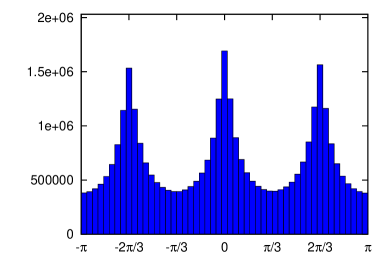
(a) $T<T_{C}$, approximately equal occupation

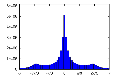
(b) $T>T_{C}$, there is a single dominant center phase

Figure 1: Histograms of the distribution of complex phases of local loops across a gauge field ensemble, showing differing occupation of the three center phases.

It has been observed [10, 9] that for SU(3) gauge theory below the critical temperature, the complex phase of the local Polyakov loops ($\phi(\vec{x})$ in $L(\vec{x})=\rho(\vec{x})\,e^{i\phi(\vec{x})}$) is distributed evenly between three peaks, one at each of the three center phases of SU(3) ($0$, $\frac{2\pi}{3}$, and $\frac{-2\pi}{3}$). We have seen a similar effect in our own simulations as shown in Fig. 1a. As the distribution of $L(\vec{x})$ is uniform about the three center phases, the expectation value $\left<L(\vec{x})\right>$ vanishes. Above the critical temperature, the center symmetry is spontaneously broken and one of the three peaks becomes dominant. We have replicated this in our simulations as shown in Fig. 1b. As a result, the expectation value $\left<L(\vec{x})\right>$ is non-zero.

2.2 Anisotropic Gauge Action

On the lattice, the temperature $T$ is related to the temporal extent $aN_{t}$ by $T=\frac{1}{aN_{t}}$. The volume $V=(aN_{s})^{3}$ depends on the spatial extent of the lattice $aN_{s}$. Most studies of center domains change the temperature by varying the lattice spacing [17, 9, 10, 11]. This is a problem because the volume of the lattice is changed as the temperature changes. The only way one can change the temperature of an isotropic lattice without changing the volume is by adding or removing lattice sites in the time direction. In order to be able to adjust the temperature in a continuous manner, we instead introduce anisotropy into the lattice, replacing the single lattice spacing $a$ with a spatial lattice spacing $a_{s}$ and a temporal lattice spacing $a_{t}$. In this way we can vary the temperature $T=\frac{1}{a_{t}N_{t}}$ while maintaining a constant volume $V=(a_{s}N_{s})^{3}$ by varying $a_{t}$ whilst holding $a_{s}$ fixed. This allows us to observe the evolution of the center clusters in gauge field configurations moving from a confined configuration to a deconfined configuration under the HMC algorithm with no change in physical volume. This cannot be done with any of the previous methods and is the first such presentation.

In order to introduce this anisotropy, we use the anisotropic Iwasaki action [18], which introduces an anisotropy parameter $\gamma_{G}$. This separates the Wilson loops in the plane of two spatial directions from the Wilson loops in the plane of a single spatial and temporal direction. The gauge action is

$$S_{G}[U] =\beta\Bigg{\{}\frac{1}{\gamma_{G}}\sum_{x,i>j}\left\{c_{0}^{s}P_{ij}(x)+c_{1}^{s}(R_{ij}(x)+R_{ji}(x))\right\}$$

$$+\gamma_{G}\sum_{x,k}\left\{c_{0}^{t}P_{k4}(x)+c_{1}^{t}R_{k4}(x)+c_{2}^{t}R_{4k}(x)\right\}\Bigg{\}}\,,$$

where $i$, $j$, $k$ are for spatial directions, and $P_{\mu\nu}(x)$ and $R_{\mu\nu}(x)$ are the $1\times 1$ plaquette and $1\times 2$ rectangular loop in the $\mu-\nu$ plane respectively, $\beta$ governs the strong coupling, $\gamma_{G}$ governs the anisotropy, and the improvement coefficients are [18]

$$c_{1}^{s}=c_{1}^{t}=c_{2}^{t} =-0.331$$

$$c_{0}^{s}=c_{0}^{t} =3.648\,.$$

2.3 Hybrid Monte-Carlo

We want to generate an ensemble of gauge field configurations $\left\{U_{i}\right\}$ with probability distribution $\rho(U)=e^{-S_{G}[U]}$. To do this, it is common to use local updates such as the pseudo heat-bath combined with over-relaxation algorithms as this is an efficient way to generate pure gauge field configurations. However, we are ultimately interested in dynamical fermion results, so we use the Hybrid Monte Carlo (HMC) algorithm [19]. This allows us to study the way the HMC algorithm evolves the gauge fields at fixed temperature and from a state thermalised at one temperature to a new state eventually thermalised at a higher temperature. This is of interest to the lattice community who use the HMC algorithm for generating dynamical gauge field ensembles, as it gives insight into the nature of the algorithm and correlation times.

The HMC algorithm involves introducing the non-physical constructs $\Pi_{\mu}$ and $\tau$, the conjugate momenta of $U$ and the simulation time respectively. We then describe the new extended system by the Hamiltonian

$$\mathcal{H}[U,\Pi]=\sum_{x,\mu}\frac{1}{2}\,\operatorname{Tr}\Pi_{\mu}(x)^{2}+S_{G}[U]\,.$$

To describe the frame rate of our visualisations, we briefly review the update algorithm. Starting from an initial gauge field configuration $U$, we apply the following process [20]:

1. Select a random $\Pi$ from an ensemble distributed according to $\rho(\Pi)\propto e^{-\frac{1}{2}\mathrm{Tr}\Pi^{2}}$

2. Perform molecular dynamics updates with step size $\Delta\tau$, evolving $U_{\mu}$ to to $U_{\mu}^{\prime}$ and $\Pi_{\mu}$ to $\Pi_{\mu}^{\prime}$ by the following discretised equations of motion (so that $\frac{d\mathcal{H}}{d\tau}\approx 0$):

   $$U_{\mu}(x,\tau+\Delta\tau)=U_{\mu}(x,\tau)\exp(i\Delta\tau\Pi_{\mu}(x,\tau))$$

   $$\Pi_{\mu}(x,\tau+\Delta\tau)=\Pi_{\mu}(x,\tau)-\Delta\tau U_{\mu}(x,\tau)\frac{\delta S_{G}}{\delta U_{\mu}(x,\tau)}$$

3. After $\frac{1}{\Delta\tau}$ updates, providing a trajectory length of 1, we accept or reject the new configuration with probability $\rho=\min(1,e^{-\Delta\mathcal{H}})$, where $\Delta\mathcal{H}=\mathcal{H}[U,\Pi]-\mathcal{H}[U^{\prime},\Pi^{\prime}]$.

In generating the configurations used in this paper, we used 150 molecular dynamics steps with step size $\Delta\tau=\frac{1}{150}$. When producing visualisations we store the state of the Polyakov loops five times per trajectory in order to make the animation smoother. Of course, these frames are dropped if the configuration is not accepted in step 3. The acceptance rates we observed when generating our gauge field configurations varied between 75% and 90%, depending on the volume and temperature of the configurations being generated. Large volumes and high temperatures have the lowest acceptance rates.

Independent gauge fields are saved every 50 trajectories, an order of magnitude more separation than the 5 trajectories often used in dynamical QCD.

As we will see, correlations in the centre clusters are associated with a time scale of 20 to 30 trajectories, or 4 to 6 seconds in the animations.

2.4 Lattice Spacings and Temperature

The lattice spacings $a_{s}$ and $a_{t}$ depend non-trivially on $\beta$ and $\gamma_{G}$. In order to determine $a_{s}$ and $a_{t}$ for a given $(\beta,\gamma_{G})$ pair, we perform a lattice simulation at zero temperature (high temporal extent) and fit the values of the Wilson loops, $W_{\mu\nu}(r,t)$, to the static quark potential

$$V(r)=V_{0}+\sigma r-e\cdot\left[\frac{1}{r}\right]+l\cdot\left(\left[\frac{1}{r}\right]-\frac{1}{r}\right)\,,$$

where $\left[\frac{1}{r}\right]$ denotes the tree-level lattice Coulomb term [21].

This ansatz for the static quark potential is sensitive to discretisation effects at extremely small $r$ and noise starts to dominate at large $r$, so we need a lower and upper cutoff for $r$.

On an anisotropic lattice, the fit for the space-space loops ($W_{xy}(r,t)$, $W_{xz}(r,t)$, and $W_{yz}(r,t)$) gives a string tension $\sigma_{ss}$ which is related to the spatial lattice spacing $a_{s}$ through the physical value $\sqrt{\sigma}=0.44\,\mathrm{GeV}$. On the other hand, the space-time loops, ($W_{xt}(r,t)$, $W_{yt}(r,t)$, and $W_{zt}(r,t)$) and the time-space loops ($W_{tx}(r,t)$, $W_{ty}(r,t)$, and $W_{tz}(r,t)$) give $\sigma_{st}$, which is related to both the spatial and temporal lattice spacings via $\sqrt{a_{s}a_{t}}$.

Table 1: The $(\beta,\gamma_{G})$ pairs obtained from pure gauge simulations of $24^{3}\times 48$ lattices and the corresponding temperatures for a $24^{3}\times 8$ lattice.

$\beta$	$\gamma_{G}$	$a_{s}$ (fm)	$a_{t}$ (fm)	$\xi$	$T$ (MeV)
2.620	1.000	0.1016(5)	0.1028(11)	0.988(12)	240(3)
2.645	1.125	0.1014(4)	0.0912(8)	1.112(12)	270(2)
2.670	1.250	0.1019(6)	0.0803(10)	1.245(19)	307(4)
2.695	1.375	0.1014(4)	0.0761(8)	1.335(25)	324(3)
2.720	1.500	0.1002(9)	0.0673(10)	1.489(31)	366(5)
2.740	1.625	0.1007(12)	0.0622(8)	1.618(39)	396(5)
2.760	1.750	0.1019(8)	0.0567(9)	1.796(38)	434(7)

By finding $a_{s}$ and $a_{t}$ for a variety of $(\beta,\gamma_{G})$ pairs, the relationship between $\beta$ and $\gamma_{G}$ necessary to keep $a_{s}$ constant can be determined. This allows us to choose a set of $(\beta,\gamma_{G})$ pairs that give us access to a range of temperatures at a fixed volume as shown in Table 1.

We also found that the renormalised anisotropy,

$$\xi=\frac{a_{s}}{a_{t}}\,,$$

is approximately equal to the bare anisotropy, $\gamma_{G}$, in the region we studied.

2.5 Potts Model

The universal properties at finite temperature phase transitions in (3 + 1) dimensional gauge theories are related to those in 3-dimensional spin models [22, 16]. Thus, it is of interest to compare the behavior of the Polyakov loops in QCD with the three dimensional 3-state Potts model [23], a generalisation of the Ising spin model. In the 3-state Potts model, each lattice site can assume one of three spin directions and these form spin aligned domains. After the phase transition, one direction dominates the space, just as in the QCD deconfinement transition. Thus, the Potts model is a candidate for a simplified model of deconfinement.

The 3-state Potts model for a three dimensional lattice of points $\vec{x}\in\mathbb{L}\subset\mathbb{Z}^{3}$ with spin $\sigma(\vec{x})=1,2\text{ or }3$ at each lattice site is described by the partition function

$$Z=e^{-\beta E[\sigma]}\,,$$

where

$$E[\sigma]=\sum_{\vec{x}}\sum_{i}\delta_{\sigma(\vec{x}),\sigma(\vec{x}+\hat{\imath})}\,,$$

is summed over the points of the lattice and the three spatial directions, $\hat{\imath}$ is the unit vector in the positive $i$ direction, and $\delta_{j,k}$ is the Kronecker delta. That is, $E[\sigma]$ is the total number of spin-aligned nearest-neighbor pairs. Here, $\beta=J/k_{B}T$ is the inverse temperature in natural units.

We can simulate this using the Metropolis-Hastings algorithm [24] to study the behavior of spin-aligned domains near the critical temperature and compare it to the behavior of center clusters in QCD near $T_{C}$.

3 Results

3.1 Visualisation

In order to analyse the behavior of the Polyakov loops at the critical temperature, we generate gauge field configurations on several $24^{3}\times 8$ lattices with the same spatial lattice spacing but different temporal spacings, using the parameters described in Section 2.

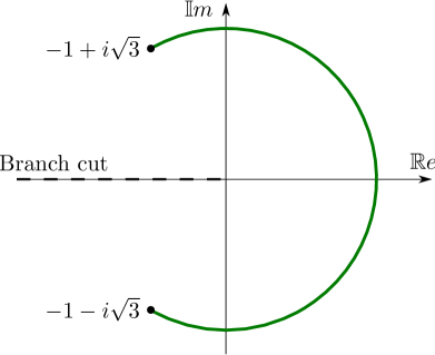
(a) Interpolation of phase

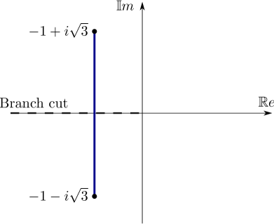
(b) Interpolation of complex value

Figure 2: Diagrams showing path followed by different interpolation methods.

(a) Interpolation of phase (artifacts)

(b) Interpolation of complex value

Figure 3: Visualisations demonstrating the (red) artifacts produced by the incorrect phase interpolation on the left. On the right, the correct complex interpolation shows an equal center phase distribution.

Visualising the Polyakov loop data presents a difficulty. Most visualisation software that has the ability to render volumetric data takes in a three dimensional grid of real values and uses trilinear interpolation to fill in the gaps. However, if we try to do this with the complex phase of our Polyakov loop values (with a branch cut at $\pi$), we find that the interpolation has problems near the branch cut. For example, if two adjacent data points have complex values $-1\pm i\sqrt{3}$ (corresponding to complex phases of $\phi=\frac{\pm 2\pi}{3}$) then interpolating the phase linearly between the two points takes it through $\phi=0$ as in Fig. 2a, rather than crossing the branch cut as in Fig. 2b. This behavior is incorrect and produces artifacts in the final image that look like thin shells or films between regions of transparency. This leads to much more red (corresponding to $\phi=0$) than either of green or blue ($\phi=\frac{2\pi}{3}$ and $\phi=\frac{-2\pi}{3}$ respectively) as seen in Fig. 3a.

Instead, we want to directly interpolate the complex numbers and then calculate the phase, resulting in the phase going directly between the two endpoints, across the branch cut as in Fig. 2b. This results in a significantly different visualisation as seen in Fig. 3b.

To circumvent this problem, we have developed a custom volume renderer for complex valued scalar fields. The details of the rendering algorithm are given in A. There we present two ways of visualising the center clusters, one based on proximity of $\phi(\vec{x})$ to one of the three center phases and one on the magnitude $\rho(\vec{x})$.

3.2 Critical Temperature

Four animations are available online at the URL provided in Ref. [25]. This is the first presentation of animations of the evolution of center clusters under the HMC algorithm. Two different rendering techniques are presented. As discussed in A, these include rendering based on the proximity of $\phi(\vec{x})$ to one of the three center phases of SU(3) and rendering based on the magnitude $\rho(\vec{x})$. Each are rendered from the original configurations as well as configurations smoothed with four sweeps of stout-link smearing as discussed in greater detail below.

(a)

(b)

Figure 4: Histogram of the phase $\phi(\vec{x})$ and a visualisation of the center clusters in the local Polyakov loop values at $T=0.89(1)\,T_{C}$. All three center phases are present in small clusters with approximately equal density.

The animations reveal the evolution of center clusters as a function of the HMC simulation time, with five frames per unit trajectory. The evolution of the center clusters is governed by the evolution of the gauge field configurations under the HMC algorithm, and therefore the timescale of these animations is not a physical scale but an algorithmic scale. However, while it may have no direct physical significance, the evolution of the center clusters during thermalisation gives novel insights into the nature of the HMC algorithm and the way it brings the gauge field to a physical configuration. In addition, once thermalisation is complete, every frame in itself is a physically representative state and thus we can observe a number of possible structures for the center clusters and gain extensive insight.

We commence with a thermalised configuration at $T=240(3)\,\mathrm{MeV}$ or $T/T_{C}=0.89(1)$. We select a $24^{3}$ spatial volume and note that it is representative of the other volumes considered herein. To show the nature of the HMC updates, we present 750 frames corresponding to 150 HMC trajectories. At our framerate of 25 frames per second, this lasts 30 seconds. A snapshot of the center clusters at this temperature is provided in Fig. 4. On the left-hand plot, a histogram of the distribution of the phases of the Polyakov loops across a gauge field ensemble at this temperature shows that all three center phases, observable as peaks in the histogram, are approximately equally occupied, signaling confinement. The right-hand plot shows a single frame from the animation, in which the three center-phase peaks observed in the histogram correspond to blue (left), red (center), and green (right). All three center phases are present in small clusters with approximately equal density.

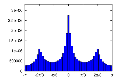
(a)

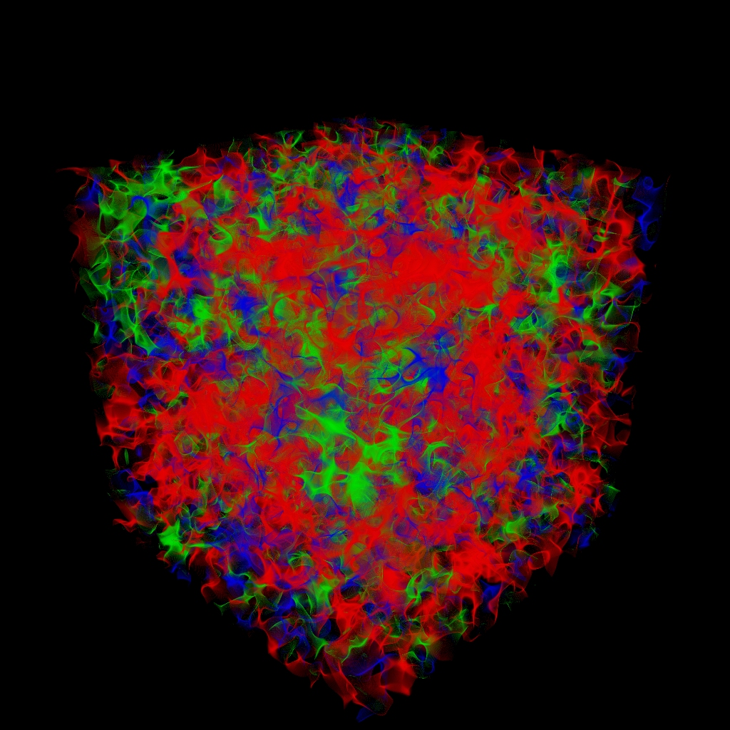
(b)

Figure 5: Histogram and visualisation as in Fig. 4 at $T=1.14(2)\,T_{C}$. A single(red) phase is beginning to dominate, signaling deconfinement.

At this point (0:30 in the animation), the temperature is increased to $T=307(4)\,\mathrm{MeV}$ or $T/T_{C}=1.14(2)$ and the response of the gauge field is illustrated in the animations. Fig. 5 shows the red center phase becoming dominant with the other two beginning to be suppressed, signaling the onset of deconfinement. In the animation, we can see that the three center phases start out equally dominant and fluctuate in size until the red clusters come to dominate.

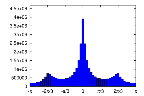
(a)

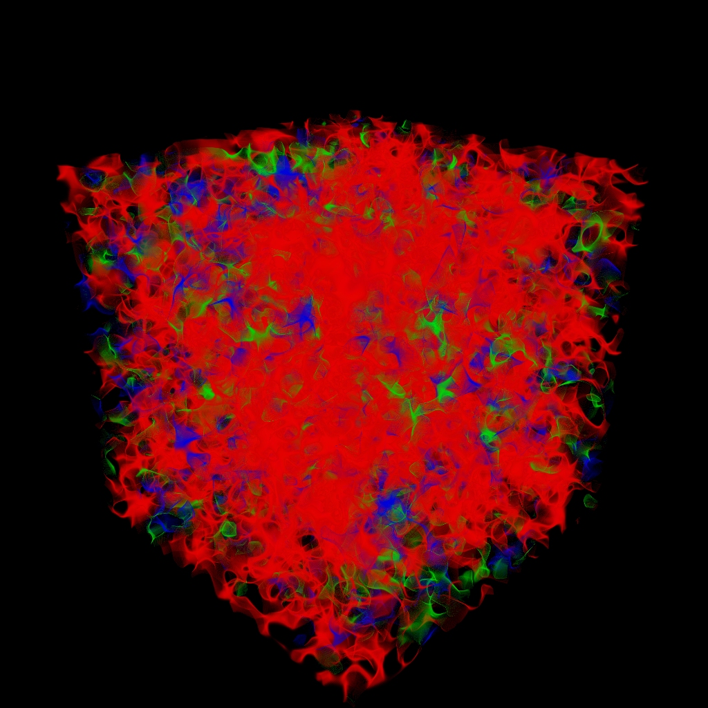
(b)

Figure 6: Histogram and visualisation at $T=1.36(2)\,T_{C}$. A single (red) cluster dominates the entire space.

After 600 HMC trajectories or 120 seconds, at 2:30 in the animation, the configuration has responded to the temperature change and we increase the temperature again, this time to $T=366(5)\,\mathrm{MeV}$ or $T/T_{C}=1.36(2)$. At this temperature, the animation shows that the red clusters continue to grow, occupying almost the entire space. This can be seen in the snapshot provided in Fig. 6.

(a)

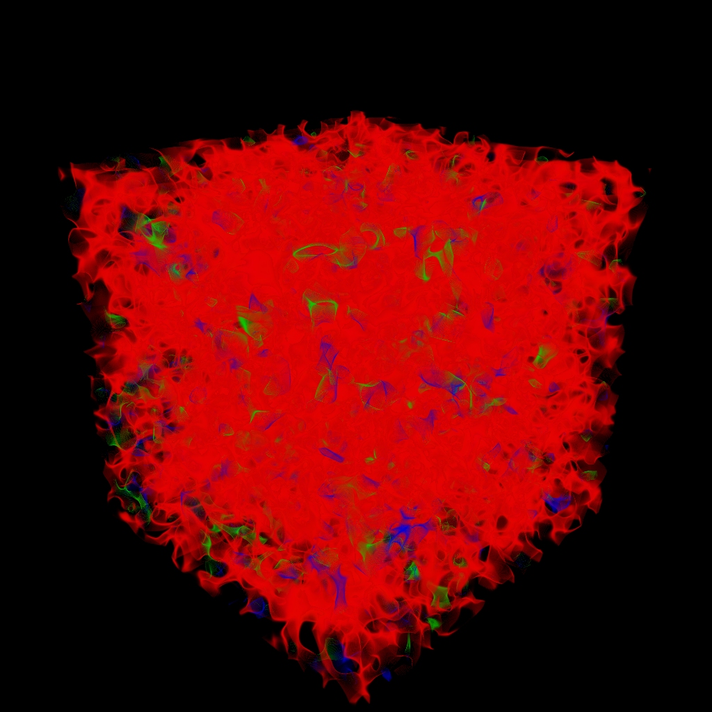
(b)

Figure 7: Histogram and visualisation at $T=1.61(3)\,T_{C}$. The same (red) phase is still dominant.

After 250 more HMC trajectories or 50 seconds, at 3:20 in the animation, we increase the temperature again, to $T=434(7)\,\mathrm{MeV}$ or $T/T_{C}=1.61(3)$. At this temperature, the red phase remains dominant in the animation and the other two phases are suppressed even further. Fig. 7 provides a snapshot at this temperature, showing the red phase almost completely dominant. We show 250 HMC trajectories at this temperature over the remaining 50 seconds of the animation.

3.3 Monte-Carlo Evolution

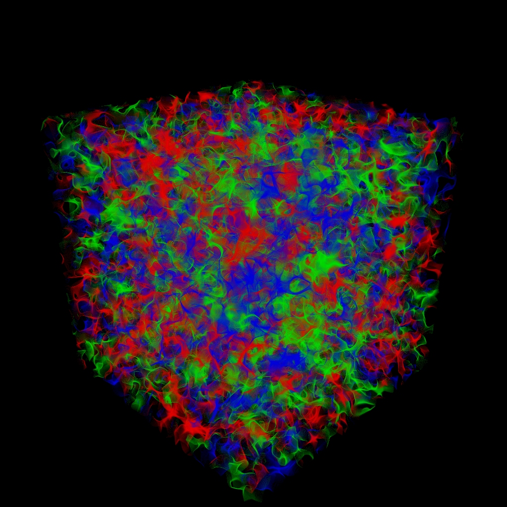
(a) Thermalised configuration

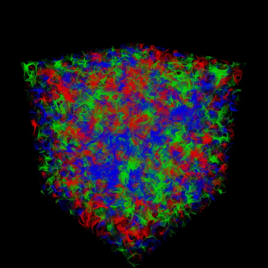
(b) After one unit HMC trajectory

Figure 8: Evolution of center clusters with simulation time at $T=0.89(1)\,T_{C}$.

By examining visualisations of the center clusters on gauge field configurations separated by a single HMC trajectory, we can observe the evolution of the center clusters with simulation time. The autocorrelation times for different observables under HMC evolution can vary, so it is of interest to observe the timescales over which the center clusters evolve. We can see that over the course of a single unit trajectory, the small scale structure of the loops changes significantly, as shown in Fig. 8. This suggests that the small scale structure of the center clusters evolves very quickly under the HMC algorithm and thus has short autocorrelation times.

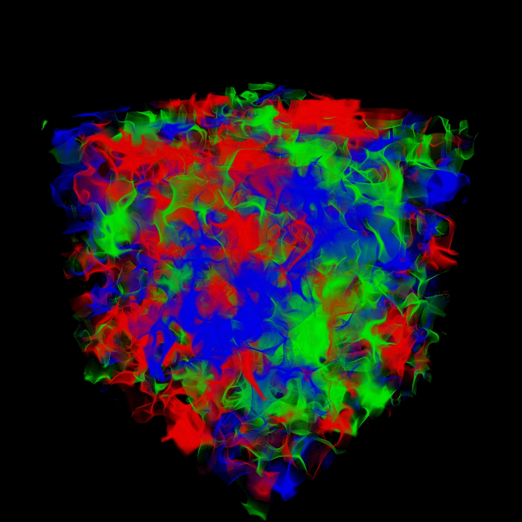
(a) Thermalised configuration

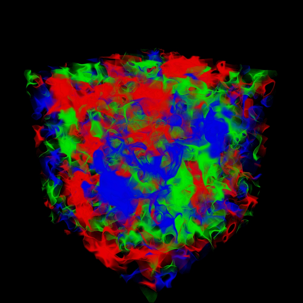
(b) After one unit HMC trajectory

Figure 9: Evolution of center clusters with simulation time at $T=0.89(1)\,T_{C}$. Four sweeps of stout-link smearing are applied to the gauge links prior to calculating the Polyakov loops.

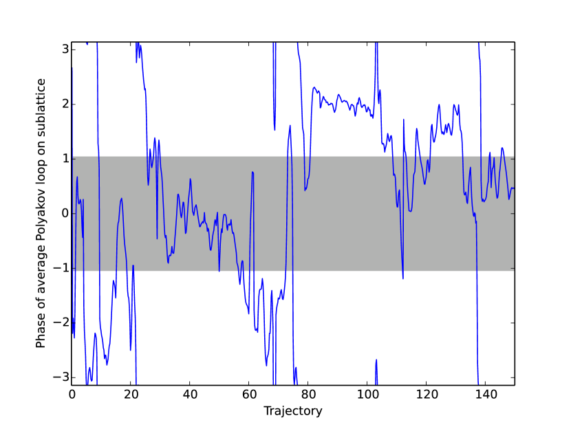
Figure 10: Evolution of phase of average Polyakov loop on $6\times 6\times 6$ sublattice with simulation time at $T=0.89(1)\,T_{C}$. Four sweeps of stout-link smearing are applied to the gauge links prior to calculating the Polyakov loops. Since the phase is $2\pi$-periodic, we see the graph wrapping around on the y-axis.

To investigate the larger scale behavior of the clusters, we remove the small scale noise by performing four sweeps of stout-link smearing [26] prior to calculating the Polyakov loops. The results are illustrated in Fig. 9. In these visualisations, we see that over the course of one trajectory, the center clusters are slowly moving, with some change around the boundaries of the clusters. Observing the evolution of the center clusters in the corresponding animation, we see correlations in the center clusters persisting for approximately 5 seconds corresponding to 25 trajectories, suggesting an approximate length for the autocorrelation time of the larger scale structure of the clusters. After approximately 50 trajectories, the large scale structure of the loops has become completely decorrelated. This is supported by Fig. 10, which shows the phase of the average Polyakov loop on a small ($6\times 6\times 6$) subsection of the lattice. We can see that the phase becomes completely decorrelated within 50 trajectories. This supports our choice of separation for independent configurations.

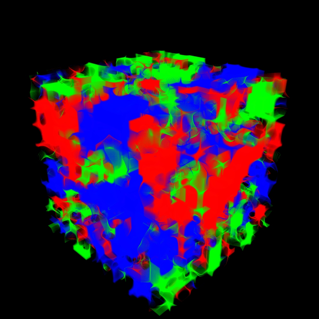
(a) Thermalised configuration

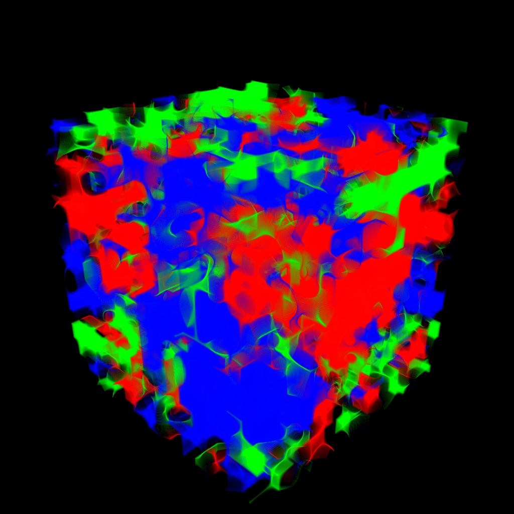
(b) After 4096 single-site Metropolis updates

Figure 11: Evolution of spin-aligned domains in the three dimensional 3-state Potts model at $\beta=0.55$ on a $16^{3}$ lattice.

The evolution observed in $SU(3)$ gauge theory is consistent with the behavior of spin-aligned domains in the three dimensional 3-state Potts model [23] just below the critical temperature under Metropolis-Hastings algorithm simulations, as seen in Fig. 11.

We can also see that once a particular center phase comes to dominate the space, that phase remains dominant for the rest of the simulation. That is, in this first investigation of the behaviour of the Polyakov loop under Monte-Carlo evolution, we find that the dominant phase is highly stable under the process of HMC updates.

3.4 Magnitude-Based Clusters

(a) Opacity based on $\phi(\vec{x})$

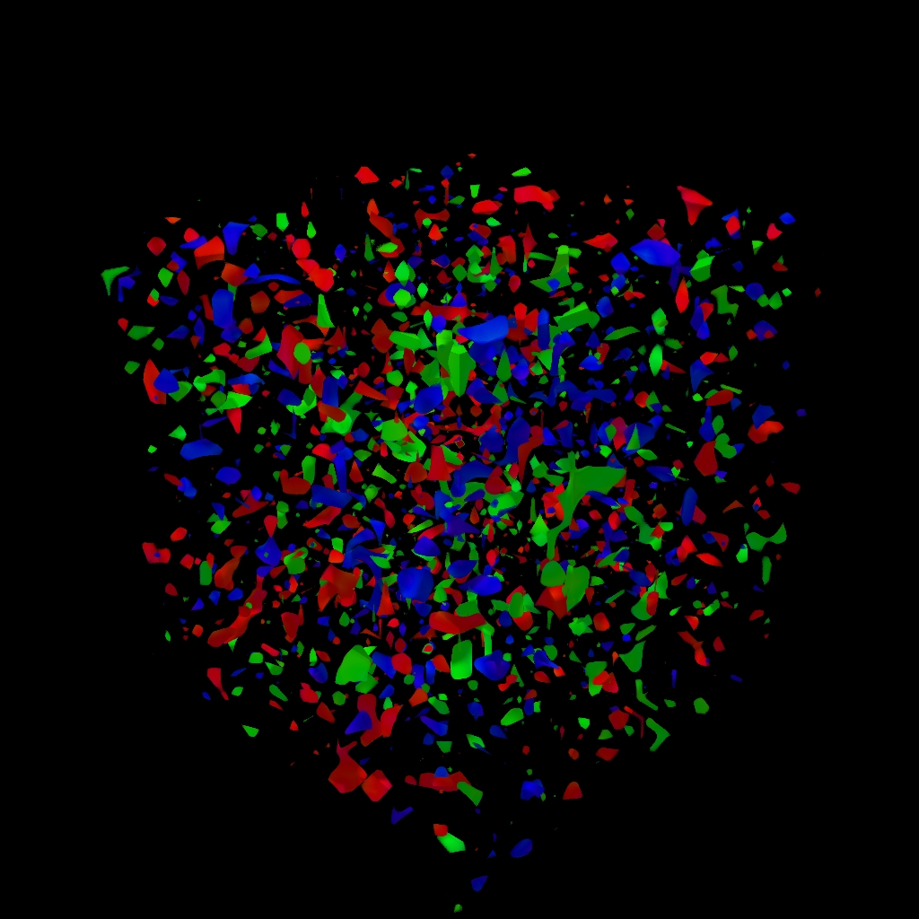
(b) Opacity based on $\rho(\vec{x})$

Figure 12: Comparison of complex phase $\phi(\vec{x})$ and magnitude $\rho(\vec{x})$ clusters at $T=0.89(1)\,T_{C}$.

If we use the alternate rendering style based on the magnitude $\rho(x)$, we can see that peaks in the magnitude lie approximately within the center clusters, as shown in Fig. 12. The magnitude peaks are each colored corresponding to a single center phase and they appear to line up with peaks in the corresponding phase based visualisation. However it is not necessarily clear that each center cluster corresponds to a peak in the modulus, $\rho(\vec{x})$.

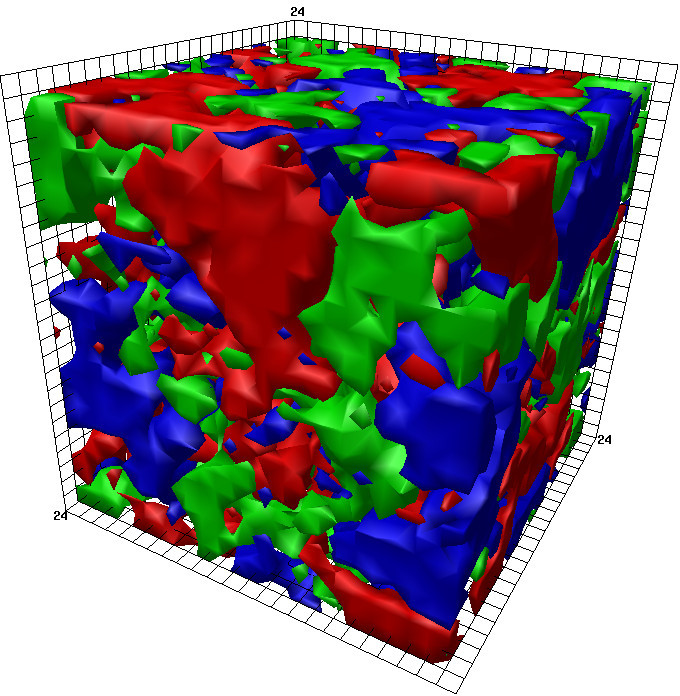
(a) Clusters based on $\phi(\vec{x})$

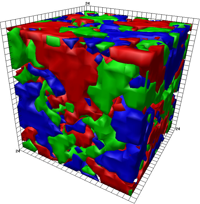
(b) Clusters based on $\rho(\vec{x})$

Figure 13: Comparison of phase $\phi(\vec{x})$ and magnitude $\rho(\vec{x})$ clusters at $T=0.89(1)\,T_{C}$ after four sweeps of stout-link smearing using the isovolume renderer. The rendering thresholds for $\phi(\vec{x})$ and $\rho(\vec{x})$ are 0.5 and 0.2 respectively.

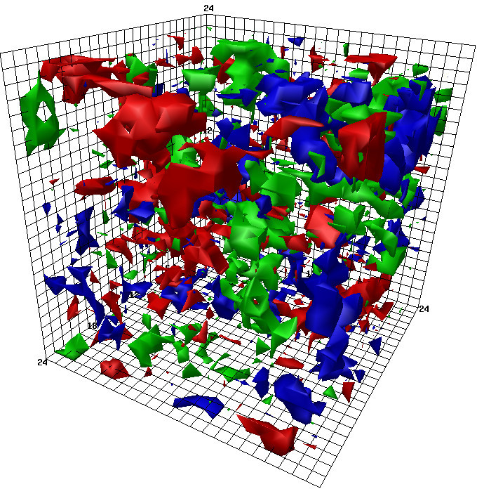
(a) Clusters based on $\phi(\vec{x})$

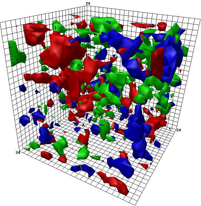
(b) Clusters based on $\rho(\vec{x})$

Figure 14: Comparison of phase $\phi(\vec{x})$ and magnitude $\rho(\vec{x})$ clusters at $T=0.89(1)\,T_{C}$ after four sweeps of stout-link smearing, using the isovolume renderer, cut much closer into the peaks than Fig. 13. Here, the rendering thresholds for $\phi(\vec{x})$ and $\rho(\vec{x})$ are 0.9 and 0.5 respectively.

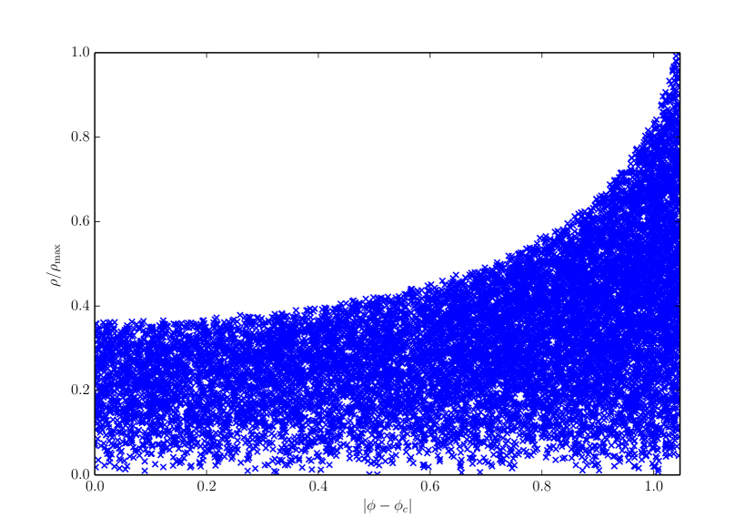
Figure 15: Scatter plot of center phase proximity and modulus, showing a clear correlation between proximity to a center phase and maxima of the modulus.

In order to look more closely at the correlation between these clusters, we again perform four sweeps of stout-link smearing, making it easier to observe larger scale structures, and render both the phase and magnitude based clusters using an isovolume rendering developed in AVS/Express [27] that makes the boundaries of the clusters more clear. When we do this, it becomes clear that there is an approximate one-to-one relationship between the peaks in the magnitude $\rho(\vec{x})$ and the proximity of $\phi(\vec{x})$ to a center phase. The measures $|\phi(\vec{x})-\phi_{c}(\vec{x})|/(\pi/3)$ and $\rho(x)/\rho_{\mathrm{max}}$ are illustrated in Figs. 13 and 14. We can also observe this correlation by looking at a scatter plot of $\rho(x)/\rho_{\mathrm{max}}$ vs $|\phi(\vec{x})-\phi_{c}(\vec{x})|$ as in Fig. 15. This observed correlation of $\rho(\vec{x})$ becoming small as $\phi(\vec{x})$ moves away from a center phase is the first direct confirmation of the underlying assumption of Ref. [5], which links the center domain walls to unanticipated phenomena observed at RHIC [28] and the LHC [6, 7, 8].

These peaks in the magnitude of the local Polyakov loops mean that the free energy of a quark-antiquark pair is minimised in the core of a center cluster. Thus we have a confining potential with local minima at the cores of center clusters. Below the critical temperature the peaks are sharp so the gradient of the potential is steep, resulting in a strong restoring force confining the quarks to the core of the cluster. Above the critical temperature, the peaks become much broader so the gradient is significantly smaller and the restoring force is greatly reduced.

3.5 Center Clusters

The local Polyakov loop $L(\vec{x})$ is a complex number at each spatial lattice site $\vec{x}$. We can express it in complex polar form,

$$L(\vec{x})=\rho(\vec{x})\,e^{i\phi(\vec{x})}\,,$$

where $\rho(\vec{x}),\phi(\vec{x})\in\mathbb{R}$, $\rho(\vec{x})\geq 0$, and $-\pi<\phi(\vec{x})\leq\pi$.

In order to observe the structure of individual clusters, we use the definition by Gattringer and Schmidt [9]. Two neighboring points $\vec{x}$ and $\vec{y}$ belong to the same cluster iff $n(\vec{x})=n(\vec{y})$, where the sector number $n(\vec{x})$ is defined to be

$$n(\vec{x}):=\left\{\begin{array}[]{lr}-1&\mathrm{for}\,\phi(\vec{x})\in[-\pi+\delta,-\frac{\pi}{3}-\delta],\\ 0&\mathrm{for}\,\phi(\vec{x})\in[-\frac{\pi}{3}+\delta,\frac{\pi}{3}-\delta],\\ 1&\mathrm{for}\,\phi(\vec{x})\in[\frac{\pi}{3}+\delta,\pi-\delta].\end{array}\right.$$

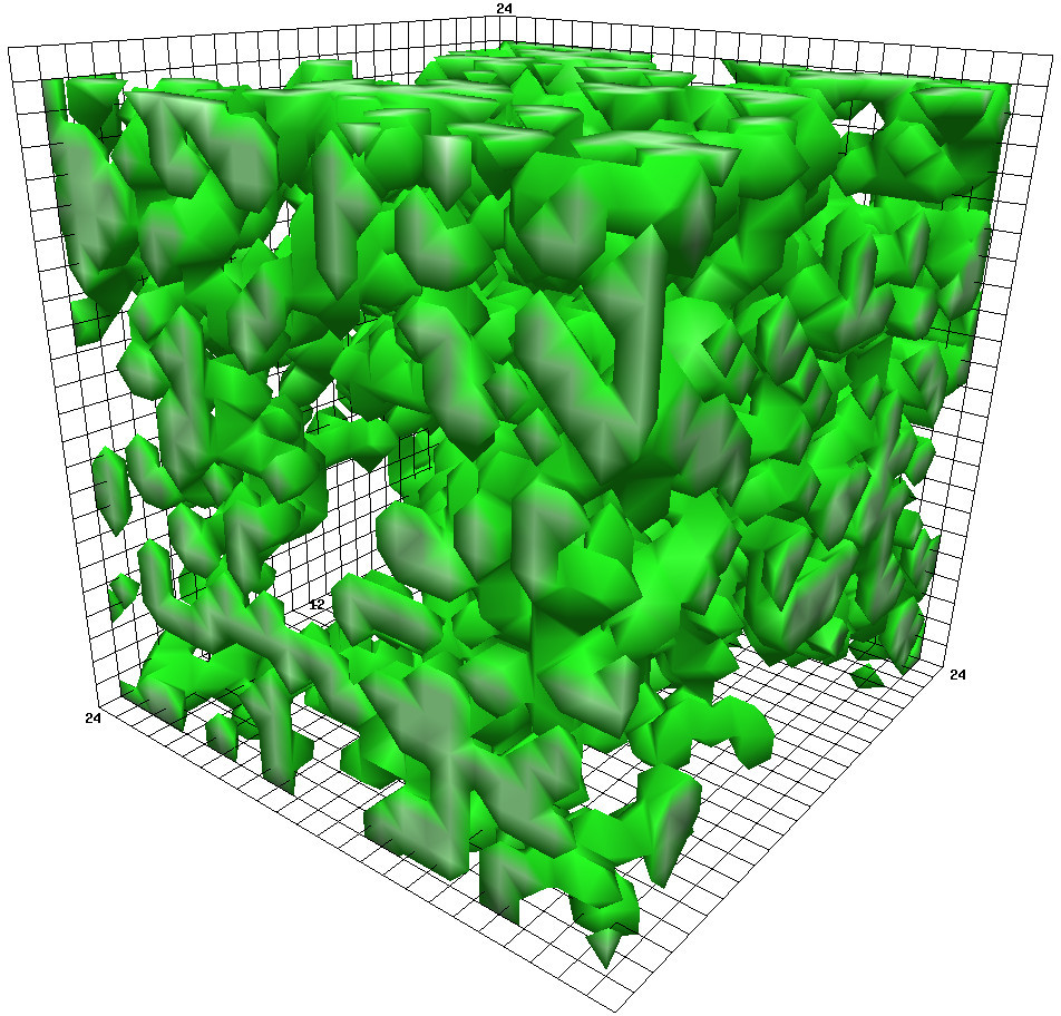
(a)

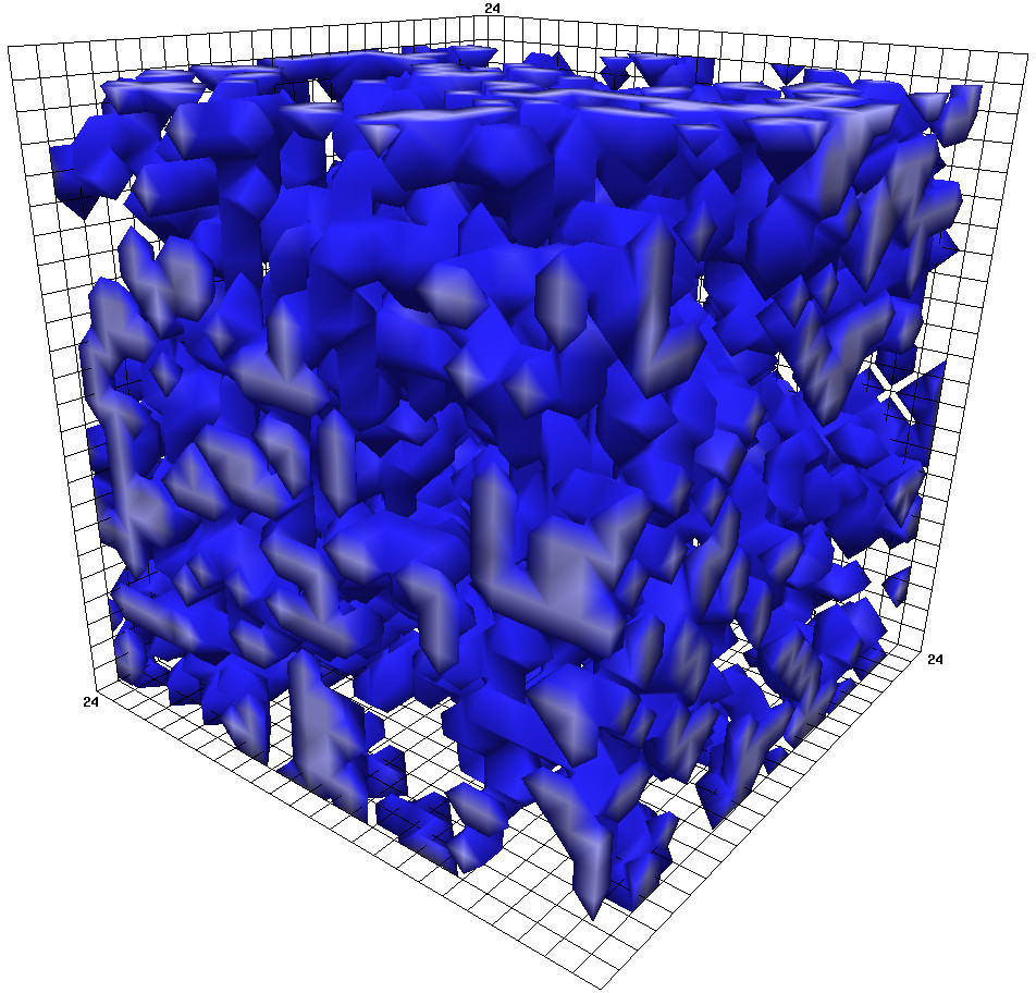
(b)

Figure 16: Two of the three percolating clusters in a representative $24^{3}\times 8$ gauge field configuration at $T=0.89(1)\,T_{C}$ when using a cut parameter of zero.

If we include every site in a cluster (i.e. we set the cut parameter $\delta$ to zero), then below the critical temperature each sector is equally occupied so our clustering is comparable to random site percolation theory with an occupation probability of $p\approx 0.3333$. This is above the critical percolation probability of $p_{c}=0.3116$ [29]. Thus, with a cut parameter of zero, we expect to see at least one percolating cluster (i.e. a cluster that has at least one site in each of the $3N_{s}$ spatial planes) for each phase. Thus, if we define the clusters in this way, due to the nature of three dimensional space they are not localized, and instead extend over the entire lattice, as seen in Fig. 16.

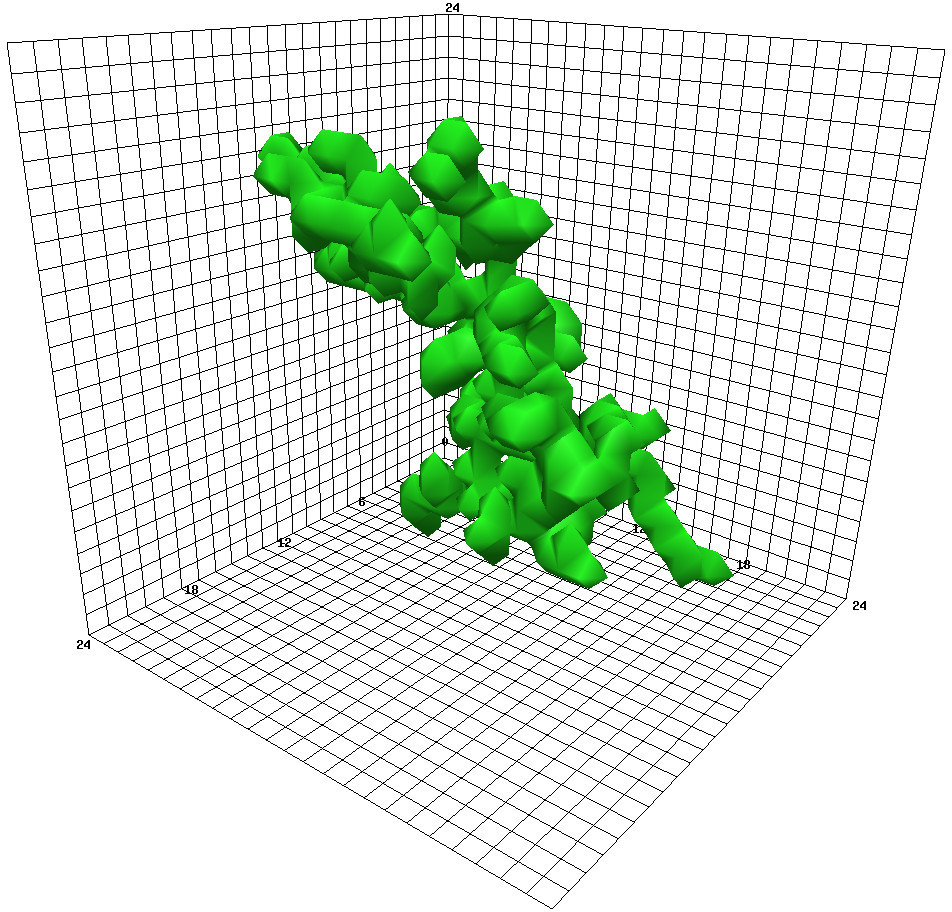
(a)

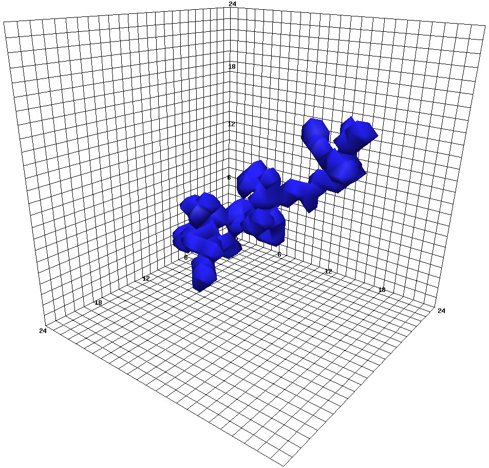
(b)

Figure 17: One of the non-percolating clusters broken off from each of the clusters in Fig. 16 when the cut parameter is increased to 0.3.

In order to study localized clusters below the critical temperature, we instead introduce a cut parameter as in Ref. [9]. This results in smaller, localized clusters scattered across the lattice. Fig. 17 illustrates results for $\delta=0.3$. We can see that these clusters have a one dimensional, finger-like quality to their structure and this supports the determination by Endrodi, Gattringer and Schadler [13] that the center clusters have a fractal dimension of $D\approx 1.4-1.7$.

As illustrated in Fig.15, the selection of a cut in $\phi(\vec{x})$ identifies a subset of points where $\rho(\vec{x})$ is small and attributes the points to a domain wall of finite thickness.

Just as the expectation value of $L$ is related to the free energy of a static quark relative to the vacuum by

$$\left<L(\vec{x})\right>\propto\exp(-F_{q}/T)\,,$$

the correlation function $\left<L(\vec{x})L(\vec{y})^{\dagger}\right>$ is related to the free energy of a static quark-antiquark pair (a meson) separated by $\vec{x}-\vec{y}$ [16]:

$$\left<L(\vec{x})L(\vec{y})^{\dagger}\right>\propto\exp(-F_{q\bar{q}}(\vec{x}-\vec{y})/T)\,.$$

Thus:

1. If $\left<L(\vec{x})L(\vec{y})^{\dagger}\right>\neq 0$, then $F_{q\bar{q}}(\vec{x}-\vec{y})$ is finite.

2. If $\left<L(\vec{x})L(\vec{y})^{\dagger}\right>=0$, then $F_{q\bar{q}}(\vec{x}-\vec{y})$ is infinite.

If we consider these smaller, localized center clusters, we can then conclude the following:

1. If $\vec{x}$ and $\vec{y}$ lie within a single cluster, $\phi(\vec{x})\approx\phi(\vec{y})$ and

   $$\left<L(\vec{x})L(\vec{y})^{\dagger}\right> =\left<\rho(\vec{x})\rho(\vec{y})e^{i(\phi\left(\vec{x})-\phi(\vec{y})\right)}\right>$$

   $$\approx\left<\rho(\vec{x})\rho(\vec{y})\right>$$

   $$\neq 0\,.$$

   That is, the phases at $\vec{x}$ and $\vec{y}$ cancel out, and the correlation function is non-zero. Thus, $F_{q\bar{q}}(\vec{x}-\vec{y})$ is finite and quark-antiquark pairs can be separated within a cluster.

2. If $\vec{x}$ and $\vec{y}$ lie within different clusters, $\phi(\vec{x})\neq\phi(\vec{y})$ in general and thus there is no correlation between the phases. Due to the symmetry of the distribution of the phases between clusters, the three center phases are equally present. Across an ensemble they average to zero, giving

   $$\left<L(\vec{x})L(\vec{y})^{\dagger}\right> =0$$

   Thus, $F_{q\bar{q}}(\vec{x}-\vec{y})$ is infinite and quark-antiquark pairs cannot be separated across cluster boundaries.

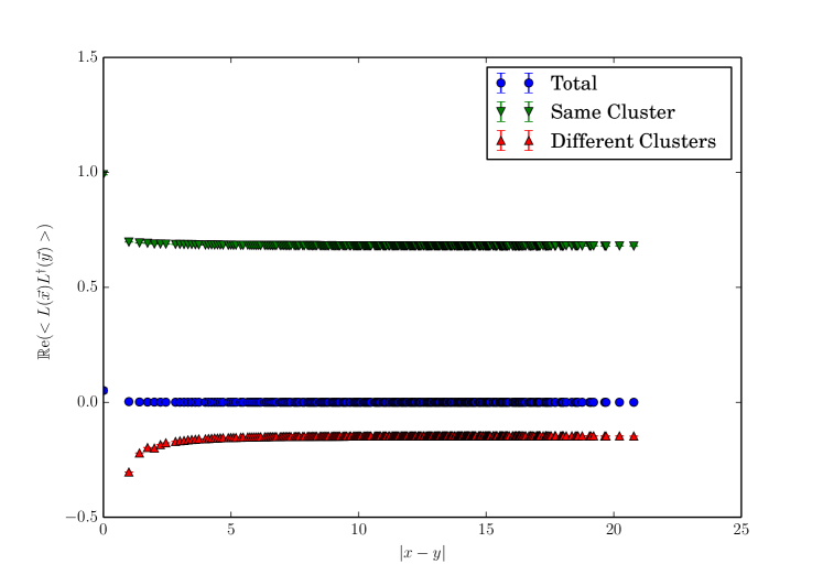
Figure 18: Comparison of real component of correlation function for points in the same and in different clusters and averaged across all points. Generated from $24^{3}\times 8$ lattice at $T=0.89(1)\,T_{C}$ with a cut parameter of $0.0$.

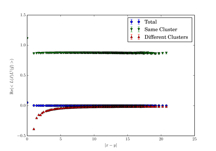
Figure 19: Comparison of real component of correlation function for points in the same and in different clusters and averaged across all points. Generated from $24^{3}\times 8$ lattice at $T=0.89(1)\,T_{C}$ with a cut parameter of $0.3$.

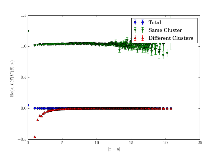
Figure 20: Comparison of real component of correlation function for points in the same and in different clusters and averaged across all points. Generated from $24^{3}\times 8$ lattice at $T=0.89(1)\,T_{C}$ with a cut parameter of $0.5$.

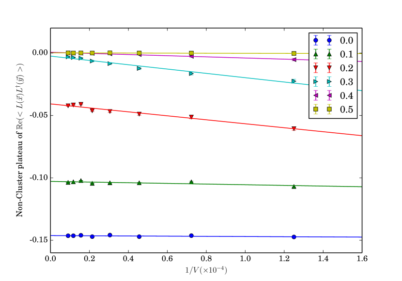
Figure 21: Volume and cut parameter dependence of the plateau in the correlation function for different clusters at $T=0.89(1)\,T_{C}$. Cut parameters are indicated in the legend.

We can observe that this is approximately the case for sufficiently large $\left|\vec{x}-\vec{y}\right|$ in Figs. 18-20, produced from an ensemble of 100 independent gauge field configurations, which show that the real component of the correlator is nonzero and positive for points in the same cluster and plateaus to a small negative value for points in different clusters. The imaginary component is negligible. As can be seen from Fig. 21, the nonzero negative value of the plateau is a finite volume effect that goes to zero in the infinite volume limit for sufficiently large values of the cut parameter. This effect results from the cluster at one point (say $\vec{x}$) extending to the neighborhood of $\vec{y}$ and disturbing the even distribution of clusters between the three phases. In order for the correlation function to vanish, we need a cut parameter that is sufficiently large that the clusters have a finite size and a volume significantly larger than that size. This allows us to access an even distribution between the three phases so that it can average to zero.

Thus, the cluster size has a physical significance, governing the confining scale of the theory and the size of mesons. Below the critical temperature, when (given a sufficiently large cut parameter), the clusters have a limited finite size, this results in confinement. From a model perspective, this scale governs the size of the quark core of hadrons which is dressed by the mesonic cloud. Above the critical temperature, as a single cluster grows to encompass the entire space (regardless of the cut used), the quarks become deconfined [9].

4 Conclusion

We simulated SU(3) Yang-Mills theory on anisotropic $24^{3}\times 8$ lattices with the Iwasaki gauge action, considering renormalised anisotropy ranging from $\xi\approx 0.99$ to $\xi\approx 1.80$ with a spatial lattice spacing of $a_{s}\approx 0.1$. We explored temperatures ranging from $0.89(1)\,T_{C}$ to $1.61(3)\,T_{C}$. Our focus is on the structure and evolution of center clusters associated with Polyakov loops.

In doing so, we developed a volume rendering program that correctly deals with the interpolation of three dimensional complex fields such as the local Polyakov loop, and clearly displays their phase (and/or absolute value). This allows us to observe the evolution of center clusters with HMC simulation time.

For the first time, we were able to reveal the evolution of center clusters as they transitioned from the confined to the deconfined phase. The cluster behavior is consistent with that of spin aligned domains in the three dimensional 3-state Potts model. This supports the idea that the phase transition in QCD is comparable to that of a three state spin system.

We also observe an approximate one to one correspondence between peaks in the magnitude of local Polyakov loops and the locations of center clusters defined by the proximity of the phase of the Polyakov loops to a center phase. Gaps between the clusters illustrate the magnitude of the Polyakov loop is suppressed within the domain walls. This observation supports the underlying assumption of Ref. [5], linking the center domain walls to phenomena observed at RHIC [28] and the LHC [6, 7, 8].

The creation of a domain wall of finite thickness between clusters through the cut parameter $\delta$ [9] produces clusters in which the quark-antiquark correlation function $\left<L(\vec{x})L^{\dagger}(\vec{y})\right>$ vanishes when both quarks do not reside in the same cluster, setting a scale for confinement.

These peaks in the magnitude are sharp below the critical temperature. Through considerations of the free energy of multi-quark systems, this results in a minimum of the quark-antiquark potential in the core of each center cluster with a steep gradient resulting in a strong restoring force confining the quarks within the cluster. Above the critical temperature the peak structure becomes smooth and the region covered by the domain becomes large. When averaged over an ensemble, any remaining fluctuations in the Polyakov loops are smoothed out and the restoring force becomes negligible. In this way, quarks become deconfined.

Appendix A Visualisation

A.1 Algorithm

In order to perform the visualisation, we use a ray-traced volume renderer. For each pixel in the final image, a single ray is traced out directly away from the viewer through the volume to be rendered, accruing color and opacity based on the volumetric data.

Given a RGB (red, green, blue) color vector $C^{vol}(\vec{x})$ and an opacity $\alpha^{vol}(\vec{x})$ at every point $\vec{x}$ in the volume, we accrue color and opacity along a ray $\vec{x}(z)$ ($0\leq z\leq 1$, where $\vec{x}(0)$ is the point where the ray enters the volume and $\vec{x}(1)$ the point where it exits) by the differential equations,

$$\frac{d\alpha^{ray}(z)}{dz} =\left(1-\alpha^{ray}(z)\right)\alpha^{vol}\left(\vec{x}(z)\right)\,,$$

$$\frac{dC^{ray}(z)}{dz} =\left(1-\alpha^{ray}(z)\right)C^{vol}\left(\vec{x}(z)\right)\,.$$

To solve these differential equations, we use Euler’s method, with a finite step size $\Delta z$ [30]:

$$\alpha^{ray}_{n+1} =\alpha^{ray}_{n}+\Delta z\left(1-\alpha^{ray}_{n}\right)\alpha^{vol}\left(\vec{x}(z_{n})\right)\,,$$

$$C^{ray}_{n+1} =C^{ray}_{n}+\Delta z\left(1-\alpha^{ray}_{n}\right)C^{vol}\left(\vec{x}(z_{n})\right)\,.$$

In order to perform these calculations, we use OpenGL [31], a 2D and 3D graphics API that allows us to leverage the powerful hardware available in modern GPUs which is designed specifically for rendering graphics. OpenGL provides a flexible graphics processing pipeline which for our purposes consists of a vertex shader followed by a fragment shader. The vertex shader takes in information about the position and shape of three dimensional objects to be rendered and transforms them into the two dimensional space of the screen. The fragment shader runs once for each pixel on the screen, taking information about the polygon visible at that point from the vertex shader and determining the color the pixel should be.

In our particular case, we adapt a technique by Kruger and Westermann [32] which involves repeatedly rendering a single cube with a sequence of different shader pairs. The vertex shader is the same every time and performs a simple transformation on the cube and calculates the mapping between points on the surface of the cube and points in the volume data that is being rendered. We then have three different fragment shaders that are run in sequence to produce the desired output. A feature that we make extensive use of in order to store interim data is rendering to a framebuffer, an image in memory that serves as a virtual screen, allowing us to store the result of one fragment shader and then use it in a later shading run.

The first fragment shader is run with only the outside faces of the cube visible, so the vertex shader gives the coordinates of the point a ray cast through the current pixel would enter the volume. We store these directly in the red, green, and blue channels of a framebuffer. We then run the second shader with only the inside faces of the cube visible, so the vertex shader gives the coordinates of the point the ray would leave the volume. We then access the entry coordinates from the framebuffer and calculate the direction and length of the ray inside the volume and store them in the red, green, blue, and alpha channels of a new framebuffer.

We can then use a more complicated fragment shader to preform the integration, indexing into a 3D texture containing the volume data and calculating $C^{vol}(\vec{x})$ and $\alpha^{vol}(\vec{x})$ at each step. By setting the interpolation mode on the texture, we can tell OpenGL to automatically and efficiently perform trilinear interpolation on the data.

By transforming the cube, we can transform the volume being rendered. Thus we perform standard OpenGL model/view and projection transformations on the cube to place the volume in the center of the screen with perspective and continuously rotate it so that it is possible to see all sides of the volume and observe the 3D structure it contains.

We can then load the pixel data produced by the GPU back into main memory and convert it into a range of formats for later use. In particular, we use DevIL[33] to convert a single frame into a static image, or we use FFmpeg[34] to combine a sequence of frames into a video.

A.2 Optimization

Implementing this algorithm naively is rather inefficient for all but the most sparse data sets, as much of the volume is obscured by opaque or nearly opaque regions and has little to no effect on the final image. In order to eliminate this inefficiency, we introduce early ray termination, that is we stop integrating rays once they reach a certain opacity threshold.

We do this by introducing another fragment shader that writes to the depth buffer without changing the color or opacity. The depth buffer is a special texture used by OpenGL to determine what geometry should be obscured by other geometry. If the opacity has reached a certain threshold, our shader writes the minimum possible value to the depth buffer, effectively terminating the ray.

This shader is then interleaved with the integrating shader, which writes to a framebuffer to store its interim result. This method is also used to stop integrating rays that have left the volume, simply by setting their opacity to $1$ if they are outside the volume (equivalent to hitting a solid black backdrop).

In order to maximize efficiency, the integrating shader performs batches of several steps at a time, starting from zero opacity and color. The result is then appended to the previously calculated integration by using OpenGL blending with the blending mode set to

$$\alpha\to\alpha+(1-\alpha)\alpha_{new}\,,$$

$$C\to C+(1-\alpha)C_{new}\,.$$

This tells OpenGL how to mix the new color produced by the fragment shader ($C_{new}$ and $\alpha_{new}$) with the current value of the render target ($C$ and $\alpha$). We can show that combining batches of integration in this way is equivalent to integrating the entire ray in a single batch.

A.3 Rendering Styles

In this particular case, we take the local Polyakov loops defined at each lattice site and, using trilinear interpolation, get a complex field $L(\vec{x})$ defined everywhere on the volume. We then calculate the complex phase of the loops and the distance to the closest center phase:

$$\phi(\vec{x})=\arg\left(L(\vec{x})\right)\,,$$

$$\Delta\phi(\vec{x})=\min\left(\left|\phi(\vec{x})\right|,\left|\phi(\vec{x})-\frac{2\pi}{3}\right|,\left|\phi(\vec{x})+\frac{2\pi}{3}\right|\right)\,.$$

We then define $C^{vol}(\vec{x})$ and $\alpha^{vol}(\vec{x})$ to be

$$C^{vol}(\vec{x})=\operatorname{hsv}\left(\frac{\phi(\vec{x})}{2\pi},1,1\right)\,,$$

$$\alpha^{vol}(\vec{x})=\begin{cases}100\left(1-20\Delta\phi(\vec{x})\right)^{4}&\text{if }\Delta\phi(\vec{x})<0.05\\ 0&\text{if }\Delta\phi(\vec{x})\geq 0.05\end{cases}$$

where $\operatorname{hsv}$ maps a color expressed in HSV (hue, saturation, value) to its RGB representation:

$$\operatorname{hsv}(h,s,v)=\begin{cases}v\cdot(1,1-s(1-6h),1-s)&\text{if }0\leq h<\frac{1}{6}\\ v\cdot(1-s(6h-1),1,1-s)&\text{if }\frac{1}{6}\leq h<\frac{2}{6}\\ v\cdot(1-s,1,1-s(3-6h))&\text{if }\frac{2}{6}\leq h<\frac{3}{6}\\ v\cdot(1-s,1-s(6h-3),1)&\text{if }\frac{3}{6}\leq h<\frac{4}{6}\\ v\cdot(1-s(5-6h),1-s,1)&\text{if }\frac{4}{6}\leq h<\frac{5}{6}\\ v\cdot(1,1-s,1-s(6h-5))&\text{if }\frac{5}{6}\leq h<1\end{cases}$$

This maps $\phi=0$ ($h=0$) to red, $\phi=\frac{2\pi}{3}$ ($h=\frac{1}{3}$) to green, and $\phi=\frac{-2\pi}{3}$ ($h=\frac{2}{3}$) to blue.

We also use an alternative rendering style where the color is still determined in the same way, but the opacity is determined by the absolute value rather than the phase:

$$\alpha^{vol}(\vec{x})=\begin{cases}200\left(\left|L(\vec{x})\right|^{2}-0.2\right)&\text{if }\left|L(\vec{x})\right|^{2}>0.2\\ 0&\text{if }\left|L(\vec{x})\right|^{2}\leq 0.2\end{cases}$$

This allows us to study the relationship between the phase and the absolute value.

References

- Bazavov et al. [2012] A. Bazavov, T. Bhattacharya, M. Cheng, C. DeTar, H. Ding, et al., The chiral and deconfinement aspects of the QCD transition, Phys.Rev. D85 (2012) 054503, doi:10.1103/PhysRevD.85.054503.
- Aoki et al. [2006] Y. Aoki, Z. Fodor, S. Katz, K. Szabo, The QCD transition temperature: Results with physical masses in the continuum limit, Phys.Lett. B643 (2006) 46–54, doi:10.1016/j.physletb.2006.10.021.
- Aoki et al. [2009] Y. Aoki, S. Borsanyi, S. Durr, Z. Fodor, S. D. Katz, et al., The QCD transition temperature: results with physical masses in the continuum limit II., JHEP 0906 (2009) 088, doi:10.1088/1126-6708/2009/06/088.
- Borsanyi et al. [2010] S. Borsanyi, et al., Is there still any mystery in lattice QCD? Results with physical masses in the continuum limit III, JHEP 1009 (2010) 073, doi:10.1007/JHEP09(2010)073.
- Asakawa et al. [2013] M. Asakawa, S. A. Bass, B. Muller, Center domains and their phenomenological consequences, Phys.Rev.Lett. 110.
- Chatrchyan et al. [2011] S. Chatrchyan, et al., Observation and studies of jet quenching in PbPb collisions at nucleon-nucleon center-of-mass energy = 2.76 TeV, Phys.Rev. C84 (2011) 024906, doi:10.1103/PhysRevC.84.024906.
- Aad et al. [2010] G. Aad, et al., Observation of a Centrality-Dependent Dijet Asymmetry in Lead-Lead Collisions at TeV with the ATLAS Detector at the LHC, Phys.Rev.Lett. 105 (2010) 252303, doi:10.1103/PhysRevLett.105.252303.
- Tonjes [2011] M. B. Tonjes, Study of jet quenching using dijets in Pb Pb collisions with CMS, J.Phys. G38 (2011) 124084, doi:10.1088/0954-3899/38/12/124084.
- Gattringer and Schmidt [2011] C. Gattringer, A. Schmidt, Center clusters in the Yang-Mills vacuum, JHEP 1101 (2011) 051, doi:10.1007/JHEP01(2011)051.
- Danzer et al. [2010] J. Danzer, C. Gattringer, S. Borsanyi, Z. Fodor, Center clusters and their percolation properties in lattice QCD, PoS LATTICE2010 (2010) 176.
- Borsanyi et al. [2011] S. Borsanyi, J. Danzer, Z. Fodor, C. Gattringer, A. Schmidt, Coherent center domains from local Polyakov loops, J.Phys.Conf.Ser. 312 (2011) 012005, doi:10.1088/1742-6596/312/1/012005.
- Schadler et al. [2013] H.-P. Schadler, G. Endrődi, C. Gattringer, Local Polyakov loop domains and their fractality .
- Endrodi et al. [2014] G. Endrodi, C. Gattringer, H.-P. Schadler, Fractality and other properties of center domains at finite temperature Part 1: SU(3) lattice gauge theory, Phys.Rev. D89.
- Mykkanen et al. [2012] A. Mykkanen, M. Panero, K. Rummukainen, Casimir scaling and renormalization of Polyakov loops in large-N gauge theories, JHEP 1205 (2012) 069, doi:10.1007/JHEP05(2012)069.
- Karsch [2000] F. Karsch, Lattice QCD at finite temperature and density, Nucl.Phys.Proc.Suppl. 83 (2000) 14–23.
- Svetitsky and Yaffe [1982] B. Svetitsky, L. G. Yaffe, Critical Behavior at Finite Temperature Confinement Transitions, Nucl.Phys. B210 (1982) 423, doi:%****␣paper.bbl␣Line␣125␣****10.1016/0550-3213(82)90172-9.
- Fortunato [2000] S. Fortunato, Percolation and deconfinement in SU(2) gauge theory .
- Umeda et al. [2003] T. Umeda, et al., Two flavors of dynamical quarks on anisotropic lattices, Phys.Rev. D68 (2003) 034503, doi:10.1103/PhysRevD.68.034503.
- Duane et al. [1987] S. Duane, A. Kennedy, B. J. Pendleton, D. Roweth, Hybrid Monte Carlo, Physics Letters B 195 (2) (1987) 216 – 222, ISSN 0370-2693, doi:10.1016/0370-2693(87)91197-X, URL http://www.sciencedirect.com/science/article/pii/037026938791197X.
- Kamleh et al. [2004] W. Kamleh, D. B. Leinweber, A. G. Williams, Hybrid Monte Carlo with fat link fermion actions, Phys.Rev. D70 (2004) 014502, doi:10.1103/PhysRevD.70.014502.
- Edwards et al. [1998] R. Edwards, U. M. Heller, T. Klassen, Accurate scale determinations for the Wilson gauge action, Nucl.Phys. B517 (1998) 377–392, doi:10.1016/S0550-3213(98)80003-5.
- Karsch et al. [2002] F. Karsch, C. Schmidt, S. Stickan, Common features of deconfining and chiral critical points in QCD and the three state Potts model in an external field, Comput.Phys.Commun. 147 (2002) 451–454, doi:10.1016/S0010-4655(02)00327-2.
- Janke and Villanova [1997] W. Janke, R. Villanova, Three-dimensional three state Potts model revisited with new techniques, Nucl.Phys. B489 (1997) 679–696, doi:10.1016/S0550-3213(96)00710-9.
- Hastings [1970] W. Hastings, Monte carlo sampling methods using Markov chains and their applications, Biometrika 57 (1) (1970) 97–109, URL http://www.scopus.com/inward/record.url?eid=2-s2.0-77956890234&partnerID=40&md5=2486b4a077550f51240c3110d9109c0a.
- ani [2013] http://www.physics.adelaide.edu.au/cssm/lattice/centreclusters, 2013.
- Zhang et al. [2009] J. Zhang, P. J. Moran, P. O. Bowman, D. B. Leinweber, A. G. Williams, Stout-link smearing in lattice fermion actions, Phys.Rev. D80 (2009) 074503, doi:10.1103/PhysRevD.80.074503.
- Advanced Visual Systems Inc. [2014] Advanced Visual Systems Inc., AVS/Express, http://www.avs.com/solutions/express/, [Online; accessed 10-March-2014], 2014.
- Muller and Nagle [2006] B. Muller, J. L. Nagle, Results from the relativistic heavy ion collider, Ann.Rev.Nucl.Part.Sci. 56 (2006) 93–135, doi:10.1146/annurev.nucl.56.080805.140556.
- Jan and Stauffer [1998] N. Jan, D. Stauffer, Random Site Percolation in Three Dimensions, International Journal of Modern Physics C 09 (02) (1998) 341–347.
- Levoy [1990] M. Levoy, Efficient ray tracing of volume data, ACM Transactions on Graphics 9 (3) (1990) 245–261, URL http://www.scopus.com/inward/record.url?eid=2-s2.0-0025462506&partnerID=40&md5=00161aa5bdd461c36bb8c54574e03756.
- Khronos Consortium [2012] Khronos Consortium, OpenGL, http://www.opengl.org/, [Online; accessed 13-July-2012], 2012.
- Kruger and Westermann [2003] J. Kruger, R. Westermann, Acceleration Techniques for GPU-based Volume Rendering, in: Proceedings of the 14th IEEE Visualization 2003, VIS ’03, IEEE Computer Society, Washington, DC, USA, ISBN 0-7695-2030-8, doi:10.1109/VIS.2003.10001, 2003.
- Woods et al. [2009] D. Woods, N. Weber, M. Dario, DevIL — A full featured cross-platform Image Library, http://openil.sourceforge.net/, [Online; accessed 17-October-2012], 2009.
- Open source community [2012] Open source community, FFmpeg, http://ffmpeg.org/, [Online; accessed 18-September-2012], 2012.