Measuring the transition to homogeneity with photometric redshift surveys

Abstract

We study the possibility of detecting the transition to homogeneity using photometric redshift catalogs. Our method is based on measuring the fractality of the projected galaxy distribution, using angular distances, and relies only on observable quantites. It thus provides a way to test the Cosmological Principle in a model-independent unbiased way. We have tested our method on different synthetic inhomogeneous catalogs, and shown that it is capable of discriminating some fractal models with relatively large fractal dimensions, in spite of the loss of information due to the radial projection. We have also studied the influence of the redshift bin width, photometric redshift errors, bias, non-linear clustering, and surveyed area, on the angular homogeneity index $H_{2}(\theta)$ in a $\Lambda$CDM cosmology. The level to which an upcoming galaxy survey will be able to constrain the transition to homogeneity will depend mainly on the total surveyed area and the compactness of the surveyed region. In particular, a Dark Energy Survey (DES)-like survey should be able to easily discriminate certain fractal models with fractal dimensions as large as $D_{2}=2.95$. We believe that this method will have relevant applications for upcoming large photometric redshift surveys, such as DES or the Large Synoptic Survey Telescope (LSST).

1 Introduction

The standard model of cosmology is based on the so-called Cosmological Principle, which states that, on sufficiently large scales, the Universe must be homogeneous and isotropic (i.e.: statistical averages, such as the mean matter density, must be translationally and rotationally invariant). The validity of the Cosmological Principle is of paramount relevance for the standard model, and therefore it is extremely important to verify it using unbiased observational probes. In this model, the homogeneous regime is only reached asymptotically on large scales, and is evidently not realized on small scales, due to the form of the spectrum of matter perturbations and to their evolution via gravitational collapse. The primordial spectrum of metric perturbations is predicted to be almost scale-invariant within the theory of inflation, and this result is supported by CMB data (Planck Collaboration, 2013). The evolution of these perturbations after inflation varies the shape of the spectrum, but we can still expect a certain degree of inhomogeneity on all scales. In any case, the gradual transition to homogeneity is well understood and can be modelled and compared with observational data (Bagla et al., 2007).

Large-scale homogeneity is usually assumed without proof when analyzing certain cosmological probes (Durrer, 2011). This is often a reasonable approach, since it would not be possible to obtain many observational constraints without doing so. However, in order to be able to rely on these constraints, we must verify the validity of the Cosmological Principle independently in an unbiased way. Along these lines, different groups have argued that the Universe might in fact not reach a homogeneous regime on large scales, and that instead it behaves like a fractal (Coleman & Pietronero, 1992; Pietronero et al., 1997; Montuori et al., 1997; Sylos Labini et al., 1998; Joyce et al., 1999; Sylos Labini et al., 2009; Sylos Labini, 2011), while other groups claim the opposite result: the predictions of the standard $\Lambda$CDM model are in perfect agreement with the observational data, and homogeneity is indeed reached on scales of $\mathcal{O}(100)\,{\rm Mpc}/h$ (Hogg et al., 2005; Martínez & Coles, 1994; Guzzo, 1997; Sylos Labini & Amendola, 1997; Martinez et al., 1998; Scaramella et al., 1998; Amendola & Palladino, 1999; Pan & Coles, 2000; Kurokawa et al., 2001; Yadav et al., 2005; Sarkar et al., 2009; Scrimgeour et al., 2012; Nadathur, 2013).

The disparity between these two results seems to stem from the differences in the analysis methods. On the one hand it is desirable to use methods that are, as far as possible, free of assumptions, especially regarding the property you want to measure. However, in the case of the validity of the Cosmological Principle, this is not an easy task, since homogeneity must sometimes be assumed in order to cope with certain observational effects. These issues will be further explained in section 2. At the end of the day, we must ensure that the method used is able to distinguish homogeneous from non-homogeneous models to a reasonable level of precision. A robust and popular method to study the transition to homogeneity in the matter density field at late times is to analyze the fractality of the galaxy distribution in a redshift survey. Furthermore, fractal dimensions can be used to quantify clustering, since they depend on the scaling of the different moments of galaxy counts in spheres, which in turn are related to the $n$-point correlation functions.

As has been said, the homogeneous regime is reached, within the standard $\Lambda$CDM model, at very large scales, and therefore a large survey volume is necessary in order to safely claim a detection of this transition. In this sense, photometric galaxy redshift surveys such as DES (, The Dark Energy Survey Collaboration2005) provide a unique oportunity for this study, since they are able to observe large numbers of objects distributed across wide areas and to further redshifts than their spectroscopic counterparts. The main caveat of these surveys is that, due to the limited precision in the redshift determination, much of the radial information is lost, and we are only able to study angular clustering in different thick redshift slices. Hence, in order to study the fractality of the galaxy distribution with a photometric survey, the methods and estimators used in previous analyses must be adapted to draw results from angular information alone. One advantage of this approach is that, since angular positions are pure observables (unlike three-dimensional distances, which can only be calculated assuming a fiducial cosmology), the results obtained are completely model independent. In this paper we propose an observable, the angular homogeneity index $H_{2}(\theta)$, which could be used by photometric surveys in the near-future to study the fractal structure of the galaxy distribution.

In section 2 we describe one of the most popular observables used in the literature to study the fractality of the galaxy distribution, the correlation dimension $D_{2}$, and propose a way to adapt this quantity to the data available in a photometric galaxy survey. Here, the angular homogeneity index $H_{2}(\theta)$ is presented and modelled in the $\Lambda$CDM cosmology. In section 3 we analyze the fractality of a set of $\Lambda$CDM mock galaxy surveys using the method described before and study the different effects that may influence this measurement. The ability of our method to distinguish different inhomogeneous models is studied in section 4 by using it on different simulated inhomogeneous distributions. Finally the main results of this work are discussed in section 5.

2 Fractality

There exist different statistical quantities that can be studied in order to quantify the fractality of a point distribution, such as the box-counting dimension, the different Minkowski-Bouligand dimensions or the lacunarity of the distribution (see (Martinez & Saar2002) for a review of these). Of these, we will focus here on the Minkowski-Bouligand dimension of order 2, also called the correlation dimension, for the three-dimensional case. A simple modification of this observable will then allow us to study the fractality of the distribution from its angular projection.

2.1 The fractal dimension

For a given point distribution, let us define the correlation integral $C_{2}(r)$ as the average number of points contained by spheres of radius $r$ centerered on other points of the distribution. For an infinite random point process in three dimensions, this quantity should grow like the volume

$$C_{2}(r)\propto r^{3},$$ (1)

and thus we define the correlation dimension of the point process as

$$D_{2}(r)\equiv\frac{d\log C_{2}}{d\log r}.$$ (2)

Hence, if the galaxy distribution approaches homogeneity on large scales, $D_{2}$ must tend to 3 for large $r$.

For the canonical $\Lambda$CDM model, departures from this value are due to two different reasons. First, since the galaxy distribution is clustered due to the nature of gravitational collapse, there exists an excess probability of finding other galaxies around those used as centers to calculate $D_{2}$. Secondly, in practice, the point distributions under study are finite in size, and this introduces an extra contribution due to shot-noise. These two contributions have been modelled by Bagla et al. (2007) for the correlation integral:

$$C_{2}(r)=\overline{N}(r)+[\Delta C_{2}(r)]_{\rm cluster}+[\Delta C_{2}(r)]_{\rm sn}$$ (3)

$$[\Delta C_{2}(r)]_{\rm cluster}=\overline{N}(r)\,\bar{\xi}(r),$$

$$[\Delta C_{2}(r)]_{\rm sn}=1,$$

and the correlation dimension

$$D_{2}(r)=3+[\Delta D_{2}(r)]_{\rm cluster}+[\Delta D_{2}(r)]_{\rm sn}$$ (4)

$$[\Delta D_{2}(r)]_{\rm cluster}=-3\,\frac{\bar{\xi}(r)-\xi(r)}{1+\bar{\xi}(r)},$$

$$[\Delta D_{2}(r)]_{\rm sn}=-\frac{3}{\overline{N}(r)},$$

where $\bar{\xi}(r)$ is the volume-averaged two-point correlation function of the distribution

$$\bar{\xi}(r)\equiv\frac{3}{r^{3}}\int_{0}^{r}\,s^{2}\xi(s)\,ds$$ (5)

and $\overline{N}(r)\equiv 4\pi\bar{n}\,r^{3}/3$ is the average number of objects inside spheres of radius $r$. Since the contribution due to shot noise will always be present in any finite distribution, we will substract it by hand in this work, and focus only on the clustering term.

2.2 The angular homogeneity index

The observables described in the previous section can be adapted straightforwardly to point distributions projected onto the 2-dimensional sphere. Instead of spheres of radius $r$, we will consider here spherical caps of radius $\theta$.

In analogy with the three-dimensional case, we can define the angular correlation integral $G_{2}(\theta)$ as the average number of points inside spherical caps of radius $\theta$ centered on other points of the distribution. For a homogeneous distribution, this quantity should grow like the “volume” (i.e. the solid angle) inside these spherical caps. However, since this volume $V(\theta)=2\pi\,(1-\cos\theta)$ does not grow as a simple power of $\theta$, a logarithmic derivative of $G_{2}$ with respect to $\theta$ would not capture the approach to homogeneity in a simple manner, independent of the angular radius. Therefore we have preferred to define the homogeneity index $H_{2}(\theta)$ as the logaritmic derivative with respect to the volume:

$$H_{2}(\theta)=\frac{d\log G_{2}(\theta)}{d\log V(\theta)},$$ (6)

which should tend to 1 if homogenity is reached.

As in the three-dimensional case, these quantities can be modelled for a finite weakly clustered distribution:

$$G_{2}(\theta)=1+\overline{N}(\theta)\,[1+\bar{w}(\theta)],$$ (7)

$$H_{2}(\theta)=1-\frac{\bar{w}(\theta)-w(\theta)}{1+\bar{w}(\theta)}-\frac{1}{\overline{N}(\theta)},$$ (8)

$$\overline{N}(\theta)\equiv 2\pi\,\bar{\sigma}\,(1-\cos\theta),$$ (9)

where $\bar{\sigma}$ is the mean angular number density of the distribution, $w(\theta)$ is the angular two-point correlation function and $\bar{w}(\theta)$ is defined in analogy to $\bar{\xi}(r)$:

$$\bar{w}(\theta)\equiv\frac{1}{1-\cos\theta}\int_{0}^{\theta}w(\theta^{\prime})\,\sin\theta^{\prime}\,d\theta^{\prime}.$$ (10)

In this paper we will be interested in the departure of $H_{2}$ from its homogeneous value: $\Delta H_{2}(\theta)\equiv 1-H_{2}(\theta)$. This quantity must not be mistaken with the statistical error on the determination of $H_{2}$, which we label $\sigma_{H_{2}}$ here.

2.3 Measuring the transition to homogeneity

When trying to measure the fractal dimension or the homogeneity index from a realistic galaxy survey, different complications arise, mainly related with the artificial observational effects induced on the galaxy distribution, which must be correctly disentangled from the clustering pattern and from a possible fractal-like structure. For instance, unless a volume-limited sample is used, we will have to deal with a non-homogeneous radial selection function. Furthermore, the angular distribution of the survey galaxies will always contain imperfections, which may come, for example, from survey completeness, fiber collisions and star contamination for a spectroscopic survey, or CCD saturation in photometric catalogs. Although it would be desirable to be able to deal with these effects without making any extra assumptions about the true galaxy distribution, in order to make sure that our method of analysis is not biased towards a homogeneous solution, this is often not possible. The most popular method to circumvent these issues in the calculation of the two-point correlation function, is to use random catalogs that incorporate the same artificial effects as the data, and a similar approach may be used for our purposes. In this work we have considered three different estimators for $D_{2}$, which are described below.

For the $i$-th galaxy of the survey, let us define $n_{i}^{d}(<r)$ as the number of galaxies in the survey inside a sphere of radius $r$ centered around $i$, and $n_{i}^{r}(<r)$ as the same quantity for an unclustered random distribution. For $N_{c}$ galaxies used as sphere centres, we can define the scaled counts-in-spheres $\mathcal{N}(r)$ as

$$\mathcal{N}(r)\equiv\frac{1}{N_{c}}\sum_{i=1}^{N_{c}}\frac{n_{i}^{d}(<r)}{f_{r}\,n_{i}^{r}(<r)},$$ (11)

where $f_{r}\equiv D/R$ is the ratio of the number of galaxies in the survey to the number of points in the random catalog. Varying the prescription to estimate $n_{i}^{r}$ and to select galaxies as sphere centres, we can define three different estimators:

1. E1. In the most conservative case, in order to avoid any assumptions about the galaxy distribution, around each galaxy we may only use spheres that fit fully inside the surveyed volume. Thus, the number of centers will be a function of $r$. Also, assuming that there are no other artificial effects in the galaxy distribution, we may estimate $n_{i}^{r}(<r)$ theoretically as

   $$n_{i}^{r}(<r)=\overline{N}(r)=\frac{4\pi}{3}r^{3}\,\bar{n}_{d},$$ (12)

   where $\bar{n}_{d}$ is the survey’s mean number density and we have assumed $f_{r}=1$.

   This estimator is very idealistic and problematic to use in a realistic scenario, in which observational effects are not negligible.

2. E2. While still using only complete spheres, we may use a random catalog that incorporates the same observational effects as the data to estimate $n_{i}^{r}(<r)$. This way we are able to study the fractality of a survey that is not volume limited, as well as to incorporate small-scale observational effects, without assuming anything about the galaxy distribution outside the survey.

3. E3. In order to maximize the use of the survey data, we may use all galaxies as sphere centres for all radii. This implies using spheres that lie partly outside the surveyed region, a fact that is accounted for by using a random catalog to estimate $n_{i}^{r}(<r)$ in those same spheres.

Once $\mathcal{N}(<r)$ is estimated, it can be directly related to the correlation integral through

$$C_{2}(r)=\overline{N}(r)\,\mathcal{N}(<r)-1,$$ (13)

where we have explicitly substracted the shot-noise contribution. $C_{2}$ can then be used to calculate the fractal dimension through equation (2).

Two final points must be made regarding the use of random catalogs in order to deal with observational effects. First, we must be very careful to incorporate in these only purely artificial effects in order to minimize a possible bias of our estimator towards homogeneity. Even doing so, it is clear that the only way to avoid this bias is by using E1 on a volume-limited survey using only regions that are 100% complete and free of any observational issues, however this is too restrictive for any realistic galaxy survey. This approach is impractical and, therefore, we have only considered the estimators E2 and E3 in the rest of this work. These estimators contain an extra contribution due to the finiteness of the random catalogs used to estimate $n_{i}^{r}(<r)$ (i.e., they are biased). This bias can only be suppressed by using many times more random objects than points in the data ($f_{r}\ll 1$). Note that in the limit of infinite random objects, and in the absence of artificial inhomogeneities, E1 and E2 are equivalent.

As is shown in section 4, we have tested that the use of the least conservative estimator E3 does not introduce any significant bias towards homogeneity by using it on explicitly inhomogeneous data. Since this estimator makes the most efficient use of the data, we have used it for most of the analysis presented in sections 3 and 4, and it will be assumed unless otherwise stated.

The estimators for $H_{2}(\theta)$ from a finite projected distribution can be constructed in analogy with the ones presented above for three-dimensional distributions. In this case, they are based on calculating the scaled counts-in-caps

$$\mathcal{N}(<\theta)\equiv\frac{1}{N_{c}}\sum_{i=1}^{N_{c}}\frac{n_{i}^{d}(<\theta)}{f_{r}\,n_{i}^{r}(<\theta)},$$ (14)

using different prescriptions for $N_{c}$ and $n_{i}^{r}(<\theta)$.

2.4 Modelling $H_{2}(\theta)$

As we have seen, the angular homogeneity index is directly related, to first order, with the angular two-point correlation function $w(\theta)$. Thus, in order to forecast the ability of a given galaxy survey to study the transition to homogeneity, we need to be able to model $w(\theta)$ correctly. This is extensively covered in the literature (e.g. (Crocce et al.2010)), therefore we will only quote the main results here. The angular correlation function is related to the anisotropic 3D correlation function $\xi(r,\mu)$ through

$$w(\theta)=\int dz_{1}\,\phi(z_{1})\int dz_{2}\,\phi(z_{2})\,\xi(r,\mu),$$ (15)

where $\phi(z)$ is the survey selection function and

$$r=\left[\chi^{2}(z_{1})+\chi^{2}(z_{2})-2\,\chi(z_{1})\chi(z_{2})\cos\theta\right]^{1/2},$$

$$\mu=\frac{|\chi^{2}(z_{1})-\chi^{2}(z_{2})|}{[(\chi^{2}(z_{1})+\chi^{2}(z_{2}))^{2}-4\chi^{2}(z_{1})\chi^{2}(z_{2})\cos^{2}\theta]^{1/2}}.$$ (16)

Here $\chi(z)$ is the radial comoving distance to redshift $z$ given by

$$\chi(z)\equiv\int_{0}^{z}\frac{dz^{\prime}}{H(z^{\prime})}.$$ (17)

The selection function in these equations must be normalized to unity

$$\int_{0}^{\infty}\phi(z)dz=1,$$ (18)

and the effects of a non-zero photometric redshift error can be included in the selection function by convolving the true-$z$ $\phi(z)$ with the photo-$z$ probability distribution function. In the ideal case of Gaussianly distributed redshift errors, and for a redshift bin $z_{0}<z<z_{f}$, this is (, Asorey et al.2012)

$$\phi_{\rm photo}(z)=\phi_{\rm true}(z)\left({\rm erf}\left[\frac{z_{f}-z}{\sqrt{2}\sigma_{z}}\right]-{\rm erf}\left[\frac{z_{0}-z}{\sqrt{2}\sigma_{z}}\right]\right),$$ (19)

where $\sigma_{z}$ is the rms Gaussian photo-$z$ error.

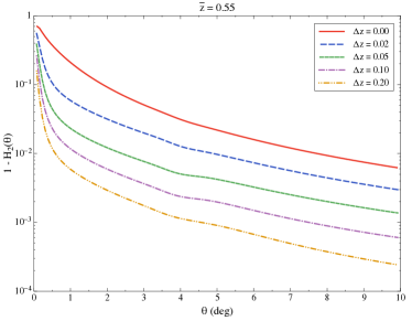
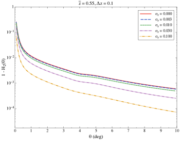
Figure 1: $\Delta H_{2}(\theta)$ as a function of $\theta$ for varying redshift bin size (left panel) and photometric redshift uncertainty (right panel). The use of thick redshift bins and photometric redshifts produces a more homogeneous distribution when projected on the sphere, reducing the amplitude of the correlation.

The three-dimensional correlation function is related to the power spectrum through a Fourier transform

$$\xi({\bf r})=\frac{1}{(2\pi)^{3}}\int\,dk^{3}\,e^{i\,{\bf k}\cdot{\bf r}}P({\bf k}).$$ (20)

The following model was used for the redshift-space power spectrum

$$P_{s}(k,\mu_{k},z)=b^{2}(z)\,(1+\beta(z)\mu_{k}^{2})^{2}\,P_{r}(k,z),$$ (21)

where $P_{r}(k,z)$ is the real-space power spectrum, $b(z)$ is the linear galaxy bias, $\beta=f/b$ is the redshift-distortion parameter and $\mu_{k}$ is the cosine of the angle between the wave vector ${\bf k}$ and the line of sight. Non-linearities were taken into account by using the HALOFIT prediction (, Smith et al.2003). The power spectra used for the theoretical predictions were provided by CAMB (, Lewis et al.2000). For the figures shown in this section we used the flat $\Lambda$CDM parameters

$$(\Omega_{M},\Omega_{\Lambda},\Omega_{b},h,\sigma_{8},n_{s})=(0.3,0.7,0.049,0.67,0.8,0.96)$$ (22)

as a fiducial cosmology.

2.4.1 Projection effects and bias

Different effects have an influence in the way the galaxy distribution approaches homogeneity. In the case that concerns us, that of data projected on the sphere, this projection effectively homogenizes the distribution. This is easy to understand: consider a pair of galaxies subtending a small angle but separated by a large radial distance. While they are far away, and therefore almost uncorrelated, they appear close when projected. This effect is obviously larger for wider redshift bins, and therefore $H_{2}(\theta)$ will approach 1 on smaller scales as we increase the binwidth. This effect is shown in the left panel of figure 1. The effect of a large photo-$z$ error is similar: the photo-$z$ shifts galaxies from adjacent redshift bins, effectively making the bin width larger (see right panel of figure 1).

On the other hand, galaxy bias modifies the homogeneity index in the opposite way. A positively biased population ($b>1$) is more strongly clustered and therefore will reach the homogeneous regime on larger scales. This can be seen in figure 2.

2.4.2 Non-linearities

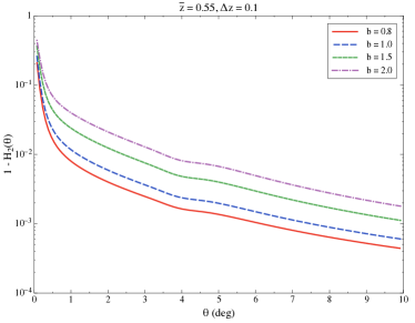
Figure 2: $\Delta H_{2}(\theta)$ as a function of $\theta$ for varying galaxy bias. A biased galaxy population will be more tightly clustered, and therefore will show a more evident departure from homogeneity.

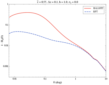
Figure 3: $\Delta H_{2}(\theta)$ as a function of $\theta$ for two different non-linearities prescriptions. Since the $H_{2}(\theta)$ depends on an integral quantity, it contains information about small scales. Thus, it is important to describe non-linear effects correctly. The solid red line corresponds to the prediction using the HALOFIT fitting formula, which fits well our mock catalogs. The prediction including only the damping of the BAO wiggles (dashed blue line) overpredicts $H_{2}(\theta)$ on small scales, although this offset decreases for larger angles.

As we said, homogeneity is reached in the standard cosmological model on relatively large scales. Therefore one might think that the modelling of the small-scale non-linear effects should be irrelevant. However, the angular homogeneity index (or the correlation dimension in 3D) depends on an integral quantity (number counts inside spheres), and therefore contains information about those small scales which may propagate to larger angles.

This is shown in figure 3, where the angular homogeneity index for the bin $z\in(0.5,0.6)$ has been plotted using different prescriptions to describe non-linearites. The solid red line shows the prediction using the HALOFIT fitting formula (which provides the best fit to the mock data in section 3). The dashed blue line corresponds to the prediction in renormalized perturbation theory (RPT) (, Crocce & Scoccimarro2006) of the damping of the BAO wiggles due to non-linear motions, given by

$$\Delta P_{\rm wiggles}^{NL}(k)=\Delta P_{\rm wiggles}^{L}(k)\,\exp(-\sigma_{v}^{2}k^{2}/2),$$ (23)

where $\Delta P_{\rm wiggles}$ is the BAO contribution to the power spectrum and

$$\sigma_{v}=\frac{1}{6\pi^{2}}\int_{0}^{\infty}P^{L}(k)\,dk.$$ (24)

As can be seen, the extra clustering amplitude on small scales contributes as a visible offset in $H_{2}$ up to scales of $\mathcal{O}(1\,{\rm deg}\sim 20\,{\rm Mpc}/h)$.

2.4.3 Dependence on cosmological parameters

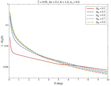
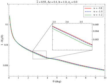
Figure 4: $\Delta H_{2}(\theta)$ as a function of $\theta$ for varying $\Omega_{m}$ (left panel) and dark energy equation of state $w$ (right panel).

Since the evolution of the matter perturbations depends on the background cosmological parameters, we can expect that some cosmological models will approach homogeneity faster than others. We have studied this dependence using our model for $H_{2}(\theta)$. Our aim is not to use the form of $H_{2}(\theta)$ to obtain precise cosmological constraints, since we do not think that this quantity contains more information than the two-point correlation function $w(\theta)$, for which there exist many different methods in the literature (, Nock et al.2010, Sanchez et al.2011, de Simoni et al.2013). However, we think that a qualitative characterization of the homogeneity index for different types of models is instructive and may give us some hints about how model-independent our results are.

In Fig. 4 we have plotted $H_{2}(\theta)$ varying the values of the matter parameter $\Omega_{M}$ (left panel) and the dark energy equation of state $w$ (right panel), from their fiducial values (eq. 22). As expected, larger values of $\Omega_{M}$ enhance the amplitude of inhomogeneities on small scales (i.e., make $\Delta H_{2}$ larger). Likewise, more negative values of $w$ accelerate the expansion and damp the growth of perturbations, shifting $H_{2}$ closer to 1. In any case we observe a mild dependence of $H_{2}$ on the cosmological parameters, and hence we expect that the results presented here should not vary qualitatively for any viable homogeneous cosmological model.

2.5 Defining homogeneity

As has been discussed, even though the stantard cosmological model postulates a homogeneous and isotropic Universe, this homogeneous regime is only approached asymptotically on large scales or in early times. Thus, there is no straightforward prescription to define the scale at which homogeneity is reached. Two different definitions have been used in the literature:

• One possibility is to define the scale of homogeneity as the scale at which the difference between our measurement of $D_{2}$ or $H_{2}$ (or, in general, any observable characterizing fractality) and its homogeneous value ($D_{2}=3$, $H_{2}=1$) is comparable with the uncertainty in this measurement. The caveat of this definition is that this uncertainty will depend on the characteristics of the survey (area, depth, number density, etc.), and therefore different surveys will measure a different scale of homogeneity. However, this is possibly the most mathematically meaningful definition.

• Another approach is to define that homogeneity is reached when the measured fractal dimension is within a given arbitrary fraction of its homogeneous value. For example, Scrimgeour et al. (2012) use a value of 1%. The advantage of this definition is that all surveys should measure the same scale of homogeneity, while its caveat is the arbitrariness of the mentioned fraction. Furthermore, using this kind of prescription would not be viable in our case, since, as we have seen, projection effects reduce the departure from homogeneity, and therefore the same fixed fraction cannot be used for different bins.

For the data analyzed in the next section, we have chosen to follow the first prescription, defining the homogeneity scale $\theta_{H}$ as the angle at which

$$\Delta H_{2}(\theta)\leq q\,\sigma_{H_{2}}(\theta),$$ (25)

where $\sigma_{H_{2}}$ is the error on $H_{2}$ and $q$ is an $\mathcal{O}(1)$ number. For this analysis we have used $q=1.96$ (i.e., assuming Gaussian errors, $\theta_{H}$ is the angle at which the measured $H(\theta)$ is away from 1 at 95% C.L.). Note that the value of $\theta_{H}$ given by this definition should be interpreted as a lower bound on the scale of homogeneity, and not as a scale beyond which all inhomogeneities disappear.

At the end of the day, the scale at which homogeneity is reached is not a well defined quantity, nor is it of vital importance. Instead, the main aim of this kind of studies is to establish whether homogeneity is reached or not, focusing on defining the limits of our ability to detect a departure from large-scale homogeneity.

3 Measuring the homogeneity index

In order to assess the performance of the different estimators for $H_{2}(\theta)$ in a realistic scenario, we have used them on a set of simulated galaxy surveys corresponding to a canonical $\Lambda$CDM model.

3.1 Lognormal mock catalogs

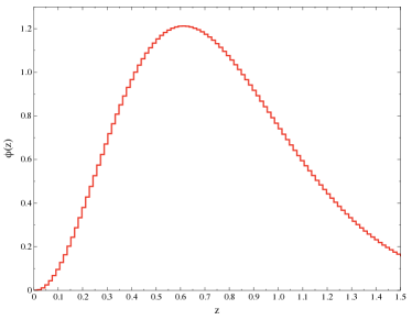
Figure 5: Selection function as a function of redshift used for the lognormal catalogs, given by eq. (26).

Lognormal fields were proposed by (, Coles & Jones1991) as a possible way to describe the distribution of matter in the Universe. More interestingly for our purposes, lognormal fields provide an easy and fast method to generate realizations of the density field in order to produce large numbers of mock catalogs. This technique has been used by different collaborations to estimate statistical uncertainties and study different systematic effects in galaxy surveys, and has been proven to be a remarkably useful tool. The physics and mathematics of lognormal realizations, as well as their limitations, have been widely covered in the literature (, Coles & Jones1991, White et al.2013), and the specific method used to generate the catalogs used in this work is described in appendix A.

100 lognormal realizations were generated for the cosmological model of equation (22) inspired by the latest measurements by the Planck collaboration (Planck Collaboration, 2013). Each catalog contains $1.2\times 10^{8}$ galaxies distributed over one octant of the sky ($\simeq 5000\,{\rm deg}^{2}$) in the redshift range $0<z<1.4$ with a selection function

$$\phi_{\rm true}(z)\propto z^{2}\,e^{-\left(\frac{z}{0.5}\right)^{1.5}},$$ (26)

shown in figure 5. The density field was generated in a box of size $L_{\rm box}=3000\,{\rm Mpc}/h$ with a grid of size $N_{\rm side}=2048$, yielding a spatial resolution of $l_{\rm grid}\simeq 1.5\,{\rm Mpc}/h$. All the catalogs contain redshift-space distortions, as described in appendix A, and a Gaussian photometric redshift error was generated for each galaxy with $\sigma_{z}=0.03\,(1+z)$. Since the effect of a linear galaxy bias factor is well understood and very easy to model in theory, all the catalogs were generated with $b=1$.

3.2 Results

3.2.1 The angular homogeneity scale $\theta_{H}(z)$

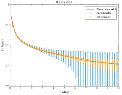
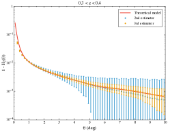
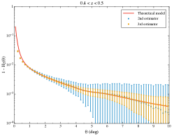
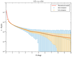
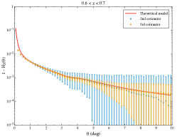
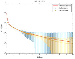
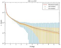
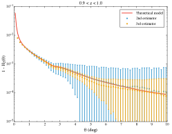
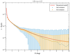
Figure 6: $\Delta H_{2}(\theta)$ as a function of $\theta$ calculated from the 100 lognormal realizations forthe 9 redshift bins given in table 1. The data contains Gaussian photometric errors with $\sigma_{z}=0.03\,(1+z)$. The blue dots with error bars correspond to the mean and standard deviation of the 100 mocks for the estimator E2, while the red dots correspond to estimator E3. The solid red line shows the theoretical model described in section 2.4.

In order to better understand the approach to homogeneity of a projected galaxy survey we have computed $H_{2}(\theta)$ from the 100 lognormal catalogs using the two estimators E2 and E3. Then, the lower limit on the angular homogeneity scale was estimated, as described in section 2.5, as the angle for which $H_{2}$ is away from 1 at 95% C.L. (i.e. $\Delta H_{2}=1.96\,\sigma_{H_{2}}$), where the errors $\sigma_{H_{2}}$ were calculated as the standard deviation of the 100 lognormal realizations (see section 3.2.2).

The comoving three-dimensional homogeneity scale is related to the angular scale $\theta_{H}$ through

$$r_{H}(z)\equiv(1+z)\,d_{A}(z)\,\theta_{H}(z),$$ (27)

where $d_{A}(z)$ is the angular diameter distance to redshift $z$.

These results are summarized in table 1, and can be visualized in figure 6. The numbers given in this table for $\theta_{H}$ correspond to the mean value obtained from the 100 lognormal mocks, and the errors correspond to the standard deviation. Two main observations must be made:

	E2		E3
Bin limits	$\theta_{H}>$	$r_{H}>$	$\theta_{H}>$	$r_{H}>$
$0.2-0.3$	$4.9$	$60$	$7.6$	$93$
$0.3-0.4$	$4.4$	$74$	$7.9$	$131$
$0.4-0.5$	$4.4$	$92$	$7.1$	$149$
$0.5-0.6$	$4.0$	$99$	$6.4$	$159$
$0.6-0.7$	$3.7$	$105$	$6.1$	$175$
$0.7-0.8$	$3.3$	$108$	$5.7$	$184$
$0.8-0.9$	$3.4$	$121$	$5.4$	$193$
$0.9-1.0$	$3.5$	$137$	$5.3$	$207$
$1.0-1.2$	$3.0$	$131$	$4.8$	$208$

Table 1: Lower bound on the scale of homogeneity calculated for the nine redshift bins of the 100 lognormal realizations. The angular scale of homogeneity $\theta_{H}$ is given in degrees, while the corresponding comoving distance is given in ${\rm Mpc}/h$.

• First, since the two estimators make a different use of the data, they have different variances, and therefore each of them measures a different lower bound on the homogeneity scale. While all the galaxies in the survey are used as centres for spherical caps of any angular aperture in the case of E3, only those caps that fit fully inside the field of view are used for E2. Thus, in this case the variance will grow faster for larger scales, and homogeneity is reached on smaller angles. This is explicitly illustrated in figure 8.

• Secondly, the comoving scale corresponding to the angular homogeneity scale for each bin seems to increase with redshift. This result is precisely the opposite of what intuition would predict: since the amplitude of matter perturbations decreases with redshift, the matter distribution is more homogeneous at earlier times, and should reach homogeneity on smaller scales at larger redshifts. This paradox is due to the fact that the definition that we have used for the scale of homogeneity is based on statistical principles, and not on the physical meaning of homogeneity. For this and other reasons we believe that producing a number for $\theta_{H}$ or $r_{H}$ is not as relevant as setting a lower limit to the departure from large-scale homogeneity that can be allowed given our observational capabilities.

3.2.2 Statistical uncertainties

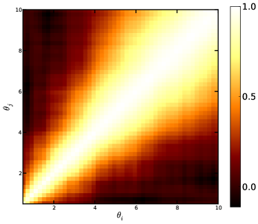
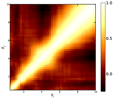
Figure 7: Correlation matrix $\rho_{i,j}\equiv C_{i,j}/\sqrt{C_{i,i}C_{j,j}}$ of $H_{2}$ for E2 (left) and E3 (right). Note that the errors are correlated over relatively wide ranges of scales, specially on large angles.

We have studied the full covariance matrix of the angular homogeneity index $H_{2}(\theta)$ for the different estimators. The covariance between the angular bins $\theta_{i}$ and $\theta_{j}$ is calculated from the measurements of $H_{2}$ in the 100 lognormal mock catalogs as

$$C_{i,j}=\frac{1}{N_{m}-1}\sum_{n=1}^{N_{m}}H_{2}^{n}(\theta_{i})H_{2}^{n}(\theta_{j})-\overline{H_{2}(\theta_{i})}\,\overline{H_{2}(\theta_{j})},$$ (28)

where $N_{m}=100$, $H_{2}^{n}$ is the measurement on the $n$-th catalog and $\overline{H_{2}}$ is the arithmetic mean over all the catalogs.

Figure 8 shows the diagonal errors $\sigma_{i}\equiv\sqrt{C_{i,i}}$ for the bin $z\in(0.5,0.6)$ using the estimators E2 and E3. As was noted before, the errors corresponding to E2 are significantly larger than those of E3 for large scales, due to the smaller number of galaxies used as centres of spherical caps for those angles.

The correlation matrix $\rho_{i,j}\equiv C_{i,j}/\sqrt{C_{i,i}C_{j,j}}$ is shown, for the same two estimators and the same bin, in figure 7. As is shown in the figure, the measurements of $H_{2}$ are statistically correlated over wider ranges of scales as we go to larger angles, especially in the case of E2. Therefore, if any likelihood analysis is to be done on $H_{2}$, the full covariance matrix must be used.

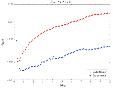
Figure 8: Diagonal errors on $H_{2}(\theta)$ as a function of $\theta$ for estimators E2 (red) and E3 (blue). Since with E3 all galaxies are used as centres of spherical caps for all $\theta$, the errors are significantly smaller than in the case of E2.

3.2.3 Projection effects

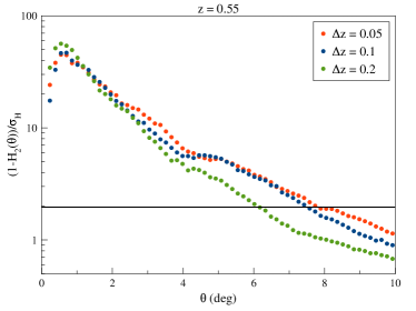
Figure 9: Departure from homogeneity $\Delta H_{2}$ divided by the uncertainty on $\sigma_{H_{2}}$ as a function of $\theta$ for a redshift bin centered on $\bar{z}=0.55$ with different binwidths. As could be expected, projecting on wider bins moves the scale of homogeneity towards smaller angles.

As has been said before, using wider redshift bins damps the amplitude of the correlation function and makes the projected galaxy distribution more homogeneous (i.e., $H_{2}$ gets closer to 1). However, the amplitude of the error on the correlation function (or on $H_{2}$) will also be damped, and it is therefore interesting to study whether the two dampings compensate each other and to quantify the effect on the scale of homogeneity. This has been done in figure 9. The homogeneity index $H_{2}(\theta)$ has been calculated at $\bar{z}=0.55$ using different redshift binwidths: $\Delta z=0.05,\,0.1,\,0.2$, and the ratio $\Delta H_{2}/\sigma_{H_{2}}$ has been plotted for different values of $\theta$. According to our definition, the homogeneity scale is reached when this ratio becomes 1.96. As can be seen, the damping of $\Delta H_{2}$ due to projection effects is not compensated by the corresponding damping on $\sigma_{H_{2}}$, and the homogeneous regime is reached on smaller scales for wider bins, as could be intuitively expected. Since the use of photometric redshifts effectively increases the width of the redshift bin, it produces a similar effect.

3.2.4 Fraction of the sky

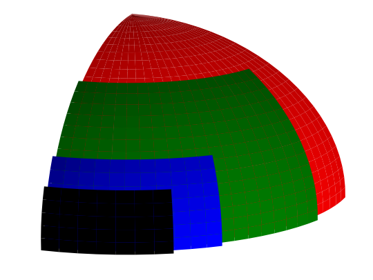
Figure 10: The four survey cases considered in section 3.2.4, covering $5000\,{\rm deg}^{2}$ (red), $3000\,{\rm deg}^{2}$ (green), $1000\,{\rm deg}^{2}$ (blue) and $500\,{\rm deg}^{2}$ (black).

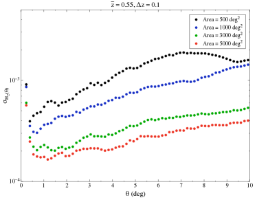
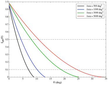
Figure 11: Left panel: Errors on $H_{2}(\theta)$ for the four surveys described in figure 10 as a function of $\theta$. Right panel: Fraction of complete spheres of different radii in the same four surveys as a function of $\theta$. The horizontal dashed lines correspond to the last two criteria considered below to determine the maximum angular scale to be used.

	Crit. 1		Crit. 2		Crit. 3
Area	$\theta_{\rm max}$	$\Delta H_{2}^{\rm min}\times 10^{3}$	$\theta_{\rm max}$	$\Delta H_{2}^{\rm min}\times 10^{3}$	$\theta_{\rm max}$	$\Delta H_{2}^{\rm min}\times 10^{3}$
$5000\,{\rm deg}^{2}$	$35^{o}$	$0.08\pm 1$	$25^{o}$	$0.08\pm 0.8$	$10^{o}$	$0.2\pm 0.35$
$3000\,{\rm deg}^{2}$	$25^{o}$	$0.08\pm 1.5$	$19^{o}$	$0.09\pm 0.9$	$8^{o}$	$0.4\pm 0.5$
$1000\,{\rm deg}^{2}$	$13^{o}$	$0.12\pm 1.7$	$10^{o}$	$0.2\pm 1.4$	$4.5^{o}$	$1.0\pm 0.7$
$500\,{\rm deg}^{2}$	$9^{o}$	$0.3\pm 2$	$7^{o}$	$0.33\pm 1.7$	$3^{o}$	$1.8\pm 0.8$

Table 2: Constraints on the level of homogeneity $\Delta H_{2}^{\rm min}\equiv 1-H_{2}(\theta_{\rm max})$ attainable with surveys of different areas for the three criteria described in section 3.2.4 for the maximum angular scale $\theta_{\rm max}$.

In order to study the effects related to the area covered by a given survey, we considered a fiducial redshift bin $0.5<z<0.6$ and restricted the data from our mock catalogs to regions of different areas. Specifically, we have considered surveys covering $\sim 5000\,{\rm deg}^{2}$ (one octant of the sky) $\sim 3000\,{\rm deg}^{2}$, $\sim 1000\,{\rm deg}^{2}$ and $\sim 500\,{\rm deg}^{2}$. For simplicity we have used simply connected fields of view with the shapes shown in figure 10. This is an ideal scenario, and therefore the results shown here would correspond to the most optimistic ones any survey of the same area could obtain. The total area covered by a given survey affects the measurement of $H_{2}(\theta)$ in two ways.

First, the sample variance should be inversely proportional to $\sqrt{f_{\rm sky}}$ (, Crocce et al.2010), and therefore the uncertainty in $H_{2}$ will grow for smaller areas. This is illustrated in the left panel of figure 11, which shows the magnitude of the errors on $H_{2}$ for the 4 different areas.

Secondly, the survey size limits the maximum scale that we are able to probe, and may prevent us from reaching the homogeneous regime. In order to illustrate this point, we have performed the following exercise: inside each of the regions shown in figure 10, we have randomly placed a large number points. Then, for different values of $\theta$, we have estimated the fraction of spherical caps of radius $\theta$ centered on these points that lie fully inside the surveyed region. The result is shown in the right panel of figure 11. In view of this result we have established three different criteria to define the largest scale $\theta_{\rm max}$ that can be probed in a survey:

1. $\theta_{\rm max}$ corresponds to the radius of the largest spherical cap that fits inside the surveyed region.

2. $\theta_{\rm max}$ is the angle for which the fraction shown in the right panel of figure 11 is 10%.

3. The same as above for a fraction of 50%.

For each of these criteria and for the 4 different areas we have listed in table 2 the minimum value of $\Delta H_{2}$ that can be obtained together with its uncertainty $\sigma_{H_{2}}$.

4 Robustness of the method

Since the use of random catalogs to correct for mask and edge effects may bias the estimation of $H_{2}(\theta)$ towards homogeneity, it is important to study the relevance of this effect. Furthermore, it has been argued (, Durrer et al.1997) that fractal distributions may look homogeneous when projected onto the celestial sphere, and therefore it is necessary to verify that we are indeed able to distinguish a 3D fractal from an asymptotically homogeneous distribution using only angular information, and to what level so. In order to address these questions, we have analyzed different inhomogeneous models which, we know, should not approach homogeneity.

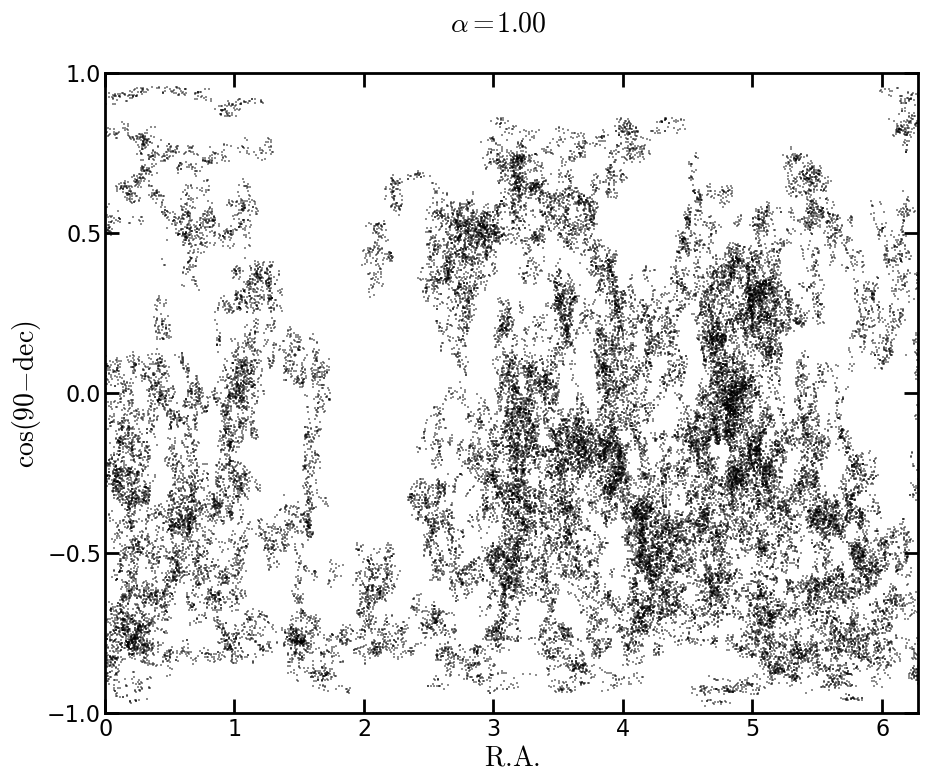
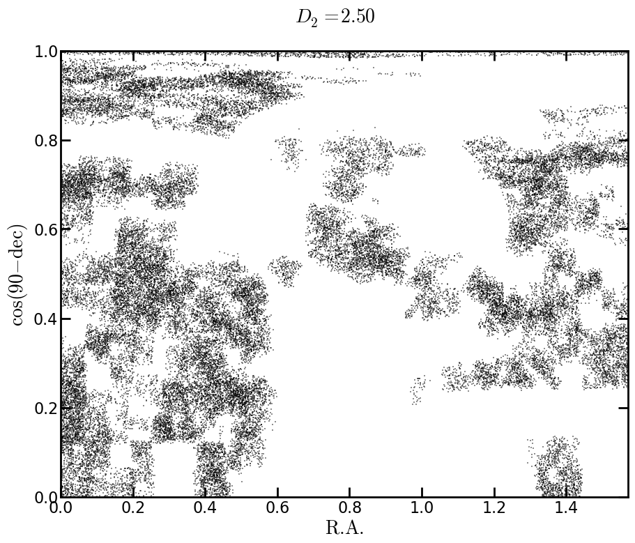
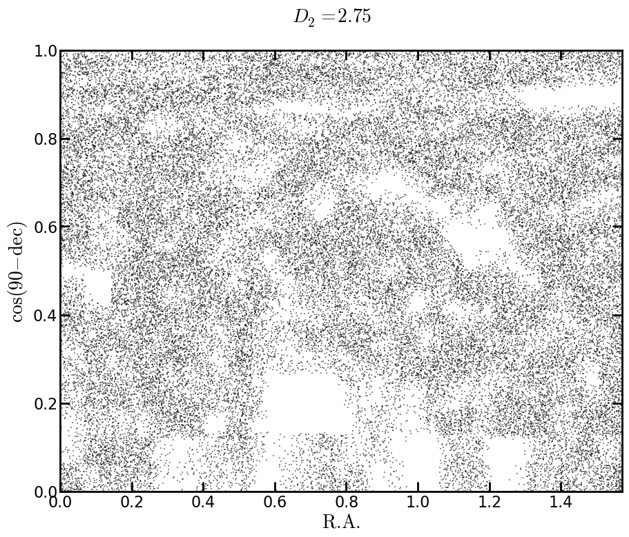
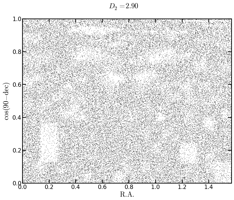
Figure 12: Sky maps for the 2D Rayleigh-Levy flights (left) and the $\beta$-model catalogs at $0.5<z<0.6$ (right). The plots are ordered top-down from more to less inhomogeneous.

4.1 Spherical Rayleigh-Levy flights

A random walk in 3 dimensions is an iterative point process in which the distance between one point and the next one is drawn from a probability distribution independently of all previous jumps. In the particular case of a heavy-tailed Pareto distribution

$$P(r>R)=\left\{\begin{array}[]{lr}1&R<R_{0}\\ \left(\frac{R}{R_{0}}\right)^{-\alpha}&R\geq R_{0}\end{array}\right.,$$ (29)

these walks are called Lévy flights and exhibit a fractal behavior with $D=\alpha$ for $\alpha\leq 2$ (, Nusser & Lahav2000).

We have generated random walks on the sphere by following a similar process. We first choose a starting point on the sphere at random, and draw an angular distance $\theta_{d}$ from a probability distribution. The next point is selected at this distance in an arbitrary direction from the first one, and the process is repeated. For our walks we have chosen a distribution similar to the one given above in the three-dimensional case

$$P(\theta_{d}<\theta)=\left\{\begin{array}[]{lr}1&\theta<\theta_{0}\\ \left(\frac{1-\cos\theta}{1-\cos\theta_{0}}\right)^{-\alpha}&\theta\geq\theta_{0}\end{array}\right..$$ (30)

It must be noted that with this procedure we are generating an inhomogeneous distribution directly in the 2-dimensional sphere, and not projecting a 3-dimensional set. However we know for sure that this distribution must asymptotically reach some $H_{2}(\theta)\neq 1$, and therefore we can use it to verify that the use of random catalogs does not bias our results. To do so we have considered values of $\alpha=0.5,\,0.75\,\text{and}\,1$, generating 20 random walks containing $10^{6}$ objects in all cases. Figure 12 (left column) shows the 2D distribution of some of these walks for different values of $\alpha$, showing that the degree of ihomogeneity increases with $\alpha$.

We have calculated $H_{2}(\theta)$ and its error from these random walks using the E3 estimator. The results are shown in figure 13 together with those corresponding to the $\Lambda$CDM lognormal catalogs. In all cases the asymptotic value of $H_{2}$ is different from 1 and can be clearly distinguished from the $\Lambda$CDM prediction, showing that, at least within the range of scales explored, our method is not biased towards homogeneity.

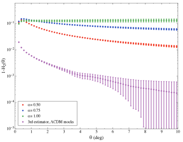
Figure 13: $\Delta H_{2}(\theta)$ as a function of $\theta$ for three sets of 2D Rayleigh-Levy flights with $\alpha=1.0$ (green), $\alpha=0.75$ (blue) and $\alpha=0.5$ (red), together with the result from the lognormal catalogs for the bin $0.5<z<0.6$ (purple).

4.2 $\beta$-model

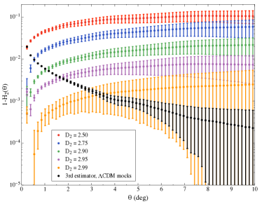
Figure 14: $\Delta H_{2}(\theta)$ as a function of $\theta$ for the $\beta$-models projected onto the redshift bin $0.5<z<0.6$ for different values of $D_{2}$ from 2.5 (top) to 2.99 (bottom), together with the $\Lambda$CDM prediction obtained from the lognormal mocks (black). In spite of the 2D projection, we are still able to distinguish the inhomogeneous nature of the $\beta$-model from an asymptotically homogeneous model for $D\lesssim 2.95$.

The fractal $\beta$-model (see (Castagnoli & Provenzale1991)) is a multiplicative cascading fractal model based on the following process: take a cubic box of side $L$ and perform $N_{\rm side}$ equal divisions per side. Then, give a probability $p<1$ to each of the $N_{\rm side}^{3}$ sub-cubes of surviving to the next iteration and randomly choose those which survive according to this probability. In the next iteration you follow the same process on each of the surviving sub-cubes. In the $n$-th iteration, the average number of surviving cells will be $N_{\rm surv}=(N_{\rm side}^{3}\,p)^{n}$. Equating this to $N_{\rm side}^{n\,D}$ we obtain that this set has a fractal dimension

$$D=3+\log_{N_{\rm side}}p.$$ (31)

We explored different values for $D$ ranging from 2.5 to 3, generating multiple realizations of this process for each value. These catalogs were produced by running the process outlined above on a cubic box of the same size as the one used for the lognormal catalogs, using $N_{\rm side}=2$. The catalog is then subsampled to the desired number density and the three-dimensional distances to each object are translated into redshifts using our fiducial cosmological parameters. This is, of course, not correct, since the distance-redshift relation for this model need not be that of FRW, however it is not clear which relation should be used. In any case, our aim is to explore whether a three-dimensional inhomogeneous model could be noticed when projected onto the sphere, and, for this purpose, our choice of $\chi(z)$ is as good as any other. The redshift of each object is then perturbed with a Gaussian photo-$z$ error with $\sigma_{z}=0.03\,(1+z)$, and the point distribution is projected in different redshift bins.

The projected distributions of some of these catalogs for a redshift bin $0.5<z<0.6$ are shown in figure 12 (right panel). Figure 14 shows the value of $H_{2}(\theta)$ and its error calculated from these catalogs for a the same bin, together with the $\Lambda$CDM result from the lognormal catalogs. As is evident from this figure, when projected, these catalogs still retain their inhomogeneous nature, and can be clearly distinguished from an asymptotically homogeneous $\Lambda$CDM model for values of $D_{2}$ that are remarkably close to 3. For instance, only with the results drawn from the bin $0.5<z<0.6$ we would be able to set the limit $D_{2}\gtrsim 2.95$.

4.3 LTB models

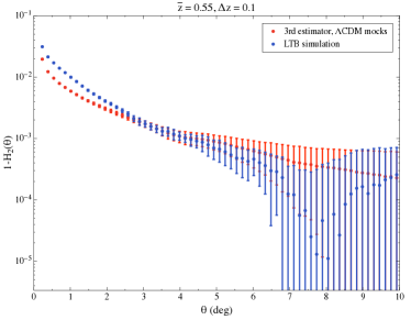
Figure 15: $\Delta H_{2}(\theta)$ as a function of $\theta$ for an LTB void model (blue) compared to the $\Lambda$CDM value (red). Since the LTB metric preserves spherical homogeneity around the central observer, the inhomogeneity of these models can not be measured using the method described in this paper.

In general there is no direct connection between the three dimensional fractal dimension $D_{2}$ and the homogeneity index $H_{2}$ of the projected data. An extreme example of this would be an inhomogeneous but spherically symmetric distribution in which the observer sits exactly at the centre of symmetry. Although the distribution is inhomogeneous in three dimensions ($D_{2}\neq 3$), the central observer will measure a homogeneous distribution for the projected data ($H_{2}=1$).

This is precisely the case of Lemaître-Tolman-Bondi (LTB) void models. A complete description of these models is out of the scope of this paper and the reader is referred to (Clarkson et al.2012) for further information. For our purposes it is sufficient to know that, in an LTB model the observer is placed very close to the centre of a very large ($\mathcal{O}(1)\,{\rm Gpc}$) spherical underdensity. With this setup it is possible to reproduce many of the observational effects that can be adscribed to a Dark Energy component without introducing any exotic species or new physics in the model. The price to pay for this is relatively high, since in order to match the observed high isotropy of the distribution of CMB anisotropies, the observer is bound to be within a comparatively small distance ($\mathcal{O}(10)\,{\rm Mpc}$) from the centre of the void. LTB models have been tested against multiple cosmological observations (, Garcia-Bellido & Haugboelle2008, Bull et al.2012, Zumalacarregui et al.2012) and are basically ruled out. However, they provide an explicit example of an inhomogeneous model that can not be distinguished from a homogeneous distribution with our method. This is shown in figure 15, in which we compare the homogeneity index $H_{2}(\theta)$ measured from the $\Lambda$CDM mock catalogs with the values measured from an N-body simulation of an LTB model. These simulations are described in (Alonso et al.2010), and the data shown in figure 15 correspond to the best resolved simulation, labelled $\mathcal{H}$ in the aforementioned paper. The errors shown for the LTB data points have been calculated by splitting the simulation into 8 octants of the sky and then calculating the standard deviation of the 8 subsamples.

5 Summary & Discussion

In this paper we have studied the possibility of measuring the transition to homogeneity using photometric redshift catalogs. The method presented here is an extension of the usual fractal studies that have previously been performed using three-dimensional distances by several collaborations. Photometric redshift uncertainties erase much of the clustering information along the radial direction. Thus, our method is based on measuring the fractality of the projected galaxy distribution, using only angular distances. This method is assumption-free, since it relies only on observable quantites (as opposed to three-dimensional distances, which require a fiducial cosmological model), and in this sense provides a way to test the Cosmological Principle in a model-independent way. In the era of precision cosmology, testing this fundamental assumption is extremely important, and the upcoming galaxy surveys, covering large volumes of the Universe, will make this possible.

We have tested that our method is not biased by the use of random catalogs to correct for artificial effects induced on the observed galaxy distribution. We have done so by using our method on different synthetic inhomogeneous catalogs. We have verified that, not only is our method unbiased in practice, but it is in fact capable of discriminating some fractal models with relatively large fractal dimensions, in spite of the loss of information due to the radial projection. Our method is unable to detect the large-scale inhomogeneity along the line of sight, and therefore can not be used to constraint a particular type of “malicious” inhomogeneous models preserving the isotropy around a central observer.

We have modelled and studied how different effects would affect the measurement of the angular homogeneity index $H_{2}(\theta)$ in a $\Lambda$CDM cosmology. We have studied the influence of the redshift bin width, photometric redshift errors, bias, non-linear clustering, and surveyed area. The level to which a given survey will be able to constrain the transition to homogeneity will depend mainly on two factors:

• The total surveyed area: this regulates the size of the statistical uncertainties.

• The compactness of the surveyed region: this determines the largest angular scale that can be measured.

In particular, a DES-like survey should be able to easily discriminate certain fractal models with fractal dimensions as large as $D_{2}=2.95$. We believe that this method will have relevant applications for upcoming large photometric redshift surveys, such as DES or LSST.

Appendix A Lognormal mock galaxy catalogs

For the analysis described in this paper we generated 100 lognormal realizations using the following method:

1. Consider a cubic box of side $L$ and divide it into $N_{\rm side}^{3}$ cubical cells of size $l_{c}\equiv L/N_{\rm side}$. This will determine the scales available in the catalog: $2\pi/L\lesssim k\lesssim 2\pi/l_{c}$.

2. We generate a realization of the Fourier-space Gaussian overdensity field at $z=0$ by producing Gaussian random numbers with variance

   $$\sigma^{2}(k)\equiv\left(\frac{L}{2\pi}\right)^{3}P(k).$$ (32)

   This is done in a Fourier-space grid for ${\bf k}={\bf n}\,2\pi/L$ with $-N_{\rm side}/2\leq n_{i}\leq N_{\rm side}/2$.

   At the same time, the $z=0$ velocity potential can be calculated from the overdensity field as

   $$\varphi_{\bf k}(z=0)=f_{0}\,H_{0}\,\frac{\delta_{\bf k}(z=0)}{k^{2}}$$ (33)

3. Transform these fields to configuration space using a Fast Fourier Transform, and calculate the radial velocity at each cell by projecting the gradient of the velocity potential along the line of sight (LOS) (the direction of the LOS will depend on the position of the observer inside the box). This will yield the Gaussian overdensity $\delta_{G}$ and radial velocity $v_{r}$ fields at $z=0$. Note that, at this stage, we are assuming that the velocity field is purely irrotational, and that all vector contributions have died away.

4. Calculate the overdensity field and radial velocity in the lightcone by computing the redshift to each cell through the distance-redshift relation

   $$\chi(z)=\int_{0}^{z}\frac{dz^{\prime}}{H(z^{\prime})},$$ (34)

   and evolving the fields self-similarly to that redshift.

   At the same time we may perform the lognormal transformation on the Gaussian overdensity field. Thus, in a cell at ${\bf x}$ with redshift $z({\bf x})$, the overdensity and radial velocity are given by

   $$1+\delta({\bf x})=\exp\left[G(z)\delta_{G}({\bf x},z=0)-G^{2}(z)\,\sigma_{G}^{2}/2\right],$$ (35)

   $$v_{r}({\bf x})=\frac{f(z)H(z)D(z)}{(1+z)\,f_{0}\,H_{0}}\,v_{r}({\bf x},z=0),$$ (36)

   where $\sigma_{G}^{2}\equiv\langle\delta_{G}^{2}\rangle$ is the variance of the Gaussian overdensity at $z=0$ and the factor $G(z)\equiv D(z)\,b(z)$ accounts both for the growth of perturbations and a possible linear galaxy bias $b$.

5. Calculate the mean number density of objects in each cell as $n({\bf x})\equiv\bar{n}(z)\,(1+\delta({\bf x}))$, where $\bar{n}(z)$ is the desired redshift distribution. The number of galaxies in each cell is calculated by generating a Poisson random number with mean $n({\bf x})$. These galaxies are placed at random within each cell (thus losing any information about the clustering on scales below the cell resolution). The redshift of each galaxy is calculated using the distance-redshift relation and RSDs are produced by perturbing this redshift with $\Delta z_{\rm RSD}=(1+z)\,v_{r}({\bf x})$.

References

- (1) Abbott T. et al. [Dark Energy Survey Collaboration], astro-ph/0510346.
- (2) Alonso D., Garcia-Bellido J., Haugbolle T. and Vicente J., Phys. Rev. D 82 (2010) 123530
- Amendola & Palladino (1999) Amendola, L., & Palladino, E. 1999, ApJ Vol. 514 pp L1-L4
- (4) Asorey J., Crocce M., Gaztanaga E., Lewis A., 2012, arXiv:1207.6487 [astro-ph.CO]
- Bagla et al. (2007) J. S. Bagla, J. Yadav and T. R. Seshadri, 2007, MNRAS, 390:829
- Bonvin & Durrer (2011) Bonvin C. and Durrer R., 2011, PRD, 84:063505
- (7) Bull P., Clifton T. and Ferreira P. G., Phys. Rev. D 85 (2012) 024002
- (8) Castagnoli C. and Provenzale A. 1991, A&A, 246,634
- (9) Clarkson C., Comptes Rendus Physique 13 (2012) 682
- Coleman & Pietronero (1992) Coleman, P. H., & Pietronero, L. 1992, Phys. Rep., 213, 311C
- (11) Coles P. & Jones B. 1991, MNRAS, 248, 1
- (12) Crocce M. & Scoccimarro R. 2006, PRD, 73, 063519
- (13) Crocce M., Cabre A. and Gaztanaga E., 2011, MNRAS, 414:329
- (14) de Simoni F., et al. 2013, arXiv:1308.0630 [astro-ph.CO]
- (15) Durrer, R., Eckmann, J.-P., Sylos Labini, F., Montuori, M., & Pietronero, L. 1997, EPL (Europhysics Letters), 40, 491
- Durrer (2011) Durrer R. 2011, Phil. Trans. Roy. Soc. Lond. A, 369:5102
- (17) Garcia-Bellido J. and Haugboelle T., JCAP 0804 (2008) 003
- Guzzo (1997) Guzzo, L. 1997, NewA, 2, 517
- Hogg et al. (2005) Hogg D. W., et al., 2005, ApJ, 624:54
- Joyce et al. (1999) Joyce, M., Montuori, M., & Sylos Labini, F. 1999, ApJL, 514, L5
- Kurokawa et al. (2001) Kurokawa, T., Morikawa, M., & Mouri, H. 2001, A&A, 370, 358
- (22) Lewis, A., Challinor, A., & Lasenby, A. 2000, ApJ, 538, 473
- Martínez & Coles (1994) Martinez, V. J., & Coles, P. 1994, ApJ, 437, 550
- Martinez et al. (1998) Martinez, V. J., 1998, MNRAS, 298, 1212
- (25) Martinez V. & Saar E., 2002, Statistics of the galaxy distribution. CRC Press.
- Montuori et al. (1997) Montuori, M., et al., 1997, EPL (Europhysics Letters), 39, 103
- Nadathur (2013) Nadathur, S. 2013, MNRAS, 434, 398
- (28) Nock K., Percival W. J. & Ross A. J. 2010, MNRAS, 407, 520
- (29) Nusser A. & Lahav O. 2000, MNRAS, 313, L39
- Pan & Coles (2000) Pan, J., & Coles, P. 2000, MNRAS, 318, L51
- Pietronero et al. (1997) Pietronero, et al., 1997, Critical Dialogues in Cosmology, 24
- Planck Collaboration (2013) Planck Collaboration, 2013, astro-ph.CO:1303.5076
- (33) Sanchez E., et al. 2011, MNRAS, 411, 277
- Sarkar et al. (2009) Sarkar, P., et al., 2009, MNRAS, 399, L128
- Scaramella et al. (1998) Scaramella, R., et al. 1998, A&A, 334, 404
- Scrimgeour et al. (2012) Scrimgeour, M., et al., 2012, MNRAS, 425, 116
- (37) Smith, R. E., Peacock, J. A., Jenkins, A., et al. 2003, MNRAS, 341, 1311
- Sylos Labini & Amendola (1997) Sylos Labibi, F., & Amendola, L. 1997, ApL&C Vol. 36 pp 59-63
- Sylos Labini et al. (1998) Sylos Labini, F., et al., 1998, Phys. Rep., 293, 61
- Sylos Labini et al. (2009) Sylos Labini, F., Vasilyev, N. L., & Baryshev, Y. V., 2009, A&A, 508, 17
- Sylos Labini (2011) Sylos Labini, F., 2011, EPL (Europhysics Letters), 96, 59001
- (42) White M., Tinker J. L. & KMcBride C., arXiv:1309.5532 [astro-ph.CO].
- Yadav et al. (2005) Yadav, J., et al., 2005, MNRAS, 364, 601
- Yadav et al. (2010) Yadav J. K., Bagla J. S. and Khandai N., 2010, MNRAS, 405:2009
- (45) Zumalacarregui M., Garcia-Bellido J. and Ruiz-Lapuente P., JCAP 1210 (2012) 009