The Petri-Nets to Statecharts Transformation Case

This paper describes a case study for the sixth Transformation Tool Contest. The case is based on a mapping from Petri-Nets to statecharts (i.e., from flat process models to hierarchical ones). The case description separates a simple mapping phase from a phase that involves the step by step destruction Petri-Net elements and the corresponding construction of a hierarchy of statechart elements. Although the focus of this case study is on the comparison of the runtime performance of solutions, we also include correctness tests as well as bonus criteria for evaluating transformation language and tool features.

1 Introduction

Although transformations are already developed for decades in various communities (such as the compiler community [3], the program transformation community [7] and the business process management (BPM) community [10]), it is relatively new to study the strengths and weaknesses of transformation approaches across community boundaries. The aim of the Transformation Tool Contest (TTC) is to compare the expressiveness, the usability and the performance of graph and model transformation tools along a number of selected case studies. A deeper understanding of the relative merits of different tool features will help to further improve graph and model transformation tools and to indicate open problems [8]. This paper proposes a case for the sixth edition of TTC (i.e., to TTC’13).

1.1 Context of the Case

In BPM research and practice, transformations are usually programmed using general purpose programming languages. Mapping rules in BPM literature tend to be formalized using mathematical set constructs whereas they tend to be documented using informal visual rules and implemented in Java or another general purpose programming language. In the graph and model transformation communities, special purpose languages and tools are being developed to support the direct execution of such mapping rules. Finally, various comparative studies have been contributed to the emerging field of transformation engineering (cfr., [14, 18, 11, 9, 13, 12, 2, 15]) but too little transformation problems have been considered that are considered challenging by the BPM community. This paper proposes the so-called PN2SC case, related to the transformation of Petri-Nets to statecharts. The case relates to an active research line at Eindhoven University of Technology. Interestingly, much of the associated research efforts have been spent on an optimization algorithm which turns out to be irrelevant when using a rule-based transformation approach instead of an imperative programming approach [17]. Therefore, the case can be considered a nice showcase for demonstrating to the BPM community the potential impact of results from the transformation community.

1.2 Relevance for TTC’13

Besides providing input to BPM industry and its research community, this study also covers a previously unstudied type of transformation. More specifically, the transformation problem under study is a process model translation that raises the abstraction level. Regardless of concrete language and metamodel details, this type of problem has not yet been considered for the evaluation of transformation approaches.

In the following, we briefly survey existing comparative studies related to process models. Varró et al. studied various approaches to mapping conceptual process model in UML to more technical CSP models  [18]. Also, in a special issue edited by Rensink et al., various experts present their solutions to a case study concerning the mapping of conceptual process models in BPMN to more technical BPEL models [11]. Grønmo et al. discuss various approaches to transforming conceptual UML models into strictly structured counter-parts [9]. Again, the target models are more low-level than the input models. Rose et al. discuss different approaches to migrating Petri-Net models [12]. In that case, input models are at the same level of abstraction as output models.

Van Gorp et al. have already considered the case proposed by this paper for comparing a graph transformation approach to the Java-based programming approach that is mainstream in the BPM domain. The authors make the interesting observation that the rule-based approach required less specification effort yet delivered superior performance. By submitting this case to TTC’13, we aim at analyzing the generalizability of that observation.

2 The Transformation

This section details the Petri-Net to statechart transformation algorithm, originally described by Eshuis [4]. We summarise the key details of the transformation below, and strongly encourage solution developers to refer to [4] for a more comprehensive discussion of the transformation and the rationale behind the transformation rules. The transformation described below is input-destructive (elements of the Petri-Net model are removed as the transformation proceeds), and uses the metamodels shown in figure 1. Variants of the rules can be designed such that the input model is not destroyed. However, in order to make all solutions comparable at the level of languages and tools, discourage unnecessary variations at the solution design level. In general, we encourage solution submitters to stick as closely as possible to the conceptual requirements, as described in the following.

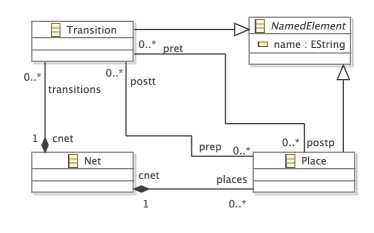
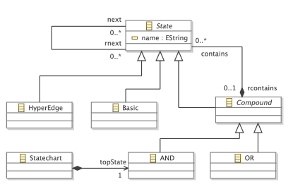
(a) Petri-Net metamodel (b) Statechart metamodel

Figure 1: The metamodels used in the PN2SC transformation.

2.1 Preconditions

The following assumptions can be made regarding the context in which the PN2SC transformation is started:

• there is only one instance of Net,

• there are no Statechart nor State instances.

2.2 Initialization

The first step in the PN2SC transformation involves creating an initial structure for the statechart model. In particular, the following statechart model elements are created:

• For every Place $p$ in the Petri-Net:

  an instance of Basic, $b$ (with $b.name=p.name$),

  an instance of OR, $o$ such that $o.contains=\{b\}$,

• For every Transition $t$ in the Petri-Net:

  an instance of HyperEdge $e$ (with $e.name=t.name$),

• All pret/postp and postt/prep arcs should be mapped to next/rnext links between the States equivalent with the input NamedElements that are connected by these arcs.

Equivalence.

Initialization should also provide a mechanism for identifying the OR node created for a particular Place and the HyperEdge created for a particular Transition. The precise mechanism can vary over implementations. One approach is to use a name-based identification (e.g., assign all Places a uniquely identifying name and copy each Place’s name to its OR node during initialization.) Another approach is to create traceability links between corresponding source and target elements. In the remainder of this section we assume that the initialization of the transformation will construct an injective function $equiv:Place\to OR$.

2.3 Reduction rules

Following initialization, the transformation continues by applying one of two types of reduction rules: AND and OR.

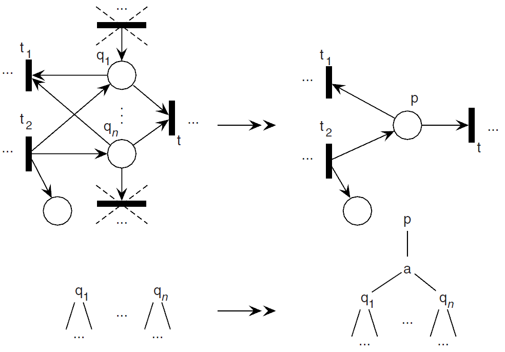
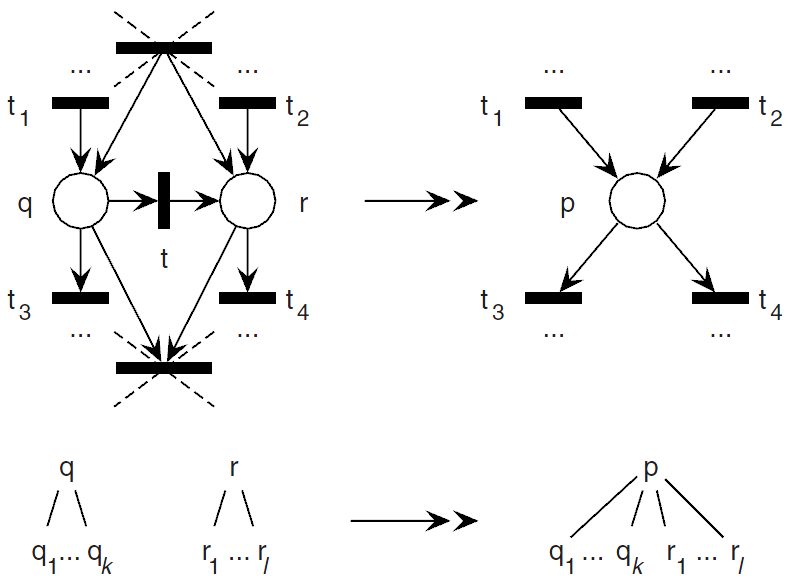
(a) rule for creating AND nodes (b) rule for merging OR nodes

Figure 2: Visual documentation for mapping rules.

2.3.1 AND rules

The first type of reduction rule, AND (informally documented by Figure 2.a), constructs an AND state for a set of Places that are connected to the same incoming and outgoing Transitions.

Pre-conditions.

The AND rule can be applied to a Transition, $t$, iff $\left|t.prep\right|>1$ and every Place in $t.prep$ is connected to the same set of outgoing transitions and the same set of incoming transitions. Alternatively, the AND rule can be applied to a Transition, $t$ iff $\left|t.postp\right|>1$ and every Place in $t.postp$ is connected to the same set of outgoing transitions and the same set of incoming transitions. Given these two alternative situations, we refer to two AND rules. However, in some languages one can implement these variants in one rule.

Figure 2.a illustrates when the AND rule for the situation $\left|t.prep\right|>1$ would be applicable: $q_{1}$ to $q_{n}$ all have $\{t,t_{1},...\}$ as the set of outgoing transition, and they share $\{t_{2},...\}$ as the set of incoming transitions. $q_{n}$ should not have an outgoing arc to a transition for which there is no corresponding arc between $q_{1}$ and that transition. Conversely, $q_{1}$ should not have an incoming arc from a transition for which there is no corresponding arc between that transition and $q_{n}$. To illustrate the situation when the AND rule for the situation $\left|t.postp\right|>1$ would be applicable, one can simply reverse all arcs in Figure 2.a.

Effect on statechart.

Applying the AND rule results in the creation of a new AND state ($a$) and a new OR state ($p$) such that $p.contains={a}$ and $a.contains$ is the set of OR states $\{q\in t.prep:equiv(q)\}$; or $\{q\in t.postp:equiv(q)\}$ if the rule has been applied to the transition’s postset, $t.postp$.

Effect on Petri-Net.

Applying the AND rule removes from the Petri-Net all but one of the Places in the set $t.prep$ ($t.postp$).

Example Implementations.

An EOL implementation of the AND rule can be found online. That EOL solution applies to the cases $\left|t.prep\right|>1$ and $\left|t.postp\right|>1$ without requiring code duplication. A GrGen.NET implementation based on two separate variants of the AND rule can also be found online.

2.3.2 OR rules

The second type of reduction rule, OR (informally documented by Figure 2.b), constructs an OR state for a Transition that has a single preceding Place and single succeeding Place.

Pre-conditions.

The OR rule can be applied to a Transition, $t$, iff $(\left|t.prep\right|=1)\land(\left|t.postp\right|=1)$ and there is no transition, $t^{\prime}$, such that $(q\in t^{\prime}.prep)\land(r\in t^{\prime}.prep)$ or $(q\in t^{\prime}.postp)\land(r\in t^{\prime}.postp)$ where $q$ is the single place contained in $t.prep$ and $r$ is the single place contained in $t.postp$.

Effect on statechart.

Applying the OR rule results in the creation of a new OR state ($p$) such that $p.contains$ is the set of OR states $equiv(q).contains\cup equiv(r).contains$.

Effect on Petri-Net.

Applying the OR rule removes from the Petri-Net the Transition $t$ and the Places $q$ and $r$; and adds a new Place $p$ such that $p.pret=(q.pret\cup r.pret)$ and $p.postt=(q.postt\cup r.postt)$.

Example Implementations.

An EOL implementation of the OR rule can be found online. This implementation re-uses $q$ to form $p$, rather than instantiate a new Place or OR state). A GrGen.NET implementation can also be found online.

2.4 Termination

The output model should contain a single instance of Statechart $sc$. The transformation should apply the reduction rules as long as possible to the input elements. For input Petri-Nets in the class of nets defined by [5], the reduction process should terminate with exactly one Place left. The equivalent AND state $st$ should not have any parent Compound state. Moverover, $sc.topState=st$ should hold for $sc$. For input nets outside that class, the reduction rules typically cannot produce a unique top-level AND state so it is impossible to produce a model that conforms strictly to the output model. However, in that case the transformation should terminate in a state that can only be reached after sequentially applying the reduction rules as long as possible. It should be possible to inspect the resulting state of the input Petri-Net for further analysis purposes.

3 Example Transformation Execution Trace

This section demonstrates the intended behavior of the reduction rules from the previous section. Figure 3 visualizes an execution trace for an input model with 11 places and 10 transitions. The input Petri-Net model is shown on the left of the figure while its corresponding statechart is shown at the right of the figure. Places are represented as white circles and transitions as black bars. Basic states are represented as yellow ovals while hyperedges are represented as black bars too. OR states are represented as white boxes while AND states are represented as gray boxes. The top of the figure shows an execution snapshot after initialization. Each Place and Transition element has respectively its corresponding Basic state and HyperEdge.

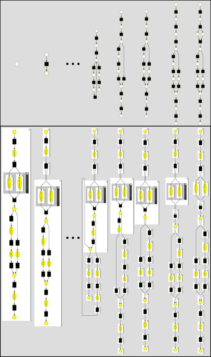
Figure 3: Visualization of an execution trace of the AND and OR reduction rules.

The figure shows subsequent applications of reduction rules. The second to fifth snapshots are the result of applying in sequence once the AND rule and three times the OR rule. From the figure it cannot be determined which variant of the AND rule has been applied in the first step since they would both lead to the second snapshot in Figure 3. The step from the second to the third snapshot (i.e., the first application of the OR rule) looks complex at the statechart side (i.e., at the right side of the figure) since there are multiple arcs arriving at the transition that is reduced. However, it is straightfoward at the Petri-Net side (i.e., at the left side) and that is the side at which the reduction rules are matching against input elements. The step from the fourth to the fifth snapshot does require some explanation even at the Petri-Net side: the fifth Petri-Net snapshot contains a loop, which may seem remarkable since there are no loops in the input Petri-Net. Still, the snapshot is the result of correctly applying the OR rule to those two places in the Petri-Net that contain respectively two outgoing arcs and two incoming arcs. Those two places are merged into one place, which has as set of pre- and post-arcs the respective unions of the sets of pre- and post-arcs of those two places.

The bottom of the figure shows a final application of the OR rule. Since the final snapshot contains exactly one input place, the output statechart can be considered valid. The details of embedding the final structure in a StateChart container element are straightforward and not shown in Figure 3.

4 Testsuite and Additional Artifacts

In this section, we present some testcases that should be used both for some basic correctness verification as well as for performance testing. The complete testsuite is available in an online repository. Moreover, we provide online access to additional test materials, all three existing solutions to the case (a Java solution, a GrGen.NET solution and an Epsilon solution) and GMF-based editors with automatic layouting features. We have also participated in online discussions related to these materials. In the context of these discussions, we have

4.1 Testcase 1: Artificial Example

This testcase is based on the running example from a Formal Methods 2009 conference paper by Eshuis [5]. Some intermediate snapshots of a valid application sequence of the reduction rules are described in that paper but the distinction between input and output model is not as clear as in Figure 3.

Figure 4 shows the input Petri-Net while Figure 5 shows the expected output. The names of the AND and OR states are arbitrary. Both figures are based on GMF-based editors so the details of the concrete Petri-Net and statechart syntax can be adapted. In the following, AND states are represented as rectangles with solid lines while OR states are represented as rectangles with dashed lines.

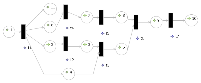
Figure 4: Testcase 1 input, diagram exported from a GMF-based Petri-Net editor.

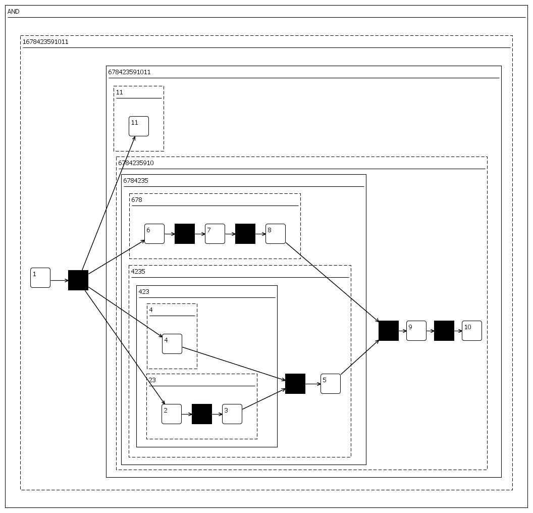
Figure 5: Testcase 1 output, diagram exported from a GMF-based Statechart editor.

4.2 Testcase 2: Insurance Claim Example

This testcase is based on an insurance claim example from a paper at the ER 2012 conference [6]. For that paper, PN2SC is supplemented with pre-processing rules for activity diagrams with object flows. Also, there are post-processing rules for removing hyper-edges and for introducing initial, decision and final nodes in the statecharts. These extensions are not part of the proposed TTC’13 case but we mention them here for clarifying the bigger picture.

Figure 6 shows the input Petri-Net for Testcase 2 while Figure 7 shows the expected output. Similar to Testcase 1, the input Petri-Net should be completely reduced to one place upon transformation termination.

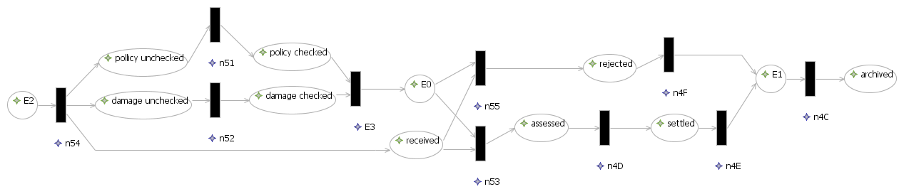
Figure 6: Testcase 2 input, diagram exported from a GMF-based Petri-Net editor.

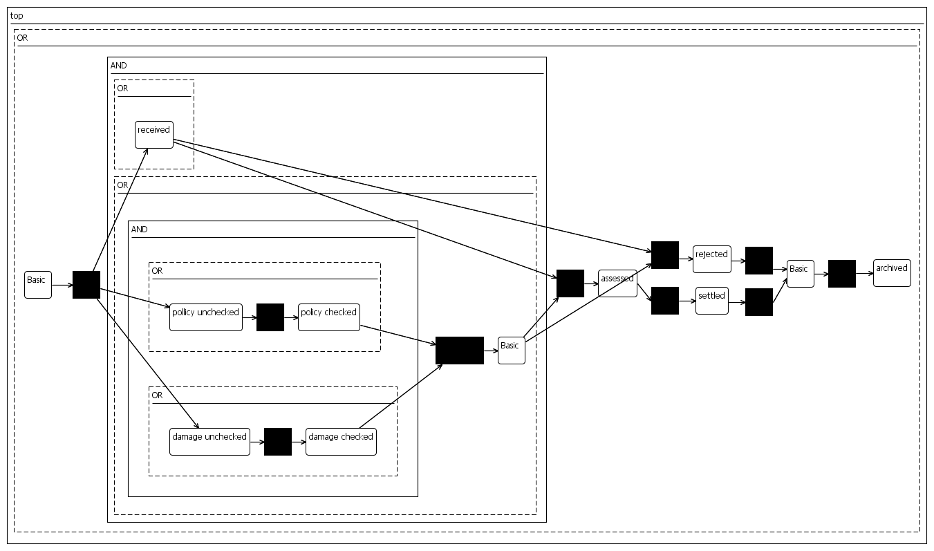
Figure 7: Testcase 2 output, diagram exported from a GMF-based Statechart editor.

4.3 Testcase 3: Patient Logistics Example

This testcase is inspired by the way patients can be routed throughout a hospital in the context of dermatology care. For this testcase, the transformation should terminate in the aforementioned failure state since the input model is not part of the class of Petri-Nets for which the reduction rules have been designed.

Figure 8 shows the input Petri-Net for Testcase 3 as well as a possible visualization of the failed execution. The top of the figure shows the statechart model that was generated so far. Again, OR states are represented as white boxes. There are no AND states in the model, but a gray box is shown nonethless to make the white boxes better visible in print. The bottom of the figure shows the Petri-Net upon transformation failure. The two places (ovals) without labels have been produced by successive applications of the OR reduction rule. The corresponding OR states can be identified at the left and in the middle of the statechart.

Figure 8: Testcase 3 output, diagram exported from the GrGen.NET graph visualizer.

4.4 Performance Testcases

For performance testing, we enclose an EMF representations of the key models that were used to compare the Java and GrGen.NET based solutions of the aforementioned paper by Van Gorp et al. [17]. The models are based on a large Petri-Net that can be transformed successfully by the reduction rules. That Petri-Net has been cloned and merged multiple times to create models of up to 300 thousand elements. All results from [17] can be reproduced via an online virtual machine in SHARE [16]. In general, the performance of both solutions scales linearly for models of normal size (requiring always less than a second.) For models with thousands of elements, the GrGen.NET solution exhibits $\bigcirc(x^{2})$ time complexity.

Figure 9 shows the performance results from a benchmark [17]. The figure shows that for GrGen.NET, two curves are shown. Both curves are based on just one transformation specification. Different results were obtained by changing small engine settings: for one version, the rules are applied directly while for the other version the engine is instructed to first analyze the input model and generate optimized execution code/parameters. The analysis obviously takes time too. It turned out that for models consisting of less than 10.000 elements, the analysis generated too much overhead. The Java solution cannot process more than about 15.000 elements, due to limitations of the address space of the 32 bits Java virtual machine that we have used. For inputs models with more than 10.000 elements, the required processing time increases significantly too. For models of some hundreds of thousands of elements, the engine-provided GrGen optimizations reach a speedup factor of almost two.

Note that our performance tuning and testing of the Epsilon solution described earlier in this paper is not yet complete. Our early results indicate that the Epsilon solution is one or two orders of magnitude slower than the Java solution, which we attribute to a lack of performance tuning, and the interpretative nature of EMF and the Epsilon Object Language.

We encourage case submitters to demonstrate various strategies to performance tuning but point out that for the GrGen.NET solution, the transformation definition (i.e., the rule specification) was not even optimized for performance. In general, especially solutions that deliver good performance without negatively affecting the specification style are considered of high quality.

Measurements taken for the purposes of comparing performance with other solutions must include two intervals: time taken to load / import models and time take to execute the transformation on a model once it has been loaded and imported. To ensure an equitable comparison, measurements must be taken on a SHARE virtual machine image.

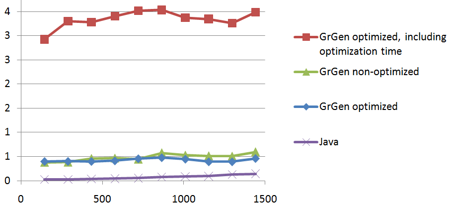
(a)

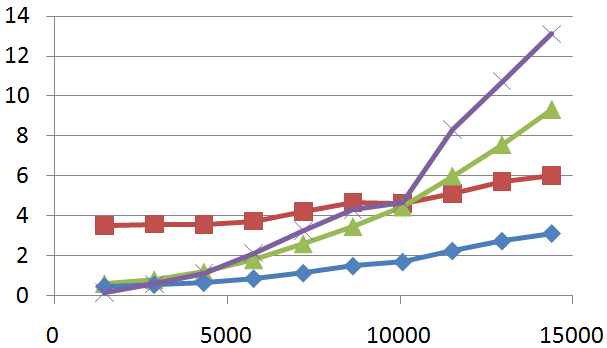
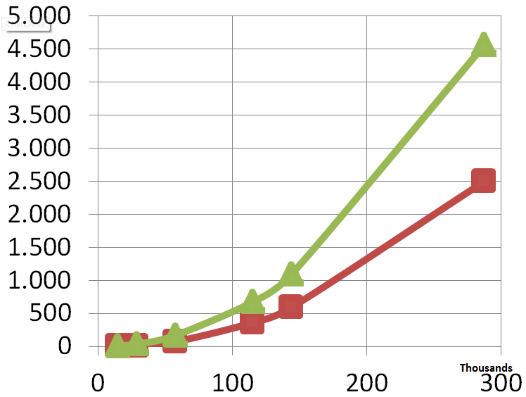
(b)	(c)

Figure 9: Performance (execution time seconds) of Java and GrGen.NET solutions.

4.5 Testcases 4-11: Advanced Control Flows

During the solution discussion phase, we observed the need to share additional testcases. In particular, the testsuite had to be extended with inputs involving more advanced control flow structures. Three weeks before the solution submission deadline, we have shared 8 additional testcases. The additional testcases involve fabricated Petri-Nets that contain advanced Petri-Net synchronization and loop structures. Not all additional petri-nets can be reduced successfully. In summary, input models 1,2, 7, 8 and 11 should be successfully reduced to statecharts while nets 3, 5, 6, 9 and 10 cannot (and should not) be reduced completely.

5 Evaluation Criteria

5.1 Basic Criteria

5.1.1 Transformation Correctness

Solutions should at least demonstrate that they have the intended behavior for all testcases.

5.1.2 Transformation Performance

Secondly, runtime performance should be evaluated (using the performance testcases). An online spreadsheet will be provided for conveniently entering and comparing performance results. Solution submitters are also encouraged to reflect on the good (or poor) performance of their solution, compared to solutions from TTC’13 competitors.

5.1.3 Transformation Understandability

Peer reviews will be used to assess qualitatively the understandability of all solutions. We envision online reviews involving multiple rounds in order to reach consensus among all participants.

5.1.4 Reproducibility

Solution submitters should facilitate the online review by (1) providing an appendix that lists all code, diagrams, scripts, pop-ups that are essential for running the transformation, (2) publishing all artifacts to SHARE. Point (1) ensures that reviewers know where to look while (2) ensures that reviewers can put all artifacts in the proper perspective. For (2), solution submitters are encouraged to provide on the VM desktop one shortcut per testcase. Ideally, clicking such a shortcut automatically demonstrates that the test is passed by the solution. However, this is hard since we do not offer any infrastructure for automatically analyzing whether an output EMF file is the same as the testcase-provided one. Solution submitters who have technology for automating the test procedure are encouraged to share that via the TTC’13 forum. As case proposers, we at least offer the aforementioned GMF editors with an automatic layouting feature for the effective human-based analysis of the generated output models.

5.2 Bonus Criteria

5.2.1 Verification Support

Solution submitters who have technologies to formalize the class of Petri-Nets supported by the reduction rules are encouraged to demonstrate how such technologies should be used effectively. Eshuis has already defined the class of supported nets mathematically [5], but a computer-supported, formal link between the definition of that class and the definition of the reduction rules is missing. Once the definition of the class of supported input models is linked formally to the transformation rules of a solution, it becomes interesting to reason about properties that are satisfied by the set of rules. For example, it would be interesting to have automated analysis features for verifying whether or not the rules terminate for the complete class defined by Eshuis [5]. Similarly, an automated confluence analysis of the rules set would be highly valuable too. It is important that such analyses are applied to classes of input models rather than just to individual inputs. Once automated support for verifying the termination and confluence of a rule set is in place, one can more efficiently experiment with variations to the reduction rules. Finally, note that it would also be useful to reverse the direction of the formal analysis: if it turns out that given a formally defined class of input models $c$, properties $P$ (e.g., termination and confluence) are not satisfied for a set of rules $R$, it would be useful to learn for which subclasses $S$ of $c$ the properties $P$ would be satisfied nonetheless. With the latter type of support in place, it would be interesting to compare the “reverse engineered” formal definition of a maximal subclass against the “manually formalized” class of supported nets that is described in [5].

5.2.2 Simulation Support

Solution submitters are also encouraged to demonstrate features related to the execution of the Petri-Nets and their corresponding statecharts. Note however that execution of the models in isolation is not considered relevant to this case. Instead, we are interested in tools that facilitate for example the simulation of statecharts based on a rule-based Petri-Net simulator (or vice versa).

5.2.3 Transformation Language support for Change Propagation

We are interested in typical scenario’s of change propagation (automatically creating/updating/deleting output model elements when performing updates on a previously transformed input model). To the best of our knowledge, most graph and transformation languages do not yet offer built-in support for this so experts are encouraged to show their unique features for this use case. To facilitate comparison between solutions, we encourage solution developers to address the following change propagation scenarios. However, there may be additional change propagation scenarios that are well-suited to a particular tool and solution developers may also describe these scenarios in addition or instead of the suggestions below.

• Adding a place and a transition in the input Petri-Net should result in a corresponding state and hyper-edge in the output statechart. The arcs should also be updated accordingly. All other elements should remain unchanged. No new AND or OR states should be created.

• Updating the name of a place or transition that was previously transformed should only result in the update of the corresponding statechart element. Furthermore, removing a place (transition) followed by adding a new place (transition) should not be misinterpreted as a renaming operation when propagating changes.

• Removing a place and transition from a sequence in the input Petri-Net should result in the removal of the corresponding state and hyper-edge in the output statechart. The arcs should also be updated accordingly. All other elements should remain unchanged.

Test cases can be provided on request for change propagation scenarios (including but not limited to those listed above).

5.2.4 Transformation Language support for Reversing the Transformation

Previous editions of the TTC did not yet attract convincing solutions based on languages with support for bidirectional transformations. We consider PN2SC a particularly challenging case for such languages since the reduction rules are input-destructive. Therefore, we especially encourage experts in such languages to check whether they can solve the case and also report potentially any negative results.

5.2.5 Transformation Tool support for Debugging

For validation, specialized debuggers tend to offer features for visualizing (input, intermediate and output) models, ideally in the syntax of the corresponding input or output language. Breakpoints can typically be set at the rule level but more fine-grained control can be provided too. Solution submitters are encouraged to document at which level their transformation tool supports breakpoint definition. Also, they are encouraged to document any features they may have employed for turning a generic model/graph/object debugger into a Petri-Net and/or statechart-specific debugger.

5.2.6 Transformation Tool support for Refactoring

Since transformation definitions have to evolve, automated restructuring (refactoring) operations are very relevant but very little transformation tools provide them at the time of writing. This may hinder their adoption compared to general purpose programming languages. Therefore, solution submitters are also encouraged to document any support their tool suite offers for the systematic restructuring of transformation definitions.

6 Table for Comparing Solutions

In order to facilitate the comparison of all submitted results, we encourage solution submitters to document their solution in terms of Table 1. A solution name should distinguish a solution from competing solutions that are based on the same languages or tools (if any). The column “Performance Optimizations” should clarify techniques that were employed for optimizing performance: N indicates that no optimizations were used, M indicates that an optimization algorithm was implemented by hand and E indicates that declarative (engine-provided) optimizations were employed. The table also provides columns for entering the results of the performance tests, as measured within a SHARE VM. The SHARE URL should be provided as a bibtex citation to minimize the size of the table. The column “Understandability” will be based upon the results of the peer reviews, in a qualitative scale (very poor, poor, neutral, good, excellent). Finally the table includes columns for concisely describing the results for bonus criteria. For 5.2.1, C stands for some kind of automatic confluence analysis, T stands for some kind of automatic termination analysis while N stands for no automatic verification support. The specific type of verification support should be elaborated in free text.

Solution

Language

Language

Language

Performance

sp200

sp1000

sp5000

sp10000

sp40000

sp200000

SHARE URL

Understandability

Bonus 5.2.1

Bonus 5.2.2

Bonus 5.2.2

Bonus 5.2.3

Bonus 5.2.4

Bonus 5.2.5

Bonus 5.2.6

Name

for Initialization

for Reduction

for Orchestration

Optimizations

N / M / E

… ms

… ms

… ms

… ms

… ms

… ms

-2 .. +1

C/T/N

Y/N

Y/N

Y/N

Y/N

Y/N

Y/N

Table 1: Table for concisely documenting a solution.

Acknowledgements: The authors thank Prof. Juan de Lara for constructing the initial versions of the Petri-Net and statecharts metamodels used in this case.

References

- [1]
- [2] Marcel van Amstel, Steven Bosems, Ivan Kurtev & Luís Ferreira Pires (2011): Performance in Model Transformations: Experiments with ATL and QVT. In Jordi Cabot & Eelco Visser, editors: Theory and Practice of Model Transformations, Lecture Notes in Computer Science 6707, Springer Berlin / Heidelberg, pp. 198–212, 10.1007/978-3-642-21732-6_14.
- [3] David F. Bacon, Susan L. Graham & Oliver J. Sharp (1994): Compiler transformations for high-performance computing. ACM Comput. Surv. 26(4), pp. 345–420, 10.1145/197405.197406.
- [4] Rik Eshuis (2005): Statecharting Petri Nets. Technical Report Beta WP 153, Eindhoven University of Technology. Available at http://beta.ieis.tue.nl/node/1267.
- [5] Rik Eshuis (2009): Translating Safe Petri Nets to Statecharts in a Structure-Preserving Way. In Ana Cavalcanti & Dennis Dams, editors: FM, LNCS 5850, Springer, pp. 239–255, 10.1007/978-3-642-05089-3_16. Extended as Beta WP 282 at Eindhoven University of Technology.
- [6] Rik Eshuis & Pieter Van Gorp (2012): Synthesizing Object Life Cycles from Business Process Models. In Paolo Atzeni, David W. Cheung & Sudha Ram, editors: ER, Lecture Notes in Computer Science 7532, Springer, pp. 307–320, 10.1007/978-3-642-34002-4_24.
- [7] M. S. Feather (1987): A survey and classification of some program transformation approaches and techniques. In: The IFIP TC2/WG 2.1 Working Conference on Program specification and transformation, North-Holland Publishing Co., Amsterdam, The Netherlands, The Netherlands, pp. 165–195.
- [8] Pieter Van Gorp, Steffen Mazanek & Louis Rose, editors (2011): Proceedings Fifth Transformation Tool Contest. EPTCS 74, 10.4204/EPTCS.74.
- [9] R. Grønmo, B. Møller-Pedersen & G.K. Olsen (2009): Comparison of Three Model Transformation Languages. In: ECMDA-FA’09: European Conference on Model Driven Architecture - Foundations and Applications, LNCS 5562, Springer, pp. 2–17, 10.1007/978-3-642-02674-4_2.
- [10] Niels Lohmann, Eric Verbeek & Remco Dijkman (2009): Petri Net Transformations for Business Processes — A Survey. In Kurt Jensen & Wil M. Aalst, editors: Transactions on Petri Nets and Other Models of Concurrency II, Springer-Verlag, Berlin, Heidelberg, pp. 46–63, 10.1007/978-3-642-00899-3_3.
- [11] Arend Rensink & Pieter Van Gorp (2010): Graph transformation tool contest 2008. International Journal on Software Tools for Technology Transfer (STTT) 12, pp. 171–181, 10.1007/s10009-010-0157-7.
- [12] L.M. Rose, M. Herrmannsdoerfer, J.R. Williams, D.S. Kolovos, K. Garcés, R.F. Paige & F.A.C. Polack (2010): A Comparison of Model Migration Tools. In D.C. Petriu, N. Rouquette & Ø Haugen, editors: MODELS’10: International Conference on Model Driven Engineering Languages and Systems, LNCS 6394, Springer, pp. 61–75, 10.1007/978-3-642-16145-2_5.
- [13] Louis M. Rose, Richard F. Paige, Dimitrios S. Kolovos & Fiona A.C. Polack (2009): An Analysis of Approaches to Model Migration. In: MoDSE-MCCM’09: Joint MoDSE-MCCM Workshop on Models and Evolution, pp. 6–15. Available at http://www.modse.fr/modsemccm09/doku.php?id=Proceedings.
- [14] Gabriele Taentzer, Karsten Ehrig, Esther Guerra, Juan De Lara, Tihamer Levendovszky, Ulrike Prange & Daniel Varro (2005): Model Transformations by Graph Transformations: A Comparative Study. In: Model Transformations in Practice Workshop at MODELS 2005, Montego, p. 05.
- [15] José Barranquero Tolosa, Oscar Sanjuán-Martínez, Vicente García-Díaz, B. Cristina Pelayo G-Bustelo & Juan Manuel Cueva Lovelle (2011): Towards the systematic measurement of ATL transformation models. Softw. Pract. Exper. 41, pp. 789–815, 10.1002/spe.1033.
- [16] Pieter Van Gorp (2013): Online demo: PN2SC in Java and GrGen. http://share20.eu/?page=ConfigureNewSession&vdi=XP_GB9_GrGen_live_AD2HSC_i_i_i_i_i_i_Epsilon_GrGenTTC13_i.vdi.
- [17] Pieter Van Gorp & Rik Eshuis (2010): Transforming process models: executable rewrite rules versus a formalized java program. In: Proceedings of the 13th international conference on Model driven engineering languages and systems: Part II, MODELS’10, Springer-Verlag, Berlin, Heidelberg, pp. 258–272, 10.1007/978-3-642-16129-2_19.
- [18] Dániel Varró, Márk Asztalos, Dénes Bisztray, Artur Boronat, Duc-Hanh Dang, Rubino Geiß, Joel Greenyer, Pieter Van Gorp, Ole Kniemeyer, Anantha Narayanan, Edgars Rencis & Erhard Weinell (2008): Transformation of UML Models to CSP: A Case Study for Graph Transformation Tools. In: AGTiVE’08: International Symposium on Applications of Graph Transformation with Industrial Relevance, LNCS 5088, Springer, pp. 540–565, 10.1007/978-3-540-89020-1_36.