Kaon semileptonic form factors with $N_{f}=2+1+1$ HISQ fermions and physical light quark masses

Abstract:

We present results for the form factor $f_{+}^{K\pi}(0)$, needed to extract the CKM matrix element $|V_{us}|$ from experimental data on semileptonic $K$ decays, on the HISQ $N_{f}=2+1+1$ MILC configurations. The HISQ action is also used for the valence sector. The data set used for our final result includes three different values of the lattice spacing and data at the physical light quark masses. We discuss the error budget and how this calculation improves on our previous determination of $f_{+}^{K\pi}(0)$ on the asqtad $N_{f}=2+1$ MILC configurations.

1 Motivation

A precise determination of the CKM parameter $|V_{us}|$ has been the subject of extensive work using $K$ leptonic and semileptonic decays, as well as hadronic $\tau$ decays. The goal is to test the unitarity of the CKM matrix in the first row and establish stringent constraints on the scale of the new physics that could contribute to these processes [1, 2].

In Ref. [3] we present our result for the $K$ semileptonic form factor $f_{+}(0)$, which includes for the first time data at the physical light quark masses. In this contribution we present further details on the chiral interpolation and continuum extrapolation as well as on our study of the other systematic errors that enter our result. Our result for $f_{+}(0)$ can be used together with experimental data on exclusive semileptonic $K$ decays to extract $|V_{us}|$ with a precision that is currently limited by the uncertainty in $f_{+}(0)$ [4, 5]. The form factor is

$$\langle\pi|V^{\mu}|K\rangle=f_{+}(q^{2})\left[p_{K}^{\mu}+p_{\pi}^{\mu}-\frac{m_{K}^{2}-m_{\pi}^{2}}{q^{2}}q^{\mu}\right]+f_{0}(q^{2})\frac{m_{K}^{2}-m_{\pi}^{2}}{q^{2}}q^{\mu}\,.$$ (1)

The set-up of our calculations is described in Refs. [4] and [6]. We obtain $f_{+}(0)$ from the relation $f_{+}(0)=f_{0}(0)=\frac{m_{s}-m_{l}}{m_{K}^{2}-m_{\pi}^{2}}\langle\pi(p_{\pi})|S|K(p_{K})\rangle$ and simulate directly at zero momentum transfer, $q^{2}\approx 0$, by tuning the external momentum of the $\pi$ using partially twisted boundary conditions. Unlike in our asqtad $N_{f}=2+1$ calculation [4], here we do not include correlation functions with moving $K$’s since they are considerably noisier than with moving $\pi$’s [6].

We use the HISQ action for the sea and valence quarks, simulating on the HISQ $N_{f}=2+1+1$ MILC configurations [7]. We analyze the ensembles listed in Table 1, although we use the ensemble with the smallest lattice spacing, $a\approx 0.06~{}{\rm fm}$, only as a consistency check. The $a\approx 0.12~{}{\rm fm}$ ensemble with $m_{\pi}L=5.36$ is used only for an estimate of finite-volume (FV) effects. In order to avoid autocorrelations, we block our data by four. We try different blocking sizes and find that the results from the correlator fits, both central values and errors, stabilize when the data is blocked by four. We already discussed the correlator fit strategy and the fit functions used in Refs. [4] and [6], so we do not repeat that here. We just show the results for $f_{+}(0)$ for the ensembles we include in our main analysis in Table 2 and in Fig. 1. Statistical (bootstrap) errors are $\sim 0.2$–0.4%. We observe that the variation of the results with lattice spacing is less than the statistical errors, except for the ensemble with $a\approx 0.15~{}{\rm fm}$.

$\approx a$(fm)	$am_{l}^{\rm sea}$	$am_{s}^{\rm sea}$	$am_{c}^{\rm sea}$	$am_{s}^{\rm val}$	$m_{\pi}^{P}$	$m_{\pi}^{{\rm RMS}}$	$L({\rm fm})$	$m_{\pi}L$	$N_{\rm conf}$	$N_{{\rm s}}$
0.15	0.00235	0.0647	0.831	0.06905	133	311	3.2	3.30	$1000$	$4$
0.12	0.0102	0.0509	0.635	0.0535	309	370	3.00	4.54	$1053$	$8$
	0.00507	0.0507	0.628	0.053	215	294	3.93	4.29	$993$	$4$
	0.00507	0.0507	0.628	0.053	215	294	4.95	5.36	$391$	$4$
	0.00184	0.0507	0.628	0.0531	133	241	5.82	3.88	$945$	$8$
0.09	0.0074	0.037	0.440	0.038	312	332	2.95	4.50	$775$	$4$
	0.00363	0.0363	0.430	0.038	215	244	4.33	4.71	$853$	$4$
	0.0012	0.0363	0.432	0.0363	128	173	5.62	3.66	$621$	$4$
0.06	0.0048	0.024	0.286	0.024	319	323	2.94	4.51	$362$	$4$

Table 1: Parameters of the $N_{f}=2+1+1$ gauge-field ensembles used in this work and details of the correlation functions generated. $N_{\rm conf}$ is the number of configurations included in our analysis, $N_{{\rm s}}$ the number of time sources used on each configuration, and $L$ the spatial size of the lattice. $m_{\pi}$’s are given in MeV, where $m^{P}_{\pi}$ is the Goldstone (pseudoscalar taste) $\pi$ mass and $m^{{\rm RMS}}_{\pi}$ the root-mean-squared (over all tastes) $\pi$ mass.

$\approx a({\rm fm})$	$m_{\pi}^{P}\approx m_{\pi}^{{\rm phys}}$	$m_{l}=0.1m_{s}$	$m_{l}=0.2m_{s}$
0.15	0.9744(24)	-	-
0.12	0.9707(18)	0.9808(22)	0.9874(24)
0.09	0.9699(36)	0.9807(22)	0.9868(18)

Table 2: Values of $f_{+}(0)$ included in the chiral interpolation and continuum extrapolation. Errors are statistical only, from 500 bootstrap ensembles.

2 Chiral-continuum interpolation/extrapolation

Although we have data at the physical (and smaller) light-quark masses, we also include data from ensembles with larger light-quark masses in our analysis (see Table 1), and hence use chiral perturbation theory ($\chi$PT) to interpolate to the physical point. This allows us to correct for small mistunings of quark masses and reduce statistical errors. Due to the Ademollo-Gatto (AG) theorem, $f_{+}(0)$ is constrained to follow the chiral expansion $f_{+}(0)=1+f_{2}+f_{4}+f_{6}+\dots$, with $f_{2i}$ chiral corrections of ${\it O}(p^{2i})$ that go to zero in the $SU(3)$ limit as $(m_{K}^{2}-m_{\pi}^{2})^{2}$ up to discretization errors of ${\it O}(\alpha_{S}\texttwosuperior a^{2},a^{4})$ [3]. Following the same strategy as in our asqtad $N_{f}=2+1$ analysis, we use partially quenched staggered $\chi$PT (PQS$\chi$PT) at NLO [8] plus regular continuum $\chi$PT at NNLO [9], and add the discretization effects mentioned above and the dominant $a^{2}$ corrections that respect the AG theorem (other than those included explicitly by the NLO PQS$\chi$PT), i. e., ${\it O}\left((m_{K}^{2}-m_{\pi}^{2})^{2}\alpha_{s}a^{2},(m_{K}^{2}-m_{\pi}^{2})^{2}\alpha_{s}^{2}a^{2}\right)$ terms. We also include isospin corrections at NLO from Ref. [10] and interpolate to the physical $\pi$ and $K$ masses but with electromagnetic effects removed [11, 12], i. e., $m_{\pi^{+}}^{QCD}=135.0~{}{\rm MeV}$, $m_{K^{0}}^{QCD}\approx m_{K^{0}}^{{\rm phys}}=497.7~{}{\rm MeV}$, and $m_{K^{+}}^{QCD}=491.6{\rm MeV}$. $m_{K^{+}}^{\rm QCD}$ above is used only in $f_{2}$, to account for the leading isospin corrections. The fit function is

$$f_{+}(0)=1 + f_{2}^{{\rm PQS\chi PT}}(a)+K_{1}\,\sqrt{r_{1}^{2}a^{2}\bar{\Delta}\left(\frac{a}{r_{1}}\right)^{2}}+K_{3}\,\left(\frac{a}{r_{1}}\right)^{4}+f_{4}^{{\rm cont.}}$$ (2)

$$+ r_{1}^{4}(m_{\pi}^{2}-m_{K}^{2})^{2}\left[\,C_{6}+K_{2}\,\sqrt{r_{1}^{2}a^{2}\bar{\Delta}\left(\frac{a}{r_{1}}\right)^{2}}+K_{2}^{\prime}\,r_{1}\texttwosuperior a^{2}\bar{\Delta}\right]\,,$$

where the constants $K_{i}$ and $C_{i}$ are fit parameters to be determined by the chiral fits using Bayesian techniques , $\bar{\Delta}$ is the average taste splitting $\bar{\Delta}=\frac{1}{16}\left(\Delta_{P}+4\Delta_{A}+6\Delta_{T}+4\Delta_{V}+\Delta_{I}\right)$, and $r_{1}^{2}a^{2}\bar{\Delta}$ is a proxy for $\alpha_{s}^{2}a^{2}$. $C_{6}$ is proportional to the combination of low-energy constants (LEC’s) $C_{12}+C_{34}-L_{5}^{2}$ [13], where $C_{ij}$ are ${\it O}(p^{6})$ and $L_{5}$ is ${\it O}(p^{4})$. We follow the same approach as in Ref. [4] and take the ${\it O}(p^{4})$ LEC’s and the taste-violating hairpin parameters [15] as constrained fit parameters. The corresponding uncertainties are thus included in the error of the central value. The HISQ taste splittings, which we take from Ref. [7], are known precisely enough that their error has no impact on the final uncertainty. The prior central values and widths we use in our fits are in Table 3.

Table 3: Priors (central value$\pm$width) for the fit parameters entering in Eq. (2.1). The $\chi$PT parameter $s$ is given by $1/(16\pi^{2}(r_{1}f_{\pi})^{2})$. The priors listed for the hairpin parameters are for the $a\approx 0.12~{}{\rm fm}$ ensembles, and those for the other lattice spacings are obtained by rescaling this number, assuming that the hairpin parameters scale like the $\Delta_{\Xi}$. The central values for the NLO LEC’s $L_{i}^{\prime}s$ are from fit 10 in Ref. [14].

$r_{1}^{2}a^{2}\delta_{V}^{{\rm HISQ}}$	$r_{1}^{2}a^{2}\delta_{A}^{{\rm HISQ}}$	$K_{1}$	$K_{2}$	$K_{2}^{\prime}$	$K_{3}$	$C_{2i}$
$0.057\pm 0.033$	$-0.0782\pm 0.0040$	$0\pm 0.01$	$0\pm 0.03$	$0\pm 0.081$	$0\pm 0.015$	$0\pm s^{i-1}$

$L_{1}^{r}(M_{\rho})$	$L_{2}^{r}(M_{\rho})$	$L_{3}^{r}(M_{\rho})$	$L_{4}^{r}(M_{\rho})$	$L_{5}^{r}(M_{\rho})$
$0.43\pm 0.24$	$0.73\pm 0.24$	$-2.30\pm 0.74$	$0.0\pm 0.6$	$0.97\pm 0.22$

$(2L_{6}^{r}-L_{4}^{r})(M_{\rho})$	$L_{7}^{r}(M_{\rho})$	$L_{8}^{r}(M_{\rho})$
$0.0\pm 0.4$	$-0.31\pm 0.28$	$0.60\pm 0.36$

With the fit function in Eq. (2) and including the data at $a\approx 0.15,0.12,0.09~{}{\rm fm}$ in Table 1 we get $f_{+}(0)=0.9703(23)$. The interpolation as well as the data points included in the fit and those used for estimating systematic errors or as a consistency check, are shown in Fig. 1.

2.1 Systematic error analysis

As explained in Ref. [3], we expect that the error in our chiral-continuum fit value includes both statistical and discretization errors. In order to check this expectation, we also follow an alternate strategy to try to separate statistical from discretization errors. The central value for this second strategy is given by a fit that does not include any extra $a^{2}$ terms (besides those in the one-loop S$\chi$PT expression), but without including the $a\approx 0.15~{}{\rm fm}$ point, $f_{+}(0)=0.9708(15)$. Then we perform a number of fits using fit functions in which we parametrize discretization errors in different ways, including all possible combinations of the four terms in Eq. (2) and continuum NNLO $\chi$PT plus analytic $a^{2}$, $\alpha_{s}a^{2}$, and $a^{4}$ terms. The different parametrizations do not move the central value more than 0.0010, well below the statistical error. If we take this variation as the estimate of discretization errors for this alternate fit strategy, we obtain a combined statistical and discretization error of $\pm 0.0018$, which is smaller than the corresponding error for our central result.

The chiral interpolation is very much constrained by the data at the physical light quark masses, so the dependence of the fit result on the $\chi$PT parameters is very much suppressed. For example, we can test the choice of fit function by using an analytic parametrization instead of the continuum two-loop ChPT expression. The results from NNLO, N³LO, and N⁴LO analytic parametrizations agree with our central value well within statistical errors.

A more accurate test of higher order effects in the chiral expansion is achieved by adding N³LO, and N⁴LO analytic terms to the fit function. Adding an N³LO term $C_{8}\,(m_{K}^{2}-m_{\pi}^{2})^{2}m_{\pi}^{2}$ to Eq. (2) with an unknown but constrained coefficient slightly changes the central value to 0.9704 and increases the error to 0.0024  When, in addition, we add a $N^{4}LO$ term, $C_{10}\,(m_{K}^{2}-m_{\pi}^{2})^{2}m_{\pi}^{4}$, the central value and error do not change. In other words, the result from the chiral and continuum fit stabilizes once we include up to $N^{3}LO$ chiral corrections. We thus take the result from that fit, $f_{+}(0)=0.9704(24)$, as our central value for the form factor and the error including statistics, discretization effects, and higher order chiral corrections.

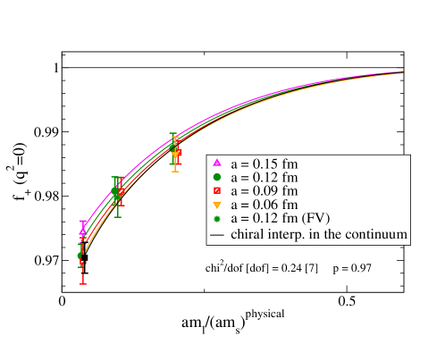
Figure 1: Form factor $f_{+}(0)$ vs. light-quark mass. Errors shown on the data points are statistical only, obtained from 500 bootstrap ensembles. Different symbols and colors denote different lattice spacings, and the corresponding colored lines show the chiral interpolation at fixed lattice spacing. The green star labels the ensemble we use to estimate FV effects. The solid black line is the interpolation in the light-quark mass, keeping $m_{s}$ equal to its physical value, and turning off all discretization effects.

We have, however, another systematic effect arising from the fact that for some ensembles we have different strange-quark masses in the sea and in the valence sectors. This difference is treated correctly at NLO, since we have a partially quenched S$\chi$PT fit function, but at NNLO the continuum expression is only evaluated for the full QCD case, with no difference between the sea and valence sectors. We use $m_{s}^{\rm val}$ in the NNLO piece, $f_{4}$, for our central result. But, in order to estimate the uncertainty associated with this choice, we redo the fit replacing $m_{s}^{{\rm val}}$ by $m_{s}^{{\rm sea}}$ in $f_{4}$ except in the overall factor $(m_{K}\texttwosuperior-m_{\pi}^{2})^{2}$ which is generated by the valence sector. The shift in $f_{+}(0)$ is 0.0003 for our main analysis, which we take as the associated systematic error.

Finite volume effects can be systematically addressed in the framework of $\chi$PT, replacing the infinite volume integrals by FV ones and extrapolating to the infinite volume limit. The S$\chi$PT incorporating these effects for our calculation of $f_{+}(0)$ with partially twisted boundary conditions is not yet available, although work is in progress [16]. In order to estimate the FV error, we perform two tests. We carried out an additional simulation on an ensemble with the same parameters as the $a\approx 0.12~{}{\rm fm}$, $m_{l}=0.1m_{s}$ but with a larger volume (fourth line in Table 1 and open circle in Fig. 1). This larger volume simulation gives a result $\sim 0.1\%$ lower, or about half of the smaller of the two statistical errors of the ensembles we are comparing. We check the stability of this shift by performing a variety of correlator fits with different parameters without finding a larger effect. We also perform a second test in which we replace the logarithmic functions and their derivatives in the NLO chiral expression by their FV counterparts [17], $\textrm{ln}\frac{m^{2}}{\Lambda^{2}}\rightarrow\left(\textrm{ln}\frac{m^{2}}{\Lambda^{2}}+\delta_{1}(mL)\right)$ and $-\left(\textrm{ln}\frac{m^{2}}{\Lambda^{2}}+1\right)\rightarrow-\left(\textrm{ln}\frac{m^{2}}{\Lambda^{2}}+1\right)+\delta_{3}(mL)$, and redo the chiral interpolation and continuum (+infinite volume) extrapolation. With this replacement $f_{+}(0)$ decreases by $0.11\%$. This test does not take into account all the possible FV corrections or the fact that we are using twisted boundary conditions (which modifies the FV integrals), but it gives us an idea of the size of these corrections. We take the full size of the statistical error of the $a\approx 0.12~{}{\rm fm}$, $m_{l}=0.1m_{s}$ ensemble, $0.2\%$, as our FV error estimate. We consider the effect of the scale uncertainty on the dimensionless quantity $f_{+}(0)$. Here we use $r_{1}=0.3117\pm 0.0022~{}{\rm fm}$ from Ref. [18], which yields an error of $\pm 0.0008$ on $f_{+}(0)$. Finally, for the estimate of the higher order isospin corrections in the $K^{0}\pi^{+}$ mode, we take twice the difference between the isospin-conserving and isospin-violating calculation of $f_{+}(0)$ at NNLO from Ref. [19].

3 Conclusions

Our final result for the vector form factor is

$$f_{+}(0)=0.9704(24)(22)=0.9704(32)\,,$$ (3)

where the first error in the middle is the combined statistical, discretization, and chiral interpolation error, and the second is the sum in quadrature of the other systematic errors discussed above. Combining the two in quadrature again yields the error on the right. We discuss the implications of this result for the unitarity of the CKM matrix in Ref. [3].

The alternate fit strategy in which we try to disentangle statistical and discretization errors, estimating the other systematic errors in the same way we do for our main strategy gives the result: $f_{+}(0)=0.9708(15)(24)=0.9708(28)$, where the first error is statistical plus higher order terms in the chiral expansion, and the second the remainder of the systematic errors, including discretization effects. The total error of this second strategy is slightly smaller than the one in our main analysis, which confirms the robustness of our systematic error analysis.

We also perform a combined analysis of our HISQ $N_{f}=2+1+1$ data and the asqtad $N_{f}=2+1$ data analyzed in Ref. [4]. We use the fit function in Eq. (2) plus N³LO and N⁴LO chiral corrections and the one in Eq. (4.2) of Ref. [4] (again, plus N³LO and N⁴LO chiral corrections) for the HISQ on HISQ and HISQ on asqtad data, respectively. Notice that $f_{2}^{PQS\chi PT}(a)$ is different for the two sets of data, since the current analysis uses the HISQ action for both the sea and the valence quarks while the asqtad one is a mixed-action calculation with asqtad quarks in the sea and HISQ in the valence sector. The $PQS\chi PT$ expressions, which can be found for both cases in Ref. [8], take into account the differences between valence and sea as well as the particularities of the specific staggered action used. Among other parameters, the continuum LEC’s and the coefficients $C_{2i}$ are the same for all data. Our combined fit provides an average of the two results taking into account correlations in a proper way. The result is $f_{+}(0)=0.9686(17)(14)(6)(20)(2)=0.9686(30)\,$, where the first error is, again, the statistical+discretization+higher order chiral corrections error, the second one is from the mistuning of $m_{s}$ in the sea, the third reflects the uncertainty in $r_{1}$, the fourth is our estimate of FV corrections, and the last higher order isospin effects. The errors are estimated in the same way as described in Sec. 2.1 above.

The result presented here and in Ref. [3] already constitutes the most precise determination of the vector form factor $f_{+}(0)$ and the first one to include simulations directly at the physical light-quark masses. However, to match the experimental uncertainty, we need to reduce the uncertainty on $f_{+}(0)$ further. Work is therefore continuing to address the two main sources of uncertainty in our result, statistics and FV effects. On one hand, there is an ongoing calculation of FV corrections at one-loop in S$\chi$PT [16] which will allow us to eliminate part of this uncertainty and do a more reliable estimate of the remaining effect. On the other hand, there are already more configurations in the ensembles that we have analyzed and new ensembles that we plan to include in future work. Especially important will be to reduce the statistical errors in the physical quark mass $a\approx 0.09~{}{\rm fm}$ ensemble and to add an even finer lattice spacing at $a\approx 0.06~{}{\rm fm}$, also with physical masses.

References

- [1] M. Antonelli et al., Eur. Phys. J. C69, 399-424 (2010). [arXiv:1005.2323 [hep-ph]].
- [2] V. Cirigliano, J. Jenkins and M. Gonzalez-Alonso, Nucl. Phys. B 830 (2010) 95 [arXiv:0908.1754 [hep-ph]].
- [3] A. Bazavov et al., in preparation.
- [4] A. Bazavov et al., Phys. Rev. D 87, 073012 (2013) [arXiv:1212.4993 [hep-lat]].
- [5] V. Lubicz et al. [ETM Collaboration], Phys. Rev. D 80 (2009) 111502 [arXiv:0906.4728 [hep-lat]]; P. A. Boyle et al. [RBC-UKQCD Collaboration], Eur. Phys. J. C 69 (2010) 159 [arXiv:1004.0886 [hep-lat]]; T. Kaneko et al. [JLQCD Collaboration], PoS LATTICE 2012, 111 (2012) [arXiv:1211.6180 [hep-lat]]; P. A. Boyle, J. M. Flynn, N. Garron, A. Jüttner, C. T. Sachrajda, K. Sivalingam and J. M. Zanotti, JHEP 1308, 132 (2013) [arXiv:1305.7217 [hep-lat]].
- [6] E. Gámiz et al., PoS LATTICE 2012, 113 (2012) [arXiv:1211.0751 [hep-lat]].
- [7] A. Bazavov et al. [MILC Collaboration], Phys. Rev. D 87, 054505 (2013) [arXiv:1212.4768 [hep-lat]].
- [8] C. Bernard, J. Bijnens and E. Gámiz, arXiv:1311.7511 [hep-lat].
- [9] J. Bijnens, P. Talavera, Nucl. Phys. B669 (2003) 341-362. [hep-ph/0303103].
- [10] J. Gasser and H. Leutwyler, Nucl. Phys. B 250, 517 (1985).
- [11] S. Aoki et al., arXiv:1310.8555 [hep-lat].
- [12] S. Basak et al. [MILC Collaboration], PoS CD 12, 030 (2013) [arXiv:1301.7137 [hep-lat]].
- [13] J. Bijnens, G. Colangelo and G. Ecker, JHEP 9902, 020 (1999) [hep-ph/9902437].
- [14] G. Amorós, J. Bijnens and P. Talavera, Nucl. Phys. B 602 (2001) 87 [hep-ph/0101127].
- [15] A. Bazavov et al. [MILC Collaboration], PoS LATTICE 2011, 107 (2011) [arXiv:1111.4314], and work in progress.
- [16] C. Bernard, J. Bijnens and E. Gámiz, in preparation.
- [17] C. Bernard [MILC Collaboration], Phys. Rev. D 65, 054031 (2002) [hep-lat/0111051].
- [18] A. Bazavov et al. [Fermilab Lattice and MILC Collaborations], Phys. Rev. D 85, 114506 (2012) [arXiv:1112.3051 [hep-lat]].
- [19] J. Bijnens and K. Ghorbani, arXiv:0711.0148 [hep-ph].