Anisotropic optical conductivity and electron-hole asymmetry in doped monolayer graphene in the presence of the Rashba coupling

Abstract

In this study, the Optical conductivity of substitutionary doped graphene is investigated in presence of the Rashba spin orbit coupling (RSOC). Calculations have been performed within the coherent potential approximation (CPA) beyond the Dirac cone approximation. Results of the current study demonstrate that the optical conductivity is increased by increasing the RSOC strength. Meanwhile it was observed that the anisotropy of the band energy results in a considerable anisotropic optical conductivity (AOC) in monolayer graphene. The sign and magnitude of this anisotropic conductivity was shown to be controlled by the external field frequency. It was also shown that the Rashba interaction results in electron-hole asymmetry in monolayer graphene.

1 Introduction

Recently graphene has attracted a rapidly growing interest due to its potential application in nano-electronics [1, 2]. The extremely high mobility of graphene, in comparison with conventional semiconductors, constitutes a natural outstanding candidate to design high performance electronic devices for next generation electronics. Due to these surprising features of graphene, the coming years has been named as carbon new age [3]. However lack of an energy gap in graphene is one of the biggest hurdles for graphene device applications [4].
The effect of Spin orbit coupling (SOC) on the monolayer graphene was found firstly by Kane and Mele [5, 6]. Strength of intrinsic spin orbit coupling (ISOC) in comparison with the RSOC is very small [7, 8, 9, 10, 11, 12]. Meanwhile the RSOC strength in graphene has been reported up to 0.2eV [13] where can be considered as a really high value for a typical spin-orbit interaction.
The RSOC has been observed by impurity doping and external electric field where the strength of doping induced RSOC is very weak [14]. Meanwhile, it was shown that the RSOC can open and control a noticeable gap at the Dirac points [8, 15].
The effect of the RSOC on heavy doped graphene has been investigated in [16]. The effect of the impurities has been considered by choosing chemical potential close to the M point in the first Brillouin zone (BZ) [16]. Results of this research show that the RSOC in mono-layer graphene can strongly affect the optical response of graphene [16].
In the present study we formulated the effect of the impurities on the optical conductivity of the mono-layer graphene in the presence of RSOC. Numerical calculations have been performed under the coherent potential approximation (CPA) where we have shown that the density of states and the transition rate can be effectively controlled by the density of impurities. It was shown that the RSOC removes the electron-hole band symmetry. In this way we have to consider the deformation of the band energies and density of states as result of the impurities.
Owning to the fact that the RSOC Hamiltonian is translationally invariant, it can be formulated under CPA approach as shown in later sections. The CPA is one of the important and widely used method for describing disordered systems. The problem is that how conductivity of disordered graphene can be affected by the RSOC under CPA approach?
In this manuscript, band structure of graphene has been studied beyond the Dirac cone approximation in framework of tight-binding Hamiltonian. As a result, trigonal warping (TW) of the energy bands can contribute in optical conductivity. The TW is observed when Fermi circle of a degeneracy point lead to deformation [17] by increasing the Fermi energy. TW was expected to be responsible for anisotropic optical conductivity (AOC) as it removes isotropic band cross sections at Fermi level, however the results of the current study show that, even at low Fermi energies i.e. when the TW is negligible the amount of the AOC is really significant. Dirac-cone approximation suppresses the TW effect and therefore the intrinsic anisotropy of the bands (regardless of the position of the Fermi energy) can be responsible for AOC of single layer graphene. It seems that the TW could produce some kind of anisotropic effects when, only the occupied states are allowed to contribute in this process. Meanwhile it should be noted that in some of the physical processes such as optical absorption, where a transition is required between an occupied and another empty state. The anisotropy of the entire band energies could result in AOC. The effect of the RSOC on the AOC of a monolayer graphene has also been studied in the current work. The AOC manifests itself when the the optical conductivity was different along $x$ and $y$ directions.
Electron density of state (DOS), the optical conductivity of graphene can be controlled by manipulating gate voltage which controlls the RSOC strength. Optical properties of a pure monolayer graphene has been studied in [18]. Where it was shown that RSOC can result in a controllable blue shift. In the present work, Density of state, AOC of disordered graphene calculated beyond the Dirac-cone approximation.

2 Theoretical model

In the current work we have considered a monolayer graphene, in which its two-dimensional lattice has been oriented with respect to the $x$ and $y$ axis as shown in Fig. 1.
Nearest neighbor-tight binding Hamiltonian of pure graphene reads

$$H_{0}=-t\sum_{<i,j>,\sigma}\,({{a}^{\dagger}}_{\sigma,i}{{b}_{\sigma,j}}+h.c)$$ (1)

Where the operators $a_{\sigma,i}^{\dagger}$ and ${{b}_{\sigma,j}}$ denote the creation and annihilation of an electron with spin ${\sigma}$ in sublattices A and B (Fig. 1), respectively. Where $t=2.66$ eV is hopping parameter.
RSOC can generate a gap in graphene and converts graphene to semiconductor. According to the results of density functional theory and other approaches, the strength of the ISOC is several orders of magnitude weaker than the strength of RSOC (the strength of ISOC is about 1-50$\mu$eV) [7, 8, 9, 10, 11, 12, 13]. Therefore in this paper the effect of ISOC ( also ISOC in next nearest neighbor) is neglected.
RSOC in graphene and other structures emerges when lattice inversion symmetry is broken [19]. In this study RSOC can be considered to be induced by perpendicular gate voltage or by coupling with the substrate. Rashba coupling is given in the form of a nearest neighbor hopping term as follows [14]

$${{H}_{R}}=-{{t}_{R}}\sum_{<i,j>}\,c_{i}^{\dagger}(\textbf{s}\times\hat{{{d}_{{ij}}}}).{\mathop{{\hat{z}}{{{c}}_{j}}}}\,+h.c.$$ (2)

s is the vector of Pauli matrices, $\hat{{{d}_{{ij}}}}$ is the unit vector that connects the i and j lattice sites and $t_{R}$ is the strength of RSOC where $<i,j>$ indicates that the sum is performed over the nearest neighbors (Fig. 1).
Matrix representation of total Hamiltonian on wave function $\psi=({{\psi}_{A\uparrow}},{{\psi}_{A\downarrow}},{{\psi}_{B\uparrow}},{{\psi}_{B\downarrow}})$ is given by

$$\,{{H}_{0}}=\left(\begin{array}[]{llll}0&0&\gamma(\textbf{k})&0\\ 0&0&0&\gamma(\textbf{k})\\ \gamma^{*}(\textbf{k})&0&0&0\\ 0&\gamma^{*}(\textbf{k})&0&0\end{array}\right),$$ (7)

and

$$\,{{H}_{R}}=\left(\begin{array}[]{llll}0&0&0&\beta_{+}(\textbf{k})\\ 0&0&\beta_{-}(\textbf{k})&0\\ 0&\beta_{-}^{*}(\textbf{k})&0&0\\ \beta_{+}^{*}(\textbf{k})&0&0&0\end{array}\right).$$ (12)

where $\gamma(\textbf{k})={{e}^{-ia{{k}_{y}}}}+2{{e}^{-i\frac{a}{2}{{k}_{y}}}}\cos({{a}_{1}}{{k}_{x}})$ ${{\beta}_{\pm}}=i\,{{t}_{R}}({{\xi}_{1}}(k)\pm{{\xi}_{2}}(k))$, ${{\xi}_{1}}(k)={{e}^{i{{a}_{1}}{{k}_{x}}}}({{e}^{-i{{a}_{2}}{{k}_{y}}}}-\cos({{a}_{1}}{{k}_{x}}))$ and ${{\xi}_{2}}(k)=\sqrt{3}{{e}^{i{{a}_{1}}{{k}_{x}}}}\sin({{a}_{1}}{{k}_{x}})$ in which ${{a}_{1}}=\frac{\sqrt{3}a}{2},\,{{a}_{2}}=\frac{3}{2}a$ in which the carbon-carbon distance is denoted by $a=1.42$Å.
Using the perturbation theory we can obtain the eigenstates of $H_{0}+H_{R}$ as follows

$$\left|{1k}\right\rangle=\left(\begin{array}[]{l}1\\ 0\\ -\varphi_{k}^{*}\\ \varphi_{k}^{*}\\ \end{array}\right),~{}~{}~{}\left|{2k}\right\rangle=\left(\begin{array}[]{l}0\\ 1\\ \varphi_{k}^{*}\\ -\varphi_{k}^{*}\\ \end{array}\right),$$ (21)

$$\left|{3k}\right\rangle=\left(\begin{array}[]{l}-{\varphi_{k}}\\ {\varphi_{k}}\\ 1\\ 0\\ \end{array}\right),~{}~{}~{}\left|{4k}\right\rangle=\left(\begin{array}[]{l}{\varphi_{k}}\\ -{\varphi_{k}}\\ 0\\ 1\\ \end{array}\right),$$ (30)

where we have defined $\varphi_{k}={{x}_{k}}/({4{{\left|\gamma_{k}\right|}^{2}}}),\,\,\,\,{{x}_{k}}=\gamma_{k}\beta_{-}^{*}-{{\gamma_{k}}^{*}}{{\beta}_{+}}$.
Where each state corresponds to the following eigenvalues

$$E_{1,k}=-\left|\gamma_{k}\right|-4\left|\gamma_{k}\right|\,{{\left|\varphi_{k}\right|}^{2}}\,\,\,,\,\,\,E_{2,k}=-\left|\gamma_{k}\right|-4\left|\gamma_{k}\right|\,{{\left|\varphi_{k}\right|}^{2}}$$ (31)

$$E_{3,k}=\left|\gamma_{k}\right|+4\left|\gamma_{k}\right|\,{{\left|\varphi_{k}\right|}^{2}}\,\,\,\,,\,\,\,\,E_{4,k}=\left|\gamma_{k}\right|+4\left|\gamma_{k}\right|\,{{\left|\varphi_{k}\right|}^{2}}$$ (32)

It should be noted that the exact expression for these eigenstates and eigenvalues are also available however, we have observed that the use of these compact form of the eigenstates and eigenvalues, given by the perturbation theory, results in a significant time saving during the self consistent computations.
Under of CPA theory Hamiltonian of electron in this system is $H=H_{0}+H_{R}+V$ which $V$ is the short range potential arising from the substitutional impurities. The Green’s function of pure system, ${G}_{0}$, is given by

$${{G}_{0}}(z)=\frac{1}{z-{{H}_{0}}-H_{R}}$$ (33)

In the CPA approach the Hamiltonian is given by

$$H=H_{0}+H_{R}+\Sigma+V-\Sigma$$ (34)

The site dependent self energies $\Sigma(E)$ should be determined during the CPA algorithm. By using a self-consistent approach one can obtain as much as possible accurate self-energies using the following relations

$$G_{eff}={{G}}+{{G}}V^{\prime}G_{eff}.$$ (35)

In which we have defined

$$V^{\prime} = V-\Sigma(E)$$ (36)

$${{G}}(z) = \frac{1}{z-{{H_{eff}}}}$$ (37)

$$H_{eff}(E) = H_{0}+H_{R}+\Sigma(E).$$ (38)

Equation (35) can be restated in term of the $T$-Matrix formalism as follows

$$G_{eff} = {{G}}+{{G}}T{{G}},$$ (39)

$$T = V^{\prime}+V^{\prime}GT.$$ (40)

The effective self energies can be determined if the following condition is satisfied

$$<G_{eff}>={{G}},$$ (41)

i.e. when

$$<T>=0.$$ (42)

In which $<>$ denotes the configurational averaging.
When we applied self-consistency to average T-matrix, finally site independent self-energy of effective medium achieved. The CPA self-consistent equations in the unit cell may be restated as

$$\Sigma_{\lambda,A/B}(z)=(x/2){{\varepsilon}_{A/B}}+(1-x/2){{\varepsilon}_{A/B}}-({{\varepsilon}_{A/B}}-\Sigma_{\lambda}){{\bar{G}}^{\lambda}_{00}}({{\varepsilon}_{A/B}}-\Sigma_{\lambda})$$ (43)

Which ${{\bar{G}}_{00}}(z)$ trace of all configurations in real space.

$${{\bar{G}}^{\lambda}_{00}}(z)=\frac{1}{{{\Omega}_{1BZ}}}\int\limits_{1BZ}{\frac{d{{k}_{x}}d{{k}_{y}}}{(z-E_{\lambda}(k)-\Sigma_{\lambda})}},$$ (44)

this integration is over the entire range of the first Brillouin zone. Therefore using the Dirac point approximation in $E_{\lambda}(k)$ gives incorrect results. Consequently the Dirac point approximation cannot be employed in the CPA approach. In the above expressions $z=E+i\epsilon$ where $\epsilon$ is infinitesimally small positive number. $A$, $B$ referred to the different sublattices of the graphene and $x$ is the density of impurities. Since $A$ and $B$ sublattices can be treated on the same footing we can write $\Sigma_{\lambda,A}=\Sigma_{\lambda,B}$ and the density of impurities on each sublattice will be identical and therefore given by $x/2$.
We have employed a diagonal self energy matrix as follows [20]

$$\,{{\Sigma}}=\left(\begin{array}[]{llll}\Sigma_{1}(E)&0&0&0\\ 0&\Sigma_{2}(E)&0&0\\ 0&0&\Sigma_{3}(E)&0\\ 0&0&0&\Sigma_{4}(E)\end{array}\right),$$ (49)

When the self energies is finally obtained. Density of state in term of Green’s function is expressed as

$${D(E)}=-\frac{1}{\pi}{TrIm}<G(E)>$$ (50)

3 Optical conductivity

Real part of conductivity in Linear response theory for disordered systems at arbitrary incident energy, $\omega$, given in term of Kobu-GreenWood equation [21, 22]

$$\sigma_{1x_{i}x_{j}}\left(\omega\right)=\frac{e^{2}\hbar}{S\pi}\int\frac{f\left(E\right)-f\left(E+\hbar\omega\ \right)}{\hbar\omega}dE~{}Tr\{{{v}_{x_{i}}}{ImG}(E+\hbar\omega){{v}_{x_{j}}}ImG(E)\}$$ (51)

$f(E)$ is Fermi-Dirac distribution, $v_{x_{i}}$ is velocity of electron in $x_{i}$ direction and $S$ is surface of our system we have ${{v}_{x_{i}}}=dx_{i}/dt=(i/\hbar)[H_{0}+H_{R},\,x_{i}]$. Since $G_{eff}(E)$ is diagonal in k-space representation, vertex correction cannot be captured in this method. We can write

$$\sigma_{1x_{i}x_{j}}(\omega) = \frac{\hbar{{e}^{2}}}{\pi\Omega}\int{dE\frac{f(E)-f(E+\hbar\omega)}{\hbar\omega}}$$

$$\times\sum_{\eta{\eta}^{\prime}}\sum_{k{k}^{\prime}}\left|\left\langle\eta k|\left.{{v}_{x}}\right|{\eta}^{\prime}{k}^{\prime}\right\rangle\right|^{2}{Im}{{G}_{{\eta}^{\prime}{k}^{\prime}}}(E+\hbar\omega){Im}{{G}_{\eta k}}(E).$$

In which

$$\left\langle\eta k|\left.{{v}_{x}}\,\right|{\eta}^{\prime}{k}^{\prime}\right\rangle = \frac{i}{S\hbar}\int{{{e}^{i({k}^{\prime}-k).\vec{r}}}\,x\,dr}({{E}_{\eta k}}-{{E}_{{\eta}^{\prime}{k}^{\prime}}})\left\langle\eta|{{\eta}^{\prime}}\right\rangle$$ (53)

$${{\left|\left\langle\eta k|\left.{{v}_{x}}\,\right|{\eta}^{\prime}{k}^{\prime}\right\rangle\right|}^{2}} = \frac{1}{{{\hbar}^{2}}}\frac{{{({{E}_{\eta k}}-{{E}_{{\eta}^{\prime}{k}^{\prime}}})}^{2}}}{{{\left|{{{{k}^{\prime}}}_{x}}-{{k}_{x}}\right|}^{2}}}{{\delta}_{{{k}_{y}}\,{{{{k}^{\prime}}}_{y}}}}{{\left|\left\langle{{\eta}^{\prime}}|\eta\right\rangle\right|}^{2}}.$$ (54)

Similarly imaginary part of the Green’s function is given by

$${Im}\,{{G}_{\eta k}}(E)=\frac{{Im}\,{{\Sigma}_{\eta}}}{{{(E-{{E}_{\eta k}}-{Re}\,{{\Sigma}_{\eta}})}^{2}}+{{({Im}\,{{\Sigma}_{\eta}})}^{2}}}$$ (55)

Finally the AOC can be obtained by

$$AOC=\frac{\sigma_{xx}-\sigma_{yy}}{\sigma_{xx}+\sigma_{yy}}$$ (56)

4 Results and discussions

The results of the current study show that substrate induced spin-orbit coupling could change the density of states and the gap energy, introduced by the impurities Figs 2-3. Therefore presence of the impurities in the graphene, results in some additional effects other than the change in Fermi energy. Meanwhile it should be noted that increasing the Rashba coupling removes the electron-hole symmetry as shown in the Fig. 3. It can be inferred by comparison of the Figs 2-3 that in the absence of the Rashba interaction, single layer graphene has a symmetric density of states in both $E>0$ and $E<0$ ranges of energy and substitutional impurities can not remove this symmetry, however when we switch on the Rashba coupling a significant electron hole asymmetry arises Figs 2-3.
The effect of the RSOC on the optical conductivity of doped graphene has been shown for different Rashba coupling strengths Fig. 4. Since splitting of the band energies is effectively increased by Rashba coupling the blue shift of the absorption curve is expected by increasing the Rashba coupling. These results confirms that, increasing the Rashba coupling strength, simultaneously increases and shifts the real part of the optical conductivity in doped graphene. This is in agreement with the results of the Rashba coupling induced blue shift in the pure graphene.
Another interesting feature of the obtained results is the considerable AOC in the monolayer graphene as shown Fig. 5. Numerical results show that the optical conductivity (and therefore optical absorption)is highly dependent on the direction of the external field polarization, where the sign and amount of this anisotropy is determined by the frequency of the external field (Fig. 5). The RSOC can slightly modify the AOC of the doped graphene at any given frequency, however AOC mainly depends on our approach which has been performed beyond the Dirac point approximation.
At the level of the Dirac point approximation we would get a fully symmetric circle shaped of the Fermi surfaces centered at each Brillouin zone corner. Since the absorption process and any scattering process could take place mainly between the occupied and empty states. Therefore the whole Brillouin zone could contribute into the photon absorption. Accordingly the absorption was not limited to the symmetric parts of the occupied Brillouin zone. The oscillation which has been observed in the AOC as a function of the frequency (Fig. 5) can be explained by considering the fact, that the imaginary part of the Green functions actually guarantee the energy conservation within a finite broadening range. These conservation rules play a selective effect in the absorption and therefore the AOC cannot be a monotonic function of the photon energy.
As mentioned before the AOC is slightly affected by the Rashba interaction. Meanwhile it should be noted that the Rashba coupling itself is not invariant under the $x\leftrightarrow y$ interchange and therefore it was expected that this interaction should change the AOC of the monolayer graphene. However since the Rashba interaction is really small in comparison with the bare graphene Hamiltonian and the change of the AOC by the Rashba coupling will be quite limited.

5 Conclusion

In the present work we have obtained the effect of the Rashba coupling on optical conductivity in doped graphene. Results of this work show that the optical conductivity of the graphene is essentially anisotropic. We have also shown that the Rashba interaction removes the electron-hole symmetry in monolayer graphene.

Fig. 1
Spatial orientation of the monolayer graphene with respect to the $x$ and $y$ axis and A, B sublattices.
Fig. 2
Density of states in graphene at different impurity densities and zero Rashba coupling.
Fig. 3
Density of states in graphene at different Rashba couplings. The symmetry of the conduction ($E>0$) and valence ($E<0$) bands has been broken by the Rashba interaction.
Fig. 4
Optical conductivity along the x axis at different Rashba couplings (${{\sigma}_{0}}=\frac{{{e}^{2}}}{\hbar}$ ).
Fig. 5
Anisotropic optical conductivity as a function of the photon energy at different Rashba couplings.

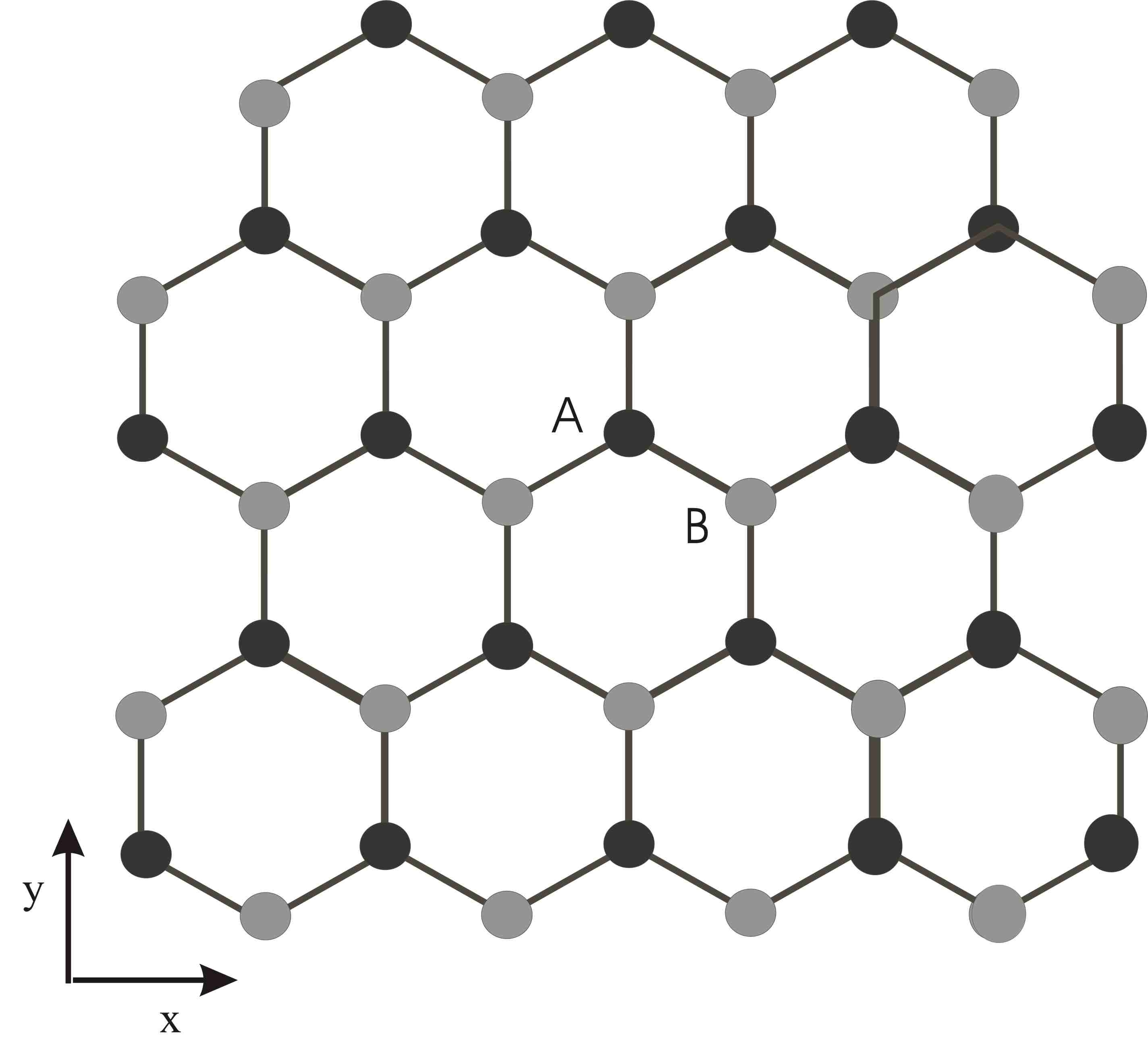
Figure 1: Spatial orientation of the monolayer graphene with respect to the $x$ and $y$ axis and A, B sublattices.

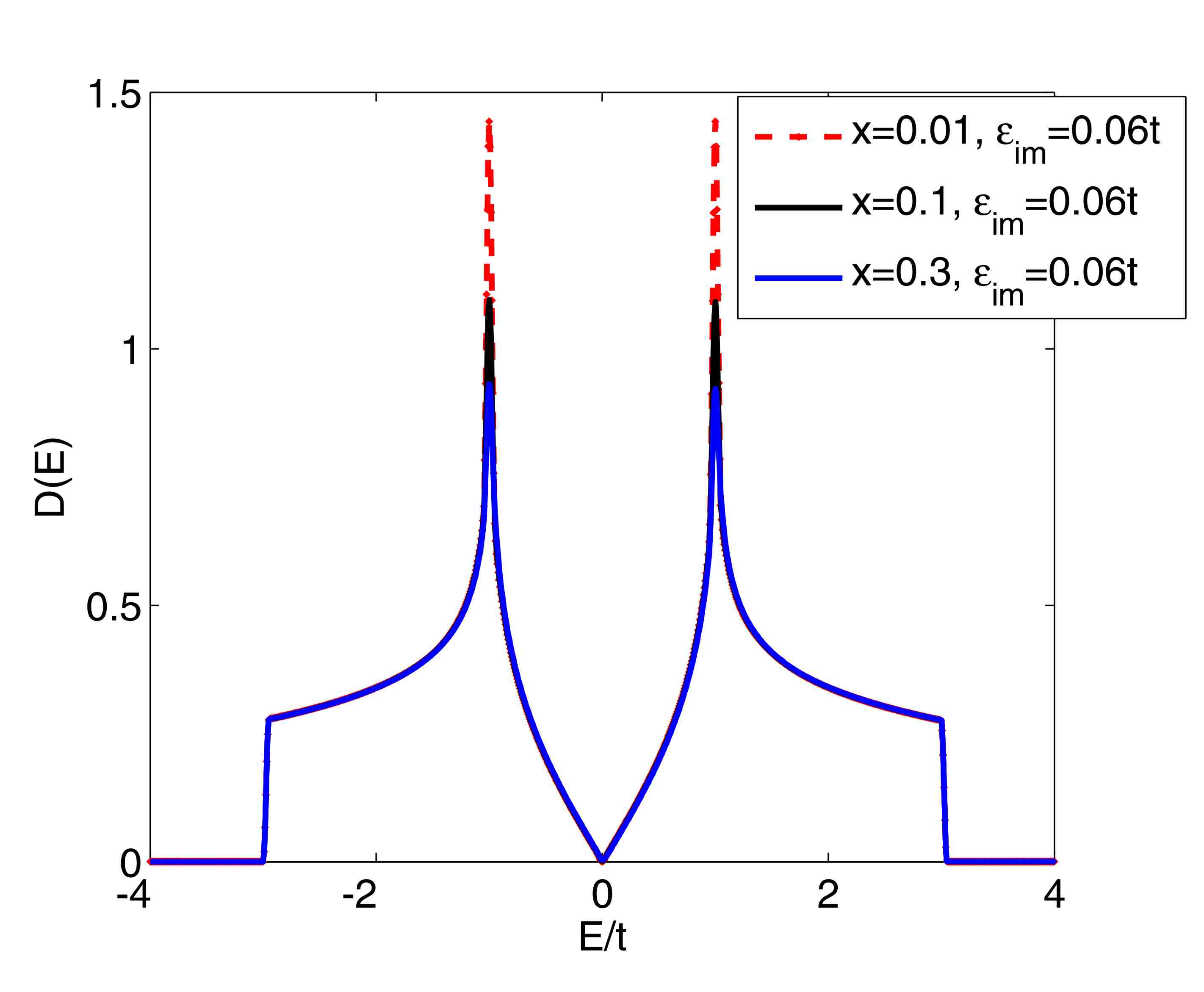
Figure 2: Density of states in graphene at different impurity densities and zero Rashba coupling.

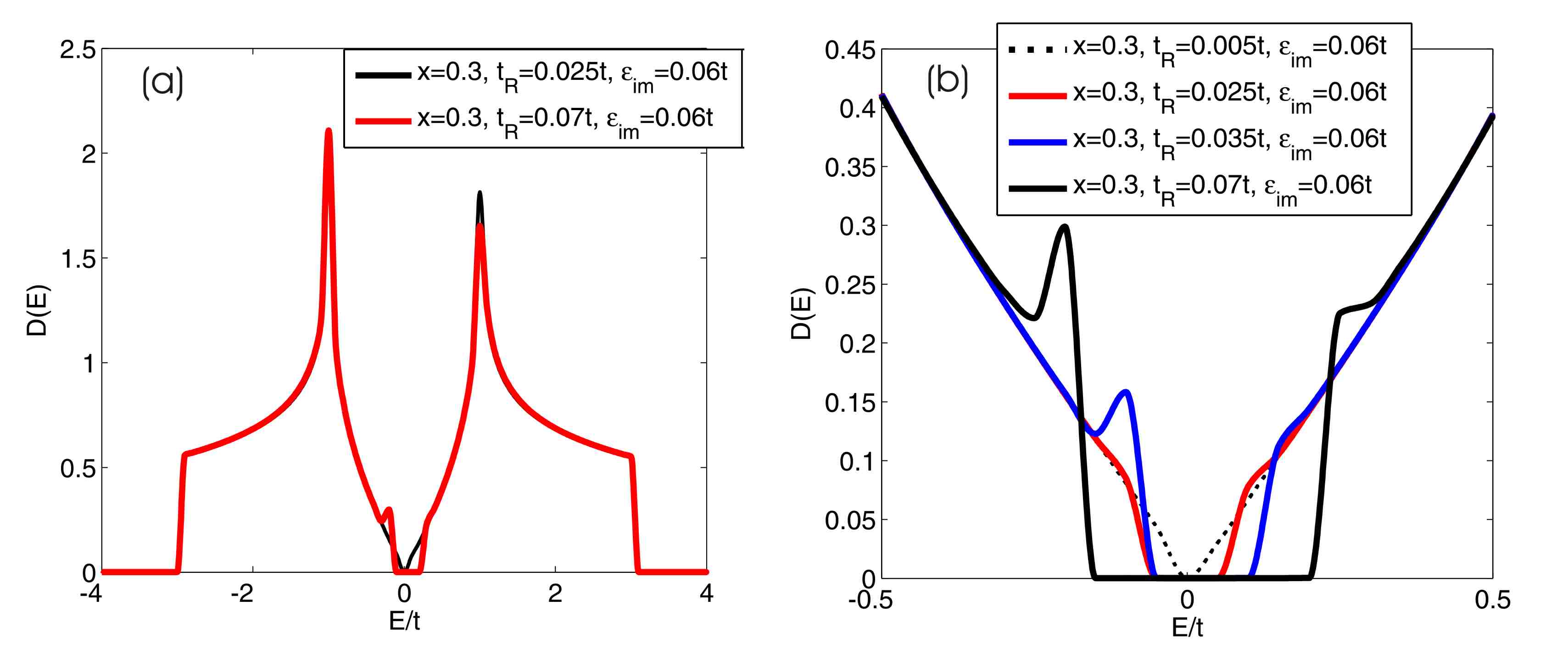
Figure 3: Density of states in graphene at different Rashba couplings. The symmetry of the conduction ($E>0$) and valence ($E<0$) bands has been broken by the Rashba interaction.

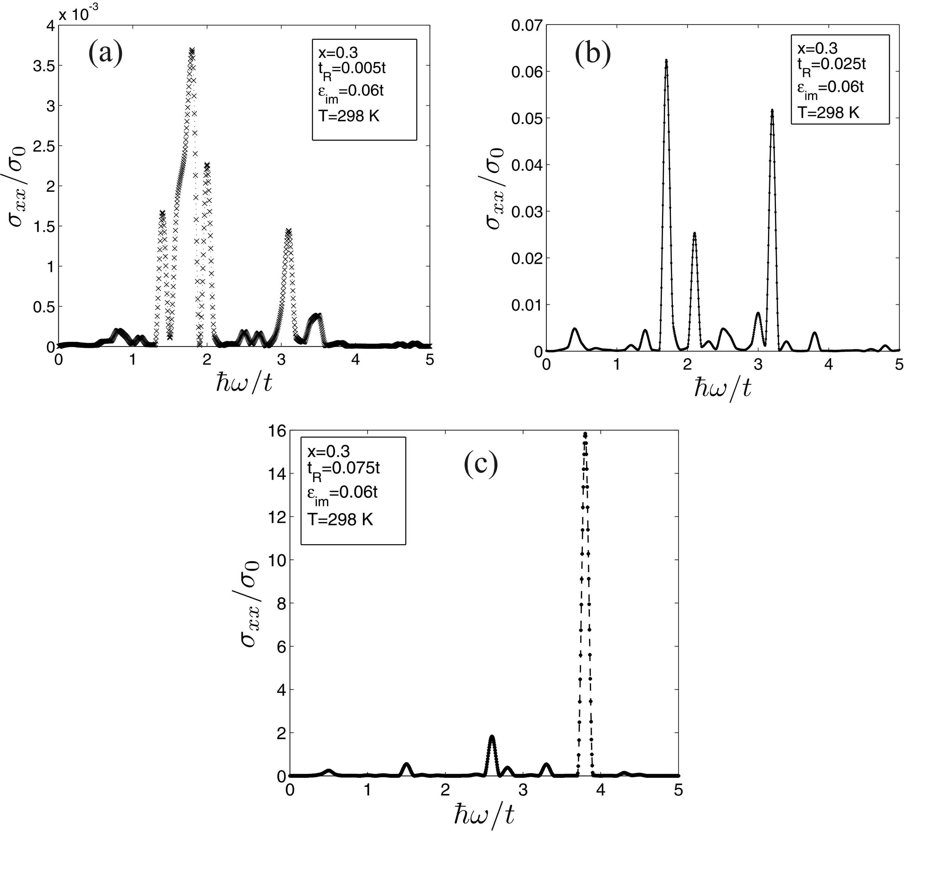
Figure 4: Optical conductivity along the x axis at different Rashba couplings (${{\sigma}_{0}}=\frac{{{e}^{2}}}{\hbar}$ ).

Figure 5: Anisotropic optical conductivity as a function of the photon energy at different Rashba couplings.

References

- [1] Y. Zhang, Y.-W. Tan, H. L. Stormer, P. Kim, Nature 438 (2005) 201.
- [2] A. Bostwick, T. Ohta, T. Seyller, K. Horn, E. Rotenberg, Nature Phys. 3 (2007) 36.
- [3] Antonio H. Castro Neto, Materialstoday, 13 (2010) 12.
- [4] S. Y. Zhou, G.-H. Gweon, A. V. Fedorov, P. N. First, W. A. de Heer, D.-H. Lee, F. Guinea, A. H. C. Neto, and A. Lanzara, Nature Materials 6 (2007) 770-775.
- [5] C.L. Kane and E.J. Mele, Phys. Rev. Lett. 95 (2005) 146802.
- [6] C.L. Kane and E.J. Mele, Phys. Rev. Lett. 95 (2005) 226801.
- [7] P. Rakyta, A. Kormányos, and J. Cserti,Phys. Rev. B82, 113405 (2010).
- [8] M. Gmitra, S. Konschuh, C. Ertler, C. Ambrosch-Draxl and J. Fabian, Phys. Rev. B 80 (2009) 235431.
- [9] D. Huertas-Hernando, F. Guinea, and A. Brataas,Phys. Rev. B 74 (2006) 155426.
- [10] J. C. Boettger and S. B. Trickey,Phys. Rev. B 75 (2007) 121402.
- [11] S. Konschuh, M. Gmitra, and J. Fabian,Phys. Rev. B 82 (2010) 245412.
- [12] S. Abdelouahed, A. Ernst, J. Henk, I. V. Maznichenko, and I. Mertig, Phys. Rev. B 82 (2010) 125424.
- [13] Yu. S. Dedkov, M. Fonin, U. Rudiger, and C. Laubschat,Phys. Rev. Lett. 100 (2008) 107602.
- [14] Ralph van Gelderen and C. Morais Smith Phys. Rev. B 81 (2010) 125435.
- [15] Z. Qiao, S. A. Yang, W. Feng, W.-K. Tse, J. Ding, Y. Yao, J. Wang, and Q. Niu,Phys. Rev. B82, 161414 (2010).
- [16] W. Wang, Ch. Zhang, Zh. Ma, J. Phys.: Condens. Matter 24 (2012) 035303.
- [17] T. Ando, T. Nakanishi, and R. Saito, J. Phys. Soc. Jpn. 67 (1998) 2857.
- [18] A. Phirouznia, S. Safari Shateri, J. PoursamadBonab, and K. Jamshidi-Ghaleh , Applied Physics Letters 101 (2012) 111905.
- [19] E. I. Rashba,Phys. Rev. B 79 (2009) 161409(R).
- [20] Johan Nilsson, A. H. Castro Neto, F. Guinea, and N. M. R. Peres, Phys. Rev. B 78 (2008) 045405.
- [21] R. Kubo, J. Phys. Soc. Jpn.12 (1957) 570.
- [22] E.N. Economou, ”Green Function In Quantum Physics” 3nd ed, Verlag Berlin Heidelberg, springer (2006).
Fig. 1