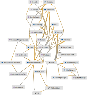
(a) Flat graph with 30 nodes and 65 links.

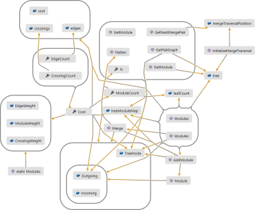
(b) Power Graph rendering computed using the heuristic of Royer et al. [12]: 7 modules, 36 links.

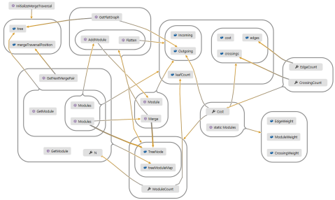
(c) Power Graph computed using Beam Search (see 4.1) finds 15 modules to reduce the link count to 25.

Improved Optimal and Approximate Power Graph Compression
for Clearer Visualisation of Dense Graphs

Abstract

Drawings of highly connected (dense) graphs can be very difficult to read. Power Graph Analysis offers an alternate way to draw a graph in which sets of nodes with common neighbours are shown grouped into modules. An edge connected to the module then implies a connection to each member of the module. Thus, the entire graph may be represented with much less clutter and without loss of detail. A recent experimental study has shown that such lossless compression of dense graphs makes it easier to follow paths. However, computing optimal power graphs is difficult. In this paper, we show that computing the optimal power-graph with only one module is NP-hard and therefore likely NP-hard in the general case. We give an ILP model for power graph computation and discuss why ILP and CP techniques are poorly suited to the problem. Instead, we are able to find optimal solutions much more quickly using a custom search method. We also show how to restrict this type of search to allow only limited back-tracking to provide a heuristic that has better speed and better results than previously known heuristics.

Introduction

In real-world applications such as biology and software engineering it is common to find network structures that are too dense to visualise in a way that individual links can still be followed. Such graphs occur frequently in nature as power-law or small-world networks. In practice, very dense graphs are often visualised in a way that focuses less on high-fidelity readability of edges and more on highlighting highly-connected nodes or clusters of nodes through techniques such as force-directed layout or abstraction determined by community detection [8]. Dense edge clutter may be alleviated to better show node labels by rendering the edges very faintly or with aggregate techniques like bundling [6]. Though such approaches may give a rough indication of the general graph structure they make following precise edge paths difficult or impossible.

Such path following is even more difficult when graphs are directed. Distinguishing direction on edges allows for up to twice as many distinct edges in the graph. For people trying to understand the graphs to accurately follow directed paths, edge curves must be drawn in enough isolation that any indications of direction (such as tapering, arrowheads or gradients [5]) are clearly visible.

Recently, alternative approaches have been suggested that attempt to retain the fidelity of individual edge paths by introducing drawing conventions that allow a large number of actual edges to be precisely implied by a small set of composite edges. In particular, so-called Power Graph Analysis constructs a hierarchy over nodes, such that nodes with similar neighbour sets are placed in the same group or module. An edge connected to the module then implies a connection to each member of the module. Power Graph Analysis utilises lossless compression since—by contrast with bundling or community-based clustering—no information is lost in the rendering. That is, the technique can be said to be information faithful [9] such that the full graph can be reconstructed by careful inspection of the drawing. Figure Improved Optimal and Approximate Power Graph Compression for Clearer Visualisation of Dense Graphs gives a small example of the application of Power Graph Analysis techniques to a small software dependency graph.

Power Graph Analysis has been shown to have practical application to visualising biological networks [12], detecting communities in social and biological networks [14] and more recently in software dependency diagrams [3]. A recent user study has shown that—for path-finding tasks—power-graph style groupings were more readable than flat graphs, even for people with very little training [3].

Relatively little attention has been devoted to algorithms for finding power graph decompositions, i.e. the best choice of modules in the power graph. Royer et al. [12] give a heuristic for finding the decomposition and Dwyer et al. [3] give a constraint programming formulation for finding the optimal decomposition with respect to various criteria, such as fewer edges or fewer edges crossing group boundaries. Unfortunately, an empirical evaluation of the two algorithms given in [3] reveals that the heuristic of  [12] is not very effective at finding an optimal solution while the constraint programming approach is too slow for practical use, taking days to run for larger graphs. Thus, we need better methods to find power graph decompositions. This is the subject of this paper. In particular, we focus on finding power-graphs that are optimal or approximately optimal with respect to the number of edges in the decomposition.

In Section 2 we prove that the problem of minimising the number of edges in a power graph decomposition with only one group is NP-hard. This is strong evidence that the general problem is NP-hard, though specific proofs for unrestricted modules and different goal criteria are needed.

In Section 3 we look at declarative models of the Power Graph problem for input into general-purpose solvers. In particular, we offer some refinements to the Constraint Programming model introduced in [3] (Section 3.1) and propose a new Integer Linear Programming model (Section 3.2).

In Section 4 we explore explicit search methods. In Section 4.1 we introduce a beam-search based approximate method that produces power graphs for a given flat graph, that are much closer to optimal than previous greedy heuristics. In Section 4.2 we extend this method to a full-backtracking search strategy that is able to find optimal power graphs relatively efficiently using a lower-bound calculation to cut branches of the search that are not useful. Our experiments (Section 5) show that this approach is orders of magnitude faster than solving the declarative models using generic solvers.

1 Background and Definitions

(d) A small graph with 23 edges.

(e) A power graph decomposition of the same graph can be drawn with only 7 edges.

Figure 1: A small example of power-graph decomposition.

Royer et al. [12] coined the term Power Graph Analysis to describe a technique for reducing edge clutter by introducing a module hierarchy over an undirected graph, such that edges connected to modules imply a connection to every child of the module. More formally, for a directed graph $G=(V,E)$ a power graph configuration is a set of modules $M$ where each module $m\in M$ is a subset of $V$. We assume that $M$ includes the set of trivial modules $\{\{v\}\mid v\in V\}$. Our use of the term module is due to the similarity with modules considered in Modular Decomposition. Like Modular Decomposition, modules can be nested to form a hierarchy and if two modules overlap one must be fully contained in the other. That is, for $m,n\in M$, if $m\bigcap n\neq\emptyset$ then $n\subset m$ or $m\subset n$. As in Modular Decomposition, a power graph decomposition is drawn with a set of representative edges $R$ uniquely specified by $E$ and $M$, such that a representative edge between two modules represents a complete bipartite graph in $E$ over the children of the two modules. That is, for two modules $m$ and $n$, a representative edge $(m,n)\in R$ represents the set of edges $\mathit{rep}(m,n)=\{(u,v)\mid u\in m,v\in n\}$. In drawings of power graphs, the set of representative edges $R$ must be minimal, i.e. $\nexists e_{1},e_{2}\in R$ s.t. $\mathit{rep}(e_{1})\subset\mathit{rep}(e_{2})$.

Unlike Modular Decomposition, however, the power graph definition above allows a representative edge to span module boundaries. For example, in Figure 1(e), the edge from node 5 to module $\{0,2,4\}$ implies that $E$ contains edges $(5,0),(5,2),(5,4)$ but says nothing about any modules containing node 5. This permits greater compression than modular decomposition, but can also cause confusion when reading the diagram, as considered by Dwyer et al. [3].

Royer et al. introduced a simple heuristic for obtaining the power graph decomposition for a given graph in $O(|V|^{3}|E|\log|E|)$ time. Their procedure involved first computing a “candidate module hierarchy” over the nodes in the graph by repeated greedy matching of nodes or modules with similar Jaccard index between their neighbour sets. A second iterative phase involves greedily instantiating the module that reduces the most edges. This is repeated until no more edge reduction is possible.

This algorithm is reasonably fast but—as we show in Section 5—produces results that are far from optimal. The Beam Search method described in Section 4.1 has faster run-time (depending on a beam size parameter) and finds solutions that are very close to optimal. Furthermore, in Section 4.2, we show that it is easy to introduce backtracking into this explicit search method, to produce a search that returns an optimal solution. Such a complete search is orders of magnitude faster than the best we have been able to achieve with generic solvers applied to declarative models, despite extensive experimentation with redundant constraints to limit the search space in those models, as described in Section 3.

2 Complexity Analysis

In this section we show that computing the optimal power-graph with a single module is NP-complete for undirected bipartite graphs. It then follows that the result holds for directed graphs in general. As an optimal module for a single module case need not be a module in the optimal power-graph with multiple modules (see Figure 2), it seems likely that it is hard in the general case too. Finding an optimal single module is equivalent to finding a biclique subgraph $(A,B)$ (here $A$ and $B$ denote the two independent sets of nodes) that maximises the edge savings, that is, $|A||B|-|A|$, $|A|\leq|B|$. The largest part, $B$, is taken to be the single module. This problem is different to the Maximum Vertex Biclique Problem (MVBP) that finds an induced biclique that maximises the number of nodes, $|A|+|B|$, and to the Maximum Edge Biclique Problem (MBP) that finds a biclique subgraph that maximises the number of edges, $|A||B|$. For example, a biclique with $|A_{1}|=3$ and $|B_{1}|=4$ has more edges than a biclique with $|A_{2}|=1$ and $|B_{2}|=11$, but $B_{2}$ gives the maximum edge savings. Similarly, a biclique with $|A_{1}|=1$ and $|B_{1}|=9$ has more nodes than a biclique with $|A_{2}|=3$ and $|B_{2}|=6$, but $B_{2}$ give the maximum edge savings. Although MVBP can be solved in polynomial time for bipartite graphs [4, Comments on GT24][16], it is NP-complete for general graphs [15]. MBP was shown to be NP-Complete in [11] using a reduction based on the reduction used to show the NP-completeness of the Balanced Complete Bipartite Subgraph problem in [7]. We use this reduction to show that finding the optimal single module is NP-complete.

Figure 2: The optimal solution for a single module (shaded) is not in the optimal solution for two modules (dashed lines).

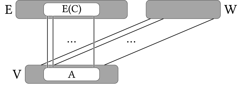
Figure 3: The construction $G^{\prime}$.

We define the problem MSMP (Maximum Single Module Problem) as follows: Given a bipartite graph $G=(V_{1},V_{2},E)$ and $k\in\mathbb{N}$, does $G$ contain a module that achieves an edge saving $\geq k$.

Theorem 2.1

MSMP is NP-complete.

Proof 2.2.

It is clear that MSMP is in NP. We reduce from CLIQUE [4] to MSMP using the transformation given in [11]. Let $G=(V,E)$ and $k\in\mathbb{N}$ be an instance of CLIQUE. Without loss of generality we assume $k=|V|/2\geq 5$. We construct a bipartite graph $G^{\prime}=(V_{1},V_{2},E^{\prime})$ (see Figure 3) such that $G^{\prime}$ contains a module with edge savings $\geq k^{3}-k^{2}-k$ if and only if $G$ contains a clique of size $k$. Let $V_{1}=V$ and $V_{2}=E\cup W$ where $W$ is a set of $\binom{k}{2}$ new nodes and $E^{\prime}=\{\{v,e\}:v\in V,e\in E\text{ and }v\text{ not incident to }e\}\cup\{\{v,w\}:v\in V,w\in W\}$. It is clear that this construction can be performed in polynomial time.

If $G$ contains a clique $C$ of size $k$ then $(A,B)$ where $A=V-C$ and $B=W\cup E(C)$ is a biclique subgraph of $G^{\prime}$. For $k\geq 5$, $|B|=2\binom{k}{2}\geq|A|=k$. Selecting $B$ as a module gives an edge savings of $|A||B|-|A|=k^{3}-k^{2}-k$.

Suppose $G$ has no clique of size $\geq k$. We show that any module in $G^{\prime}$ gives a saving of $<k^{\prime}=k^{3}-k^{2}-k$. Let $(A,B)$ be a maximal biclique in $G^{\prime}$, $A\subseteq V_{1}$ and $B\subseteq V_{2}$. We note that any maximal biclique has $W\subseteq B$ and as $|A|\leq|V|=2k\leq|W|\leq|B|$ when $k\geq 5$, $B$ would be the optimal module.

Now $B=W\cup B^{\prime}$ where $B^{\prime}$ corresponds with the edges in $G$ whose endpoints are not in $A$. So $|B^{\prime}|\leq(|V|-|A|)(|V|-|A|-1)/2=(2k-|A|)(2k-|A|-1)/2$.

There are two cases.

Case 1 $|A|>k$:

Suppose $|A|=k+c$, $c\in(0,k]$. Then

$$|A||B|-|A| \leq(k+c)\left(\frac{k(k-1)}{2}+\frac{(k-c)(k-c-1)}{2}\right)-(k+c)$$

$$=k^{3}-k^{2}-k-\frac{k}{2}\left(c^{2}+c\right)+\frac{c}{2}\left(c^{2}+c-2\right)$$

$$<k^{3}-k^{2}-k.$$

Case 2 $|A|\leq k$:

Suppose $|A|=k-c$, $c\in[0,k]$. Now as $G$ has no clique of size $\geq k$, the number of edges in the subgraph of $G$ induced by $V-A$ (and hence $|B^{\prime}|$) is $\leq\frac{(k-2)(k+c)^{2}}{2(k-1)}$ by Turán’s theorem [13]. So

$$|A||B|-|A|\leq (k-c)\left(\frac{k(k-1)}{2}+\frac{(k-2)(k+c)^{2}}{2(k-1)}\right)-(k-c)$$

$$\leq k^{3}-k^{2}-k$$

$$-\frac{1}{2(k-1)}\left((c^{2}+1)k^{2}-2c^{2}k+c(c^{2}-1)(k-2)\right)$$

$$< k^{3}-k^{2}-k$$

for $k\geq 5$. $\Box$

3 Declarative Models

In this section we investigate how two standard generic methods for solving combinatorial optimisation problems, constraint programming and integer liner programming (ILP), can be applied to solve the optimal power graph decomposition problem. The advantage of using such generic approaches is that they allow the model to be relatively easily specified in a declarative language such as MiniZinc  and then run with powerful state-of-the-art solvers.

3.1 Constraint Programming

Our starting point is the constraint programming formulation for finding the optimal power graph decomposition given in [3]. The input to the model is the number of vertices $nv$, a Boolean array $\mathit{edge}$ which is the adjacency matrix for the edges in the original graph, a limit on the number of modules $ml$ and an upper bound $ub$ on the objective function. To solve the complete problem we can set $ml=nv$ and $ub=\infty$.

The main decision variables in the problem are the number of modules $\mathit{anm}$ and the Boolean array $\mathit{module[v,m]}$ which gives the vertices $v$ in each module $m$, i.e. $\mathit{module}[v,m]\leftrightarrow v\in m$. There are 3 kinds of modules. Modules $1...nv$ are trivial. We constrain these to have a single vertex in them, i.e. module $v$ is the trivial module $\{v\}$. Modules $nv+1...anm$ are real modules while modules $anm+1..nm$ are dummy modules where $nm=nv+ml$. The dummy modules are constrained to be empty.

We require that the modules form a hierarchy: this is enforced by requiring for all modules $m$ and $n$, $m\subseteq n\vee n\subseteq m\vee m\cap n=\emptyset$. The formulation makes use of Boolean array $\mathit{mcontains}[m,n]$ which is constrained to hold if module $m$ contains module $n$.

Our objective function is to minimise the number of edges in the power graph. For any fixed choice of modules there is a unique best choice of edges in the power graph. We compute for each pair of nodes $m$ and $n$ if there is a possible edge between them. There is a possible edge between $m$ and $n$ iff: (1) for all $u\in m$ and for all $v\in n$, $(u,v)\in E$, and (2) $m=n$ or $m\cap n=\emptyset$. From this we can compute the actual edges in the power graph. This is any possible edge $(m,n)$ which is not dominated by some other possible edge $(m^{\prime},n^{\prime})$ where $(m^{\prime},n^{\prime})$ dominates $(m,n)$ if $m\subseteq m^{\prime}$ and $n\subseteq n^{\prime}$.

We extended the model from [3] with a number of redundant and symmetry breaking constraints that significantly improved its efficiency.

1. To stop arbitrary re-ordering of the modules we added the symmetry breaking constraint that the real and dummy modules were in decreasing lexicographic order using the standard global function $\mathit{lex\_greatereq}$.

2. We added the redundant constraint that if two vertices have the same ingoing and outgoing edges then they should be in exactly the same set of modules: clearly this is true in an optimal solution.

3. We added a redundant formulation of module containment based on the observation that the scalar product $sp[m,n]$ of two modules $m$ and $n$ is $|m|$ iff $m\subseteq n$.

4. We added a redundant constraint that every module must have at least one potential edge from it: i.e. there is at least one node that has an edge to all of the nodes in the module.

3.2 Integer Linear Programming (ILP)

In our next approach we explored the use of ILP. Mathematical programming techniques like ILP can often outperform constraint programming on particular problems. A disadvantage, when compared to constraint programming, is it can be difficult to formulate a given problem as a mathematical program. Here we formulate an integer linear program that minimizes the number of edges. A more detailed description of the model can be found in the Appendix.
Input and Parameters

$n$ is the number of vertices of the input graph $G$.
$V=\{0,1,\dots,n-1\}$ represents the vertices of the input graph $G$.
$e(u,v)$ represents the edges of the input graph $G$ as an incidence matrix. That is, $e(u,v)=1$ if $(u,v)$ is an edge of $G$ and $e(u,v)=0$ otherwise.
$m$ is the number of modules with at least two elements (we consider each singleton vertex to belong to its own module).
$M=\{0,1,\dots,n+m-1\}$ represents the set of all modules.

Integer decision variables

$sav[m_{1},m_{2}]$ the number of edges that may be removed from $G$ (to then be replaced by a single edge) if the modules $m_{1}$ and $m_{2}$ are added.

Binary decision variables

$mod[v,m]$ takes the value $1$ if and only if vertex $v$ belongs to the module $m$.
$ind[v,m]$ takes the value $1$ if and only if $(v,u)$ is an edge, for all $u$ in the module $m$.
$bic[m_{1},m_{2}]$ takes the value $1$ if and only if, for every vertex $v\in m_{1}$ and every vertex $u\in m_{2}$, the pair $(u,v)$ is an edge in $G$.
$dis[m_{1},m_{2}]$ takes the value $1$ if and only if the modules $m_{1}$ and $m_{2}$ are disjoint sets of vertices.
$sub[m_{1},m_{2}]$ takes the value $1$ if and only if the module $m_{1}$ is a proper subset of the module $m_{2}$.
$mInd[v,m_{1},m_{2}]$ takes value $1$ if and only if $v\in m_{1}$ and $ind[v,m_{2}]=1$.
$vMod[v,m_{1},m_{2}]$ takes value $1$ if and only if $v\in m_{1}$ and $v\in m_{2}$.
$sVer[v_{1},v_{2},m_{1},m_{2}]$ takes value $1$ if and only if $(v_{1},v_{2})$ is an edge with $v_{1}\in m_{1}$ and $v_{2}\in m_{2}$ and the edge $(v_{1},v_{2})$ can be removed if $m_{1}$ and $m_{2}$ are added.
$sMod[m_{1},m_{2}]$ takes value $1$ if and only if $sav[m_{1},m_{2}]>0$.

Objective

Maximise

$$\sum\{sav[m_{1},m_{2}]-sMod[m_{1},m_{2}]\mid m1,m2\in M,\ m_{1}\neq m_{2}\}.$$

Constraints

The majority of the constraints in our ILP model are purely to correctly define binary decision variables and so we have omitted them for brevity.

1. $dis[m_{1},m_{2}]+sub[m_{1},m_{2}]+sub[m_{2},m_{1}]=1$, $m_{1}\neq m_{2}\in M$.

2. $\sum\{sVer[v_{1},v_{2},m_{1},m_{2}]\mid m_{1},m_{2}\in M,m_{1}\neq m_{2}\}\leq 1$, $v_{1},v_{2}\in~{}V$.

3. $sav[m_{1},m_{2}]\leq\sum\{sVer[v_{1},v_{2},m_{1},m_{2}]\mid v_{1},v_{2}\in V,v_{1}\neq v_{2}\}$, $m_{1}\neq m_{2}\in M$.

4. $sMod[m_{1},m_{2}]\leq sav[m_{1},m_{2}]$, $m_{1}\neq m_{2}\in M$.

5. $sav[m_{1},m_{2}]\leq n^{2}sMod[m_{1},m_{2}]$, $m_{1}\neq m_{2}\in M$.

6. $\sum\limits_{v\in V}mod[v,m_{1}]=1$, $m_{1}\in V$.

7. $mod[m_{1},m_{1}]=1$, $m_{1}\in V$.

Constraint 1 states that for any two distinct modules $m_{1}$ and $m_{2}$, either $m_{1}$ and $m_{2}$ are disjoint, or one is a proper subset of the other. Constraint 2 says that no edge can be counted twice in the saving calculation. Constraint 3 defines the variables $sav[m_{1},m_{2}]$. Constraints 4 and 5 defines $sMod[m_{1},m_{2}]$. Constraints 6 and 7 force each vertex to be a singleton module.

4 Explicit Search Methods

Figure 4: The search space of module configurations for a given graph is a tree structure. Here we highlight several nodes in the very large search space of module configurations for the graph shown in Figure 1. A solid arrow indicates a direct child relationship in the search tree. That is, the child configuration is obtained from a single merge operation from the parent. A dotted arrow indicates the target configuration is reachable from the source via multiple merges.

As defined in Section 1, for a given flat graph, a configuration is a set of modules, where each module is a set of vertices of the graph and other modules such that the modules form a hierarchy. The objective is to find a configuration that minimises the number of edges.

A configuration can be constructed by adding one module at a time. The order in which the modules are added has no effect, so we impose a constraint that only top-level modules are added – that is, if the configuration is $\{m_{1},m_{2},\dots,m_{n}\}$, then a new module must not be a subset of any $m_{i}$.

The set of possible module configurations is then a tree, with the configuration containing only trivial modules (the flat graph) at the root, as illustrated in Figure 4. Each node in the tree has one child for each module that can be added to that configuration.

To prevent multiple paths to the same configuration, we impose an arbitrary ordering on the children of a node, and force that if $m_{1}$ and $m_{2}$ are two sibling child modules such that $m_{1}$ appears to the left of $m_{2}$, then the module $m_{1}$ may not appear in any configuration in the subtree of $m_{2}$.

Thus, this tree will contain every possible configuration of modules, and a search for the best configuration may simply do a full traversal of the tree; however, this is impractically slow. In the remainder of this section we describe how to improve the efficiency of this search.

4.1 Beam Search

Using the above definitions, we can define greedy heuristics to obtain a power-graph configuration with significantly fewer representative edges than are required to draw the flat graph.

To limit the branching at each search-tree node $t$ associated with a configuration $C$, we restrict children of $t$ to be those obtainable through a merge of two top-level modules in $C$. That is, a merge of modules $m$ and $n$ creates a new configuration $C^{\prime}=C\cup\{\{v\}\mid v\in m\cup n\}$.

A simple best-first search is—for a given starting configuration $C$ with $n_{t}$ top-level modules—to try all possible merges to give $\{C^{\prime}_{1},\ldots,C^{\prime}_{n_{t}(n_{t}-1)}\}$ children and then simply take the one with the fewest representative edges to be the next configuration. We repeat until no further improvement is possible.

Since the set of representative edges $R$ used to draw the power graph must be minimal, such a merge operation may leave $m$ or $n$ with no associated representative edges, i.e. $\mathit{rep}(m,\_)=\emptyset$ or $\mathit{rep}(\_,n)=\emptyset$. Since a module with no associated edge in $R$ serves no purpose, we remove such modules from the merge result $C^{\prime}$.

In practice, a full merge is not required just to calculate the reduction in edges achieved by the merge. Consider a merge of two modules $m$ and $n$ in $C$ with representative edges $R(C)$ giving a configuration $C^{\prime}$ with edges $R(C^{\prime})$. If the outgoing and incoming neighbour sets in $R$ of $m$ are given by $N^{+}(m)$ and $N^{-}(m)$, then the number of edges in $R(C^{\prime})$ will be precisely:

$$\mathit{nedges}(m,n)=|R(C)|-|N^{+}(m)\cap N^{+}(n)|-|N^{-}(m)\cap N^{-}(n)|$$

Applied to a graph $G=(V,E)$, $O(|V|)$ such greedy merges are possible before no more improvement is possible. Since a given module may include all edges in its neighbour set, computing $\mathit{nedges}(m,n)$ can be $O(|E|\log|E|)$ and to find the best possible merge this must be computed for all pairs of modules. Therefore, a naïve implementation could take $O(|V|^{3}|E|\log|E|)$ time though in practice the number of modules that must be considered and the size of their neighbour sets diminishes quickly.

Beam search [10, p. 195] gives us a way to introduce some limited backtracking into this best-first strategy. Instead of only considering the single best merge at each iteration, we maintain a beam of the $k$ best solutions found so far. The full process is shown in Algorithm 1.

One detail in this algorithm is the check before insert of a configuration into the beam that we have not already considered a configuration that is structurally identical. This is done by maintaining a hashset $S$ with signatures of configurations previously inserted into the beam. For a configuration $C$ the signature $\mathrm{sig}(C)$ is obtained by a canonical (ordered) traversal of the module hierarchy.

Data: A starting configuration of modules $C_{0}$ with representative edges $R_{0}$. A beam size $k\geq 1$.

Result: An improved configuration $C^{\star}$ with $|R^{\star}|\leq|R_{0}|$

$\mathsf{beam}\leftarrow$ priority queue of configurations

such that first element in queue has maximum $|R|$;

push$(\mathsf{beam},C_{0})$;

$S\leftarrow$ hashset of signatures of configurations in $\mathsf{beam}$;

repeat

       $(\mathsf{improved},\mathsf{currentbeam})\leftarrow$ (false, copy $\mathsf{beam}$);

       foreach $C\in\mathsf{currentbeam}$ do

             $\mathsf{merges}\leftarrow\{(e,m,n)\mid$

             $e\leftarrow\mathit{nedges}(m,n),(m,n)\in C\times C\}$;

             $\mathsf{kbest}\leftarrow$ from $\mathsf{merges}$ take $k$ triples $(e,m,n)$

             with smallest $e$ where $sig(C,(m,n))\not\in S$;

             foreach $(e,m,n)\in\mathsf{kbest}$ do

                   $b\leftarrow$ first (i.e. worst) configuration in $\mathsf{beam}$;

                   if $|\mathsf{beam}|<k$ or $|R(b)|>e$ then

                         $C^{\prime}\leftarrow\mathrm{merge}(m,n)$;

                         push$(\mathsf{beam},C^{\prime})$;

                         insert$(S,\mathrm{sig}(C^{\prime}))$;

                         $\mathsf{improved}\leftarrow$ true;

                        

                   end if

                  if $|\mathsf{beam}|>k$ then

                         pop$(\mathsf{beam})$;

                        

                   end if

                  

             end foreach

            

       end foreach

      

until not $\mathsf{improved}$;

return configuration in beam with smallest $|R|$

Algorithm 1 Beam Search

4.2 Optimal Search

We can show certain properties of the configuration tree that will help us to eliminate regions of the tree without missing any optimal configurations. First, we restrict the definition of “optimal” to be a configuration that has no redundant modules. That is, if two configurations $C$ and $C\cup\{m\}$ have the same objective cost, only $C$ can be considered optimal.

Adding a module cannot increase the number of edges. Any new edge added to the graph must replace some existing edges. A new edge between existing module $m$ and new module $n$ replaces all previous edges between members of $m$ and members of $n$. Since there must be at least one such previous edge, the number of edges removed is at least the number of edges added.

Every optimal configuration can be reached by a sequence of improving module additions. That is, every module added reduces the number of edges.

An outline of the reasoning is as follows. Let the desired optimal configuration be $C=\{m_{1},m_{2},\dots,m_{n}\}$. Starting from the empty configuration, choose any module that contains no sub-modules. Adding this module will reduce the number of edges, so add it to the current configuration. This module must reduce the number of edges – if it didn’t, then $C$ wouldn’t be optimal. Then after adding this module, find another module that contains no sub-modules (or only sub-modules that have already been added) and add that module, and so on.

An optimal solution has at most $n-2$ modules, where $n$ is the number of vertices in the flat graph. A configuration can have at most $n-1$ modules. A configuration with $n-1$ modules must include a module that contains all vertices in the graph. However, such a module is not an improving module and so cannot appear in an optimal solution. Therefore, an optimal configuration can have at most $n-2$ modules.

If adding module $m$ to configuration $C$ would remove $e$ edges, then adding module $m$ to configuration $C^{\prime}\supset C$ would remove at most $e$ edges.

Adding a module $m$ with members $\{a,b,\dots\}$ to configuration $C$ can only remove edges by replacing existing edges $\{(a,v),(b,v),\dots\}$ with a single edge $(m,v)$ (and similar for opposite-oriented edges). A configuration $C^{\prime}\supset C$ has the same set of edges as $C$, except that some edges are replaced by a smaller set of edges. Therefore, the module $m$ can only replace the same set of edges $\{(a,v),(b,v),\dots\}$ or a smaller set where some of those edges have been merged.

These properties allow us to calculate a lower bound on the best possible configuration in under a given configuration in the search tree. Given a configuration $C$ with $m$ modules, we can compute the minimum number of edges for any configuration that is a superset of $C$.

Let $c_{1},c_{2},\dots,c_{n}$ be the modules permitted to be added to configuration $C$. Each of these can be given a score $S(c_{i})$ that is the number of edges removed by adding that module: $S(c_{i})=E(C)-E(C\cup\{c_{i}\})$. Since we can add at most $n-2-m$ modules to $C$, the most edges we can possibly remove from $C$ is the sum of the best $n-2-m$ scores of the modules $c_{1},c_{2},\dots,c_{n}$.

Therefore, for a given configuration $C$ we can calculate the score of a hypothetical configuration $C^{\prime}\supset C$ that has the minimum possible edges. (The configuration is only hypothetical because it likely violates the hierarchy restriction on the modules.) If the objective cost of $C^{\prime}$ is no better than the best-known solution, the search can backtrack immediately from $C$. An outline of the exhaustive search algorithm is given in Algorithm 2.

Data: Current configuration, incumbent configuration, flat graph.

Result: The optimal configuration.

if current configuration is better than incumbent then

       record current configuration as incumbent

end if

$\mathsf{bound}\leftarrow$ compute bound of current configuration;

if $\mathsf{bound}$ is not better than incumbent then

       backtrack;

      

end if

if current configuration below module limit then

       $\mathsf{modules}\leftarrow$ modules that can be added to current configuration;

       Sort $\mathsf{modules}$ with most edge-reducing modules first;

       for each module $m\in\mathsf{modules}$ do

             Recurse with $m$ added to current configuration;

             Upon backtracking, forbid $m$ from $\mathsf{modules}$;

            

       end for

      

end if

return incumbent configuration

Algorithm 2 Outline of optimal search.

We can further reduce the number of modules considered at each step of the search. We only need to consider binary modules—as produced by the merge operation for the beam search (Section 4.1)— which have exactly two members (which themselves may be either modules or single vertices). The search is still guaranteed to find an optimal configuration.

Any optimal configuration has a counterpart that has only binary modules, and each such binary module reduces the number of edges. Consider an optimal configuration $C$, constructed by the sequence of modules $<m_{1},m_{2},\dots,m_{n}>$. Let $m_{i}$ be a non-binary module. We can convert $m_{i}$ into a binary module by grouping together two of its members arbitrarily. (This newly created sub-module will have no edges: if it was beneficial for this new sub-module to have edges, $C$ would not have been optimal.) The new sub-module is inserted immediately before $m_{i}$ in the construction sequence. If $m_{i}$ is still not binary, recurse.

All new sub-modules created in this way reduce the number of edges during construction. We know that adding the non-binary module $m_{i}$ reduces the number of edges. From this we know that the members of $m_{i}$ share at least one common predecessor or common successor. Therefore, any pair of the members of $m_{i}$ share a common predecessor or successor, and adding a module containing just that pair will reduce the number of edges. (Any modules that become redundant during this construction can be removed.)

The consequence of this property is that in the search algorithm, the modules to be added at each step need only be these binary modules instead of all possible modules. This greatly reduces the search space.

5 Experiments

5.1 Heuristic Methods

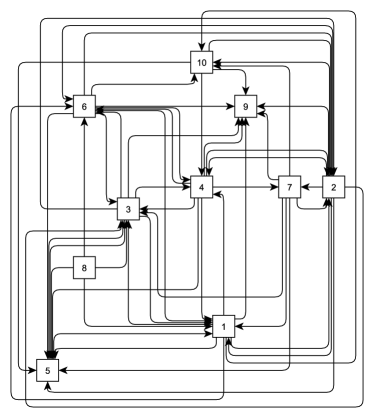
(a) Flat graph with $|V|=10,|E|=51$. An orthogonal layout style was used (Y-Files implementation of topology-shape metrics approach) in an attempt obtain a layout and routing in which each individual edge path is traceable. Such traceability is necessary to support discerning reachability or path-finding tasks.

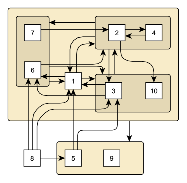
(b) Greedy Jaccard Metric decomposition. Decomposition has 5 modules, 23 edges and 21 crossings between edges and module boundaries.

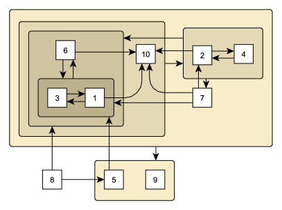
(c) Beamsearch decomposition $k=1$. Decomposition has 6 modules, 19 edges and 17 crossings between edges and module boundaries.

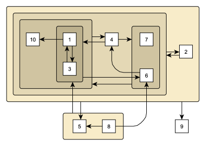
(d) Optimal decomposition obtained with beam search $k=10$ (optimality proven with method described in Section 4.2). Decomposition has 6 modules, 16 edges and 13 crossings between edges and module boundaries.

Figure 5: Flat and power graph renderings of a graph with 10 nodes and 51 edges. It is interesting to note that the reduction in clutter from 5(b) to 5(c) is fairly obvious, however, the qualitative improvement from 5(c) to 5(d) is less dramatic. Layouts were obtained using the yEd software (%****␣experiments.tex␣Line␣25␣****http://yfiles.com) using a combination of automatic layout and manual refinement with automatic edge routing.

Following Dwyer et al. [3], we generate random scale-free directed graphs with various numbers of nodes using the model of Bollobás et al. [1]. To generate a graph with $|V|$ nodes we control for density such that the number of edges is roughly proportional to $\frac{3}{2}|V|^{\frac{3}{2}}$. For example, a graph with 10 nodes will have around 50 edges, while a graph with $|V|=100$ will have around 1500 edges.

All heuristics were implemented in $C\#$ and run on a modern tablet PC. The source-code is available under an open-source license.

Figure 6 compares the decompositions obtained by applying our various heuristic powergraph decomposition methods to graphs generated as described above. It is clear that the Greedy Jaccard Clustering method [12] (JC) is easily beaten in terms of quality of the final solution, even by beam search with a beam size $k$ of 1 (i.e. best-first search with no backtracking at all). Increasing $k$ to 10 does improve the results slightly even—in some cases—returning the optimal (e.g. see Figure 5(d)). However, this is achieved at a ten-fold increase in running time (see Figure 7). Increasing $k$ further to 100 only occasionally results in a slightly better solution. Note that with $k$ small compared to the total number of configurations in the search space there is no guarantee that beam search will return the optimal.

Figures 5(b), 5(c) and 5(d) show the renderings of the results obtained for a small instance with 10 nodes and 51 edges. The quality of the renderings in terms of visual clutter, does seem to reflect the numbers seen in Figure 6. There is a fairly marked visual improvement between JC (Figure 5(b)) and Beam Search with k=1 ($BS_{1}$) (Figure 5(c)), in particular $BS_{1}$ can be rendered without edge-edge intersections while for the JC decomposition it is impossible. However, there is a much less obvious improvement from $BS_{1}$ to $BS_{10}$ (Figure 5(d)): the latter has three fewer edges and four fewer edge-module boundary crossings. The result found by $BS_{10}$ is, in fact, the optimal as confirmed by running a full search.

In terms of running time, Beam Search with $k=1$ is easily the fastest method, as seen in Figure 7. Generally, the running time (and also memory requirements) for beam search grow linearly in $k$. For example, $BS_{10}$ has very close to twice the run time of $BS_{5}$. The exception is that the running time of $BS_{1}$ is significantly less than $10\%$ that of $BS_{10}$ since we are able to apply all the merges entirely in place and no copying of configurations is required nor checks for structural equivalence of configurations.

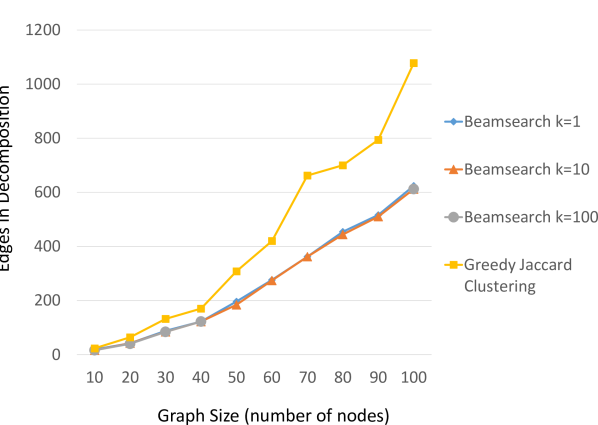
Figure 6: Comparison of cost versus graph size for the various power graph decomposition heuristics.

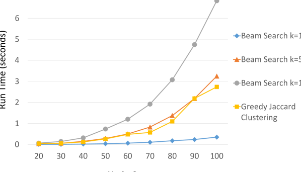
Figure 7: Comparison of running times for Beam Search with various beam sizes and Greedy Jaccard Clustering heuristic.

5.2 Optimal Methods

We have compared the efficiency of the exhaustive search methods across a corpus of 10-vertex graphs. The running times on a single representative graph are given below.

ILP model	$>160$ CPU hours
CP model without redundant constraints	$>72$ hours
CP model with redundant constraints	$26.6$ hours
Optimal Search	$8$ minutes
Optimal Search (edge-minimization only)	$22$ seconds

Note that the ILP model only tries to minimize edges, while both variants of the CP model try to break ties by minimising the number of module boundary crossings and number of modules as in [3]. For comparison with the CP model, we implemented two variants of the optimal search: one only minimising edges, and the other breaking ties in the same way as the CP model. The tie-breaking variant is slower because it explores a larger search space and must do more work at each search step to compute boundary crossings.

All exhaustive methods were run on an Intel Core i7 2.67 GHz CPU. The ILP solver was run in parallel, with 8 cores running for 20 hours. The ILP model was run with the commercial Gurobi solver, and the CP model was run with the lazy-clause generation solver CPX. The ILP model and CP model without redundant constraints failed to find the optimal solution. The other three methods found the optimal solution and proved it to be optimal.

6 Conclusion

This paper has presented a number of results, both practical and theoretical. On the practical side, the best-first search method (or beam search $k=1$ or $BS_{1}$) is much faster than the previous best available heuristic, the Greedy Jaccard Clustering [12] (JC). For example, a dense graph with 100 nodes and 1500 edges can be decomposed in 0.35 seconds with $BS_{1}$ compared to 2.74 seconds for JC. This is a significant enough performance improvement to enable new scenarios like continuous decomposition of live-streaming dynamic graph data.

Our experiments have shown that it also computes decompositions that are much closer to optimal, e.g. for the graph above $BS_{1}$ achieves a decomposition with 624 edges compared to 1078 for JC. We have also shown the applicability of the beam search technique to obtain still more optimal results (e.g. again for the 100 node graph $BS_{10}$ finds a 612 edge decomposition) in reasonable time and memory.

For the optimal power graph decomposition problem, we have contributed the first known ILP model and significant improvements to a previous CP model. While there have been many improvements to the compiler and solver technologies for such mathematical programming techniques this problem still defies simple, efficient declarative models. By contrast, we have provided an explicit search method that is able to find and prove optimality in minutes compared to days. Truly optimal solutions may not be necessary for practical power graph visualisation, but being able to efficiently compute them at least for small instances has proven invaluable in helping us develop better heuristic methods such as the beam search. For example, development of the beam search was in large part motivated by discovering just how bad the Jaccard clustering method was by comparison to optimal decompositions.

On the theoretical side we give the first known NP-hardness proof for a power-graph analysis problem (the one module case) which is strong ground-work for a general NP-hardness proof, though it is also likely that variations of the problem (such as slightly different constraints or goal functions) may require separate proofs or may even be polynomial time.

7 Further work

As mentioned above more complexity analysis is required for the general power graph problem and its variants.

A related technique for simplifying dense graphs is confluent graph drawing [2]. Like power-graph decomposition this also involves identifying bipartite components. Current confluent graph drawing algorithms have tended to focus on the computability of planar confluent graphs. There has been little focus on developing methods that can do something reasonable when a planar drawing is not possible. We think an optimisation-based approach related to the techniques described in this paper may have some success in this regard.

Finally, we need better layout methods for power-graph decompositions and clustered graphs generally. The examples in this paper were initially arranged with the Y-Files organic layout method but required significant manipulation to achieve pleasing alignment and to minimise crossings between edges.

Appendix

For the published version of this paper these additional details will be provided as an on-line tech report.

Appendix A ILP model

The following is a complete description of the ILP model used to minimise the number of power edges (or equivalently to maximise the number of edges saved by adding modules). Input and Parameters

$n$ is the number of vertices of the input graph $G$.
$V=\{0,1,\dots,n-1\}$ represents the vertices of the input graph $G$.
$e(u,v)$ represents the edges of the input graph $G$ as an incidence matrix. That is, $e(u,v)=1$ if $(u,v)$ is an edge of $G$ and $e(u,v)=0$ otherwise.
$m$ is the number of modules with at least two elements (we consider each singleton vertex to belong to its own module).
$M=\{0,1,\dots,n+m-1\}$ represents the set of all modules.

Integer decision variables

$sav[m_{1},m_{2}]$ the number of edges that may be removed from $G$ (to then be replaced by a single edge) if the modules $m_{!}$ and $m_{2}$ are added.

Binary decision variables

$mod[v,m]$ takes the value $1$ if and only if vertex $v$ belongs to the module $m$.
$ind[v,m]$ takes the value $1$ if and only if $(v,u)$ is an edge, for all $u$ in the module $m$.
$bic[m_{1},m_{2}]$ takes the value $1$ if and only if, for every vertex $v\in m_{1}$ and every vertex $u\in m_{2}$, the pair $(u,v)$ is an edge in $G$.
$dis[m_{1},m_{2}]$ takes the value $1$ if and only if the modules $m_{1}$ and $m_{2}$ are disjoint sets of vertices.
$sub[m_{1},m_{2}]$ takes the value $1$ if and only if the module $m_{1}$ is a proper subset of the module $m_{2}$.
$mInd[v,m_{1},m_{2}]$ takes value $1$ if and only if $v\in m_{1}$ and $ind[v,m_{2}]=1$.
$vMod[v,m_{1},m_{2}]$ takes value $1$ if and only if $v\in m_{1}$ and $v\in m_{2}$.
$sVer[v_{1},v_{2},m_{1},m_{2}]$ takes value $1$ if and only if $(v_{1},v_{2})$ is an edge with $v_{1}\in m_{1}$ and $v_{2}\in m_{2}$ and the edge $(v_{1},v_{2})$ can be removed if $m_{1}$ and $m_{2}$ are added.
$sMod[m_{1},m_{2}]$ takes value $1$ if and only if $sav[m_{1},m_{2}]>0$.

Objective

Maximise

$$\sum\{sav[m_{1},m_{2}]-sMod[m_{1},m_{2}]\mid m1,m2\in M,\ m_{1}\neq m_{2}\}.$$

Constraints

1. $\sum\limits_{u\in V}(e(v,u)-1)mod[u,m_{1}]\geq n(ind[v,m]-1)$, $v\in V$, $m_{1}\in M$.

2. $\sum\limits_{u\in V}(e(v,u)-1)mod[u,m_{1}]\leq ind[v,m_{1}]-1$, $v\in V$, $m_{1}\in M$.

3. $mInd[v,m_{1},m_{2}]\leq mod[v,m_{1}]$, $v\in V$, $m_{1}\neq m_{2}\in M$.

4. $mInd[v,m_{1},m_{2}]\leq ind[v,m_{1}]$, $v\in V$, $m_{1}\neq m_{2}\in M$.

5. $mInd[v,m_{1},m_{2}]\geq mod[v,m_{1}]+ind[v,m_{1}]-1$, $v\in V$, $m_{1}\neq m_{2}\in M$.

6. $\sum\limits_{v\in V}(mInd[v,m_{1},m_{2}]-mod[v,m_{1}])\geq n(bic[m_{1},m_{2}]-1)$, $m_{1}\neq m_{2}\in M$.

7. $\sum\limits_{v\in V}(mInd[v,m_{1},m_{2}]-mod[v,m_{1}])\leq bic[m_{1},m_{2}]-1$, $m_{1}\neq m_{2}\in M$.

8. $vMod[v,m_{1},m_{2}]\leq mod[v,m_{1}]$, $v\in V$, $m_{1}\neq m_{2}\in M$.

9. $vMod[v,m_{1},m_{2}]\leq mod[v,m_{2}]$, $v\in V$, $m_{1}\neq m_{2}\in M$.

10. $vMod[v,m_{1},m_{2}]\geq mod[v,m_{1}]+mod[v,m_{2}]-1$, $v\in V$, $m_{1}\neq m_{2}\in M$.

11. $\sum\limits_{v\in V}vMod[v,m_{1},m_{2}]\leq n(1-dis[m_{1},m_{2}])$, $m_{1}\neq m_{2}\in M$.

12. $\sum\limits_{v\in V}vMod[v,m_{1},m_{2}]\geq 1-dis[m_{1},m_{2}]$, $m_{1}\neq m_{2}\in M$.

13. $dis[m_{1},m_{2}]=dis[m_{2},m_{1}]$, $m_{1}\neq m_{2}\in M$.

14. $\sum\limits_{v\in V}(vMod[v,m_{1},m_{2}]-mod[v,m_{1}])\geq n(sub[m_{1},m_{2}]-1)$, $m_{1}\neq m_{2}\in M$.

15. $\sum\limits_{v\in V}(vMod[v,m_{1},m_{2}]-mod[v,m_{1}])\leq sub[m_{1},m_{2}]-1$, $m_{1}\neq m_{2}\in M$.

16. $\sum\limits_{v\in V}vMod[v,m_{1},m_{2}]\leq(\sum\limits_{v\in V}mod[v,m_{2}])-sub[m_{1},m_{2}]$, $m_{1}\neq m_{2}\in M$.

17. $dis[m_{1},m_{2}]+sub[m_{1},m_{2}]+sub[m_{2},m_{1}]=1$, $m_{1}\neq m_{2}\in M$.

18. $sVer[v_{1},v_{2},m_{1},m_{2}]\leq e(v_{1},v_{2})$, $v_{1},v_{2}\in V$, $m_{1},m_{2}\in M$.

19. $sVer[v_{1},v_{2},m_{1},m_{2}]\leq mod[v_{1},m_{1}]$, $v_{1},v_{2}\in V$, $m_{1},m_{2}\in M$.

20. $sVer[v_{1},v_{2},m_{1},m_{2}]\leq mod[v_{2},m_{2}]$, $v_{1},v_{2}\in V$, $m_{1},m_{2}\in M$.

21. $sVer[v_{1},v_{2},m_{1},m_{2}]\leq bic[m_{1},m_{2}]$, $v_{1},v_{2}\in V$, $m_{1},m_{2}\in M$.

22. $\sum\{sVer[v_{1},v_{2},m_{1},m_{2}]\mid m_{1},m_{2}\in M,m_{1}\neq m_{2}\}\leq 1$, $v_{1},v_{2}\in V$.

23. $sav[m_{1},m_{2}]\leq\sum\{sVer[v_{1},v_{2},m_{1},m_{2}]\mid v_{1},v_{2}\in V,v_{1}\neq v_{2}\}$, $m_{1}\neq m_{2}\in M$.

24. $sMod[m_{1},m_{2}]\leq sav[m_{1},m_{2}]$, $m_{1}\neq m_{2}\in M$.

25. $sav[m_{1},m_{2}]\leq n^{2}sMod[m_{1},m_{2}]$, $m_{1}\neq m_{2}\in M$.

26. $\sum\limits_{v\in V}mod[v,m_{1}]=1$, $m_{1}\in V$.

27. $mod[m_{1},m_{1}]=1$, $m_{1}\in V$.

Constraints 1 and 2 define the variables $ind[v,m]$. Constraints 3 – 5 define $mInd[v,m_{1},m_{2}]$. Constraints 6 and 7 define $bic[m_{1},m_{2}]$. Constraints 8 – 10 define $vMod[v,m_{1},m_{2}]$. Constraints 11 – 13 define $dis[m_{1},m_{2}]$. Constraints 14 –16 define $sub[m_{1},m_{2}]$. Constraint 17 says that for any two distinct modules $m_{1}$ and $m_{2}$, either $m_{1}$ and $m_{2}$ are disjoint, or one is a proper subset of the other. Constraint 18 – 21 defines the variables $sVer[v_{1},v_{2},m_{1},m_{2}]$. Constraint 22 says that no edge can be counted twice in the saving calculation. Constraint 23 defines the variables $sav[m_{1},m_{2}]$. Constraints 24 and 25 defines $sMod[m_{1},m_{2}]$. Constraints 26 and 27 force each vertex to be a singleton module.

References

- [1] B. Bollobás, C. Borgs, J. Chayes, and O. Riordan. Directed scale-free graphs. In Proceedings of the fourteenth annual ACM-SIAM symposium on Discrete algorithms, SODA ’03, pages 132–139. Society for Industrial and Applied Mathematics, 2003.
- [2] M. Dickerson, D. Eppstein, M. T. Goodrich, and J. Y. Meng. Confluent drawings: Visualizing non-planar diagrams in a planar way. Graph Algorithms and Applications, 9(1):31–52, 2005.
- [3] T. Dwyer, N. Henry Riche, K. Marriott, and C. Mears. Edge compression techniques for visualization of dense directed graphs. IEEE Transactions on Visualization and Computer Graphics, To Appear, 2013 http://marvl.infotech.monash.edu/~timd/Dwyer2013EdgeCompression.pdf.
- [4] M. R. Garey and D. S. Johnson. Computers and Intractability. Freeman, New York, 1979.
- [5] D. Holten, P. Isenberg, J. J. van Wijk, and J. Fekete. An extended evaluation of the readability of tapered, animated, and textured directed-edge representations in node-link graphs. In Proceedings of the Pacific Visualization Symposium (PacificVis), pages 195–202. IEEE, 2011.
- [6] D. Holten and J. J. van Wijk. Force-directed edge bundling for graph visualization. In Proceedings of the 11th Eurographics / IEEE - VGTC conference on Visualization, EuroVis’09, pages 983–998, Aire-la-Ville, Switzerland, Switzerland, 2009. Eurographics Association.
- [7] D. S. Johnson. The NP-completeness column: an ongoing guide. J. Algorithms, 8:438–448, 1987.
- [8] M. Newman. Modularity and community structure in networks. Proceedings of the National Academy of Sciences, 103(23):8577–8582, 2006.
- [9] Q. Nguyen, P. Eades, and S.-H. Hong. On the faithfulness of graph visualizations. In Proc. Pacific Visualization (PacificVis), pages 209–216. IEEE, 2013.
- [10] P. Norvig. Paradigms of Artificial Intelligence Programming: Case Studies in Common LISP. Morgan Kaufmann, 1991.
- [11] R. Peeters. The maximum edge biclique problem is NP-complete. Discrete Applied Mathematics, 131:651–654, 2003.
- [12] L. Royer, M. Reimann, B. Andreopoulos, and M. Schroeder. Unraveling protein networks with power graph analysis. PLoS computational biology, 4(7):e1000108, 2008.
- [13] P. Turán. On an extremal problem in graph theory. Matematikaiés Fizikai Lapok, 48:436–452, 1941.
- [14] I. Varlamis and G. Tsatsaronis. Mining potential research synergies from co–authorship graphs using power graph analysis. International Journal of Web Engineering and Technology, 7(3):250–272, 2012.
- [15] M. Yannakakis. Node- and edge-deletion NP-complete problems. In Proceedings of the tenth annual ACM symposium on Theory of Computing, STOC ’78, pages 253–264, New York, NY, USA, 1978. ACM.
- [16] M. Yannakakis. Node-deletion problems on bipartite graphs. SIAM Journal of Computing, 10(2):310–327, 1981.