Gravitino and other spin-$\tfrac{3}{2}$ quasinormal modes in Schwarzschild-AdS spacetime

Abstract

We investigate quasinormal mode frequencies $\omega_{n}$ of gravitinos and generic massive spin-$\tfrac{3}{2}$ fields in a Schwarzschild-AdS_D background in spacetime dimension $D>3$, in the black brane (large black hole) limit appropriate to many applications of the AdS/CFT correspondence. First, we find asymptotic formulas for $\omega_{n}$ in the limit of large overtone number $n$. Asymptotically, $\omega_{n}\simeq n\,\Delta\omega+O(\ln n)+O(n^{0})$, where $\Delta\omega$ is a known constant, and here we compute the $O(\ln n)$ and $O(n^{0})$ corrections to the leading $O(n)$ behavior. Then we compare to numerical calculations of exact quasinormal mode frequencies. Along the way, we also improve the reach and accuracy of an earlier, similar analysis of spin-$\tfrac{1}{2}$ fields.

I Introduction and Results

I.1 Overview

The original application of gauge-gravity duality was to the conjectured equivalence of strongly-coupled large-$N_{\rm c}$ ${\cal N}{=}4$ super Yang Mills gauge theory with Type IIB supergravity in AdS${}_{5}\times S^{5}$. For studies of the gauge theory at finite temperature, a black brane is introduced in the gravity theory, replacing AdS₅ by Schwarzschild-AdS₅ (hereafter SAdS₅). This theory is often used as a model to study strongly-coupled QCD-like quark-gluon plasmas. In gauge-gravity duality, corrections of order $1/N_{\rm c}^{2}$ in the large-$N_{\rm c}$ field theory correspond to loop corrections in the gravity theory, and there is a beautiful and very general expression by Denef, Hartnoll, and Sachdev DHS that relate these to quasinormal mode frequencies of all the various fields in the gravity theory. Their formula has been applied to a variety of examples in gauge-gravity duality but has yet to be fully implemented in the case of SAdS₅. Though there has been a great deal of numerical and analytic work over the years on quasinormal modes of black holes, there are a few relevant cases yet to be filled in. In particular, there has not been a complete analysis of quasinormal modes in SAdS₅ of all the different types of fields that arise in the compactification of type IIB supergravity from SAdS${}_{5}\times S^{5}$. It is our intention to fill in those missing cases. In this particular paper, we analyze the quasinormal mode frequencies $\omega_{n}$ of the gravitino, and more generally of spin-$\tfrac{3}{2}$ fields of any mass, in SAdS_D for spacetime dimension $D>3$. We will find analytic asymptotic formulas for large overtone number $n$ (i.e. large $|\omega_{n}|$). For the specific case $D{=}5$, we will compare these results to accurate numerical calculations of exact quasinormal mode frequencies. The analysis will generalize recent work on the spin-$\tfrac{1}{2}$ case dirac in SAdS_D, which we will also improve upon. For large enough $n$, the asymptotic formula will have the schematic form

$$\omega_{n}\simeq n\,\Delta\omega+A\ln n+B+\cdots,$$ (1)

where $\Delta\omega$ is the asymptotically constant spacing between successive modes, and $B$ depends logarithmically on the spatial momentum ${\bm{k}}$ parallel to the boundary. We will find $\omega_{n}$ through $O(n^{0})$. We will also find a more general asymptotic formula whose validity extends to lower values of $n$ than does the schematic form (1).

In the remainder of this introduction, we first very briefly review the form of the Dirac and Rarita-Schwinger equations for spin-$\tfrac{1}{2}$ and $\tfrac{3}{2}$ fields in SAdS. Then we preview our results, presenting analytic formulas for asymptotic quasinormal mode frequencies together with a comparison to numerical results for exact quasinormal mode frequencies (see fig. 1). In section II, we then review and rederive earlier asymptotic results dirac for the spin-$\tfrac{1}{2}$ case. This rederivation serves two purposes. First, some of the details of the derivation are different from ref. dirac and provide a simpler starting point for our generalization to the spin-$\tfrac{3}{2}$ case. Second, the new derivation improves on the previous result, extending the range of validity from asymptotically large values of $n$ to more moderate values of $n$, and also to the case of vanishing spatial momentum ${\bm{k}}$ (which was not covered by the result of ref. dirac ). With these preliminaries out of the way, section III generalizes the method in order to find asymptotic results for the spin-$\tfrac{3}{2}$ case. Finally, in section IV, we present our technique for numerical calculation of exact quasinormal mode frequencies in the spin-$\tfrac{3}{2}$ case, and we present a more accurate test of asymptotic formulas vs. numerics.

I.2 Metric and Field Equations

We will use the form

$$ds^{2}=\frac{L^{2}}{z^{2}}\left[-f\,dt^{2}+d{\bm{x}}^{2}+f^{-1}dz^{2}\right]$$ (2)

for the SAdS_D in $D$ spacetime dimensions in the black brane (large black hole) limit. Here, $L$ is the radius associated with the asymptotic AdS spacetime, and

$$f=1-\Bigl{(}\frac{z}{z_{\rm h}}\Bigr{)}^{D-1}.$$ (3)

The boundary of AdS is at $z=0$, the black hole horizon is at $z=z_{\rm h}$, and the singularity is at $z=\infty$. We will refer to the spacetime dimension of the boundary of SAdS_D as $d=D-1$. The relationship between $z_{\rm h}$ and the Hawking temperature $T$ is

$$T=\frac{D-1}{4\pi z_{\rm h}}=\frac{d}{4\pi z_{\rm h}}\,.$$ (4)

For derivations in this paper, we will often adopt units where $z_{\rm h}=1$.

We will consider both spin-$\tfrac{1}{2}$ and spin-$\tfrac{3}{2}$ fermions of mass $m$ propagating in this metric background. For spin-$\tfrac{1}{2}$ fermions, the equation of motion is the curved-space Dirac equation

$$\Gamma^{M}D_{M}\Psi-m\Psi=0,$$ (5)

where $\Gamma^{M}$ are curved space Dirac matrices, with $\{\Gamma^{M},\Gamma^{N}\}=2g^{MN}$, and where the covariant derivative $D_{M}$ contains a spin connection term. For spin-$\tfrac{3}{2}$ fermions, the equation is GravitinoEq

$$\Gamma^{MNP}D_{N}\Psi_{P}+m\Gamma^{MN}\Psi_{N}=0,$$ (6)

where $\Gamma^{MNP}\equiv\Gamma^{[M}\Gamma^{N}\Gamma^{P]}$ and $\Gamma^{MN}\equiv\Gamma^{[M}\Gamma^{N]}=\tfrac{1}{2}(\Gamma^{M}\Gamma^{N}{-}\Gamma^{N}\Gamma^{M})$ are anti-symmetrized products of $\Gamma$ matrices.

A special case of interest will be the gravitino. In (S)AdS_D, it has a non-zero mass $m$ given by GravitinoEq ; GravitinoEqMassGauge

$$(mL)_{\rm gravitino}=\frac{D-2}{2}=\frac{d-1}{2}\,.$$ (7)

For this mass, the spin-$\frac{3}{2}$ equation (6) in (S)AdS has a gauge symmetry GravitinoEq ; GravitinoEqMassGauge ,

$$\delta\Psi_{M}=\left(D_{M}-\tfrac{1}{2L}\,\Gamma_{M}\right)\epsilon,$$ (8)

where $\epsilon(x)$ is an arbitrary Dirac-spinor-valued function. We will study the gravitino in $\Gamma^{M}\Psi_{M}{=}0$ gauge. It will be useful for later to note that in this gauge, the equation of motion for the gravitino ghost is the Dirac equation (5) with mass

$$(mL)_{\rm ghost}=\frac{D}{2}=\frac{d+1}{2}\,.$$ (9)

In applications of gauge-gravity duality, masses $m$ of the spin-$\tfrac{1}{2}$ and spin-$\tfrac{3}{2}$ fields in the gravity theory are related by duality to conformal dimensions $\Delta$ of spin-$\tfrac{1}{2}$ and spin-$\tfrac{3}{2}$ operators in the field theory by $|mL|=\Delta-\frac{d}{2}$ MAGOO .

Throughout, we will adopt the convention that the mass $m$ is non-negative. We will also focus on the case of non-zero $m$. In the case of Type IIB supersymmetry on (S)AdS${}_{5}\times S^{5}$, for example, all of the fermion fields have non-zero mass after compactification on the $S^{5}$ KRvN .

I.3 Results

I.3.1 Improved spin-$\tfrac{1}{2}$ results

For comparison, we first give the result for (retarded) quasinormal mode frequencies for spin-$\frac{1}{2}$ particles in $D>3$, which will be reviewed in section II:

$$\frac{\omega_{n}}{\pi T}\simeq 4e^{-i\pi/d}\sin(\tfrac{\pi}{d})\left[n+\frac{mL}{2}+\frac{i}{2\pi}\ln\left(i\lambda\,\frac{k/\pi T}{(\omega/\pi T)^{a}}-\Lambda\,\frac{mL}{(\omega/\pi T)^{1-a}}\right)\right]_{\omega/\pi T=4e^{-i\pi/d}\sin(\frac{\pi}{d})n},$$ (10)

where

$$\lambda\equiv e^{-i\pi a/2}(1-a)^{1-a}\,\Gamma(a)\,\sin(\pi a),$$ (11a)

$$\Lambda\equiv\frac{2}{(d-1)}\,e^{-i\pi(1-a)/2}(1-a)^{-(1-a)}\,\Gamma(1-a)\,\sin(\pi a)=-\frac{2\pi i\sin(\pi a)}{(d-1)\lambda}\,,$$ (11b)

and

$$a\equiv\frac{d-2}{2(d-1)}\,.$$ (12)

Above, $k\equiv\pm|{\bm{k}}|$, where ${\bm{k}}$ is the $(d-1)$-dimensional spatial momentum and the sign $\pm$ is determined by the spin state of the fermion, in a way that will be stated precisely in section II. The above formula gives retarded quasi-normal mode frequencies in the lower-right quadrant of the complex frequency plane. The corresponding frequencies in the lower-left quadrant are given by $\omega=-\omega_{n}^{*}(k\to-k)$.

Note that the substitution indicated in (10) for $\omega/\pi T$ in the argument of the logarithm is just the leading $O(n)$ result for $\omega_{n}/\pi T$. One could instead drop this substitution and solve (10) self-consistently for $\omega=\omega_{n}$, but the difference would be $O(n^{-1})$ and so beyond the order to which we have calculated. In any case, the substitution introduces a logarithmic dependence on $n$.

The $k$ term in the argument of the logarithm in (10) dominates over the $m$ term for large enough $n$ (because $a<1-a$). Specifically, for $n\gg(mLT/k)^{d-1}$, the formula simplifies to

$$\frac{\omega_{n}}{\pi T}\simeq 4e^{-i\pi/d}\sin(\tfrac{\pi}{d})\left[n+\frac{mL}{2}+\frac{i}{2\pi}\ln\left(i\lambda\,\frac{k/\pi T}{(\omega/\pi T)^{a}}\right)\right]_{\omega/\pi T=4e^{-i\pi/d}\sin(\frac{\pi}{d})n}.$$ (13)

This is equivalent to the asymptotic formula that was found in ref. dirac . As we will discuss, the more complicated formula (10) has the advantage that it is accurate for a wider range of $n$ when $k$ is small and in particular handles the case $k=0$.

I.3.2 Spin-$\tfrac{3}{2}$ results

There are three different branches of quasi-normal mode results for the spin-$3/2$ case, relative to the spin-$1/2$ case. As we will discuss later, there are $d-3$ transverse polarizations of $\Psi_{M}$ which each reduce to the Dirac case with mass $m$ Policastro ; Erdmenger . These then have asymptotic quasinormal mode frequencies given by (10). There are also two other polarizations, for which we find

$$\frac{\omega^{(1)}_{n}}{\pi T}\simeq 4e^{-i\pi/d}\sin(\tfrac{\pi}{d})\times\\ \left[n+\frac{mL}{2}+\frac{i}{2\pi}\ln\left(\frac{(d-3)}{(d-1)}\,i\lambda\,\frac{k/\pi T}{(\omega/\pi T)^{a}}-\Lambda\,\frac{mL}{(\omega/\pi T)^{1-a}}\right)\right]_{\omega/\pi T=4e^{-i\pi/d}\sin(\frac{\pi}{d})n}$$ (14a)

and

$$\frac{\omega^{(2)}_{n}}{\pi T}\simeq 4e^{-i\pi/d}\sin(\tfrac{\pi}{d})\times\\ \left[n+\frac{mL}{2}+\frac{i}{2\pi}\ln\left(-i\lambda\,\frac{k/\pi T}{(\omega/\pi T)^{a}}+\frac{(d+1)}{(d-1)}\,\Lambda\,\frac{mL}{(\omega/\pi T)^{1-a}}\right)\right]_{\omega/\pi T=4e^{-i\pi/d}\sin(\frac{\pi}{d})n}.$$ (14b)

Note that $d=3$ ($D=4$) is a special case for the logarithm in the first branch (14a), as there is then no dependence on $k$.

As mentioned earlier, the special case of the gravitino in AdS_d+1 corresponds to a “mass” of $mL=(d-1)/2$ in the spin-$\frac{3}{2}$ equation of motion (6). In this particular case, the second branch of non-transverse solutions (14b) is an unphysical artifact, and only the first branch (14a) and the $d{-}3$ transverse polarizations turn out to be physical. For the gravitino, the unphysical second-branch frequencies $\omega_{n}^{(2)}$ are the same as the frequencies of the gravitino ghost, which are those of a spin-$\frac{1}{2}$ particle with mass $(mL)_{\rm ghost}=(d+1)/2$. One may verify this identity from the asymptotic approximations (10) and (14b), but it is also true of the exact values of the frequencies. See Appendix A for a more thorough discussion of the cancellation between ghost and unphysical-branch quasinormal mode contributions in the gravitino partition function.

Fig. 1 gives a first look at the comparison of our numerical results (described later) for exact quasi-normal mode frequencies and the asymptotic formulas (14) for $D{=}5$, $mL=\tfrac{3}{2}$, and $k=0.3\,\pi T$ and $2.3\,\pi T$. The asymptotic formula works well, and in the case of relatively small $k$ works well even for low overtone number $n$.

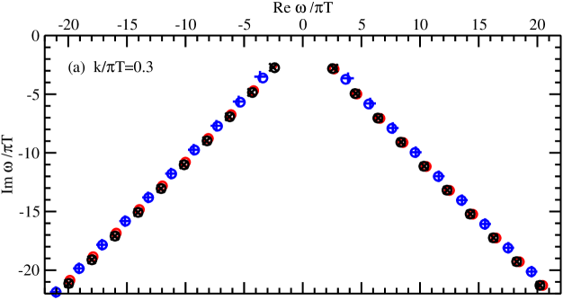
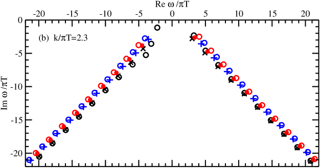
Figure 1: Retarded spin-$\frac{3}{2}$ quasi-normal mode frequencies in the complex $\omega$ plane for $D{=}5$, $mL=\tfrac{3}{2}$, and spin states with ${\bm{\sigma}}\cdot{\bm{\hat{}}{\bm{k}}}=+1$ (as defined in section II). The two figures take (a) $|{\bm{k}}|=0.3\,\pi T$ and (b) $|{\bm{k}}|=2.3\,\pi T$. The figures are not left-right symmetric, and the results for ${\bm{\sigma}}\cdot{\bm{\hat{}}{\bm{k}}}=-1$ are the left-right mirror images of these figures, as required by parity. The open circles are precise numerical results, the small red filled circles show the asymptotic formula (10) for the transverse polarizations, the black $\times$’s show the asymptotic formula (14a) for the first branch of non-transverse solutions, and the blue $+$’s show the asymptotic formula (14b) for the second branch. The latter branch is unphysical for the particular case here since $mL=\tfrac{3}{2}$ is the gravitino case in $D{=}5$, and we have checked numerically that the corresponding blue circles exactly match the quasi-normal modes of the gravitino ghost—a Dirac field with mass $(mL)_{\rm ghost}=\frac{5}{2}$.

I.3.3 Other cases of spin-$\tfrac{3}{2}$ results

In terms of analytic results, this paper focuses on the asymptotic behavior for large $|\omega_{n}|$. For the opposite limit of very small $\omega$ (and ${\bm{k}}$), an analysis of the supersymmetric hydrodynamic mode associated with the gravitino may be found in refs. Policastro ; Erdmenger (see also ref. Gauntlett ).

All of our results assume $D>3$. The special case $D=3$ corresponds to Banados-Teitelboim-Zanelli (BTZ) black holes BTZblackhole , for which exact analytic results are known for quasinormal mode frequencies. For a discussion of results in this case for arbitrary half-integer spin, see ref. BTZdatta .

See refs. gravitino1 ; gravitino2 ; gravitino3 for a variety of analytic and numerical results for gravitino quasinormal modes of $D{=}4$ asymptotically-flat black holes. In contrast, our work here is for asymptotically-AdS black holes, relevant to gauge-gravity duality.

II Review and Improvement of Spin $1/2$ Asymptotic Results

In order to address the spin-$\tfrac{3}{2}$ case, it will be useful to first review the spin-$\tfrac{1}{2}$ case treated in ref. dirac . Here, we will give a treatment that is somewhat simplified compared to ref. dirac and which will be easier to generalize to the spin-$\tfrac{3}{2}$ case. In the process, we will also generalize earlier results to include the $m$ dependence in the argument of the logarithm in the asymptotic result (10).

As reviewed in ref. dirac , the Dirac equation (5) may be rewritten as

$$\left[\sqrt{-g^{tt}}\,\gamma^{t}\partial_{t}+\sqrt{g^{xx}}\,\gamma^{i}\partial_{i}+\sqrt{g^{zz}}\,\gamma^{z}\partial_{z}-m\right]\psi=0,$$ (15)

where the original field $\Psi$ has been rescaled as

$$\Psi\equiv(-gg^{zz})^{-1/4}\psi\propto z^{d/2}f^{-1/4}\psi$$ (16)

and the $\gamma^{m}$ are flat-spacetime $\gamma$ matrices with $\{\gamma^{m},\gamma^{n}\}=2\eta^{mn}$. From now on, we will refer to $\gamma^{z}$ as “$\gamma^{5}$,” just because we find that notation more evocative, but our analysis will nonetheless apply generally to arbitrary dimension $D>3$.

Throughout this paper, our convention for labels for coordinate indices will be that capital letters $M,N,\cdots$ refer to the $D$ curved spacetime dimensions in SAdS_D; Greek letters $\mu,\nu,\cdots$ refer to the $d=D{-}1$ spacetime dimensions parallel to the boundary; the lower-case letters $i,j$ refer to the $d{-}1$ spatial dimensions parallel to the boundary; and lower-case letters $m,n,\cdots$ from roughly the second half of the alphabet refer to the $D$ flat spacetime coordinates of a vielbein, such as appears in the expression $\gamma^{m}$ above.

Multiplying (15) by $-\gamma^{5}\sqrt{-g_{tt}}$, and using the explicit metric (2), we will write the Dirac equation as

$${\cal D}_{1/2}\psi=0,$$ (17a)

where

$${\cal D}_{1/2}\equiv-f\partial_{z}+i\gamma^{5}\gamma^{0}\omega-if^{1/2}\gamma^{5}{\bm{\gamma}}\cdot{\bm{k}}+\bar{m}\,\frac{f^{1/2}}{z}\,\gamma^{5}$$ (17b)

and

$$\bar{m}\equiv mL.$$ (18)

We will find it convenient to work in a particular basis for the $\gamma$ matrices where

$$\gamma^{0}=i\begin{pmatrix}0&\openone\\ \openone&0\end{pmatrix}=i\tau_{1}\otimes\openone,\qquad{\bm{\gamma}}=\begin{pmatrix}{\bm{\sigma}}&0\\ 0&-{\bm{\sigma}}\end{pmatrix}=\tau_{3}\otimes{\bm{\sigma}},\qquad\gamma^{5}=\begin{pmatrix}0&-i\openone\\ i\openone&0\end{pmatrix}=\tau_{2}\otimes\openone,$$ (19)

so that

$${\cal D}_{1/2}=-f\partial_{z}+i\omega\tau_{3}+kf^{1/2}\tau_{1}+\bar{m}\,\frac{f^{1/2}}{z}\,\tau_{2},$$ (20)

where we define

$$k\equiv{\bm{k}}\cdot{\bm{\sigma}}.$$ (21)

We henceforth focus on eigenstates of ${\bm{k}}\cdot{\bm{\sigma}}$, so that

$$k=\pm|{\bm{k}}|.$$ (22)

We define (retarded) quasinormal mode solutions to be solutions that simultaneously (i) vanish at the boundary ($z{=}0$) of SAdS and (ii) are purely infalling at the horizon.

To find the asymptotic quasinormal mode frequencies, we follow ref. dirac and use the Stokes line method nicely reviewed in ref. NatarioSchiappa . Start by taking the naive large-$\omega$ limit of (17), which is

$$\left[-f\partial_{z}+i\omega\tau_{3}\right]\psi\approx 0,$$ (23)

with solution

$$\psi=e^{-i\omega r_{*}\tau_{3}}\eta=e^{-i\omega r_{*}}\eta^{(+)}+e^{+i\omega r_{*}}\eta^{(-)}.$$ (24)

Here $\eta$ is a constant Dirac spinor, $\eta^{(+)}+\eta^{(-)}$ is its decomposition into spinors $\eta^{(\pm)}$ with definite values $\pm$ of $\gamma^{5}\gamma^{0}=\tau_{3}$, and $r_{*}$ is the tortoise coordinate defined by

$$r_{*}=\int_{z}^{\infty}\frac{dz}{f}\,.$$ (25)

As shown, the solution (24) has components that behave as $\exp(\mp i\omega r_{*})$. In order to avoid having one of these component become exponentially small, and so get lost in the approximation error of the other component, we perform WKB by following Stokes lines, defined by $\operatorname{Im}(\omega r_{*})=0$ in the complex $z$ plane. For asymptotic quasinormal mode frequencies, the relevant Stokes lines are depicted qualitatively in fig. 2 in the complex $r$ plane, where $r\equiv L^{2}/z$. To connect the quasinormal mode condition at the boundary of SAdS with the condition at the horizon, we follow the Stokes lines from the boundary at $z{=}0$ to the singularity at $z{=}\infty$ and from there to the horizon at $z{=}z_{\rm h}$. The WKB solution (24) is not valid very close to the boundary or to the singularity (where the $m$ and/or $k$ terms in the Dirac equation become important even for large $\omega$), and so one has to separately solve the Dirac equation in those limiting cases in order to match to the WKB solutions. Far away from the boundary and the singularity, we will refer to the large-$\omega$ WKB solutions (24) along the positive and negative $\omega r_{*}$ Stokes lines as

$$\psi=e^{-i\omega r_{*}\tau_{3}}\eta_{\omega r_{*}>0}=e^{-i\omega r_{*}}\eta^{(+)}_{\omega r_{*}>0}+e^{+i\omega r_{*}}\eta^{(-)}_{\omega r_{*}>0}$$ (26a)

and

$$\psi=e^{-i\omega r_{*}\tau_{3}}\eta_{\omega r_{*}<0}=e^{-i\omega r_{*}}\eta^{(+)}_{\omega r_{*}<0}+e^{+i\omega r_{*}}\eta^{(-)}_{\omega r_{*}<0},$$ (26b)

respectively.

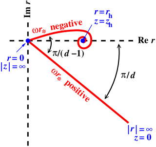
Figure 2: A qualitative picture of the relevant Stokes lines $\operatorname{Im}(\omega r_{*})=0$ in the complex $r$ plane for following WKB between the boundary ($r=\infty$) and the horizon ($r=r_{\rm h}$). The path passes through the singularity ($r=0$) in SAdS_d+1. The other Stokes lines emanating from the origin are not shown, one of which escapes to $-e^{-i\pi/d}\infty$ and the others which spiral into the complex-valued horizons $r=e^{-i2n\pi/d}r_{\rm h}$ for $n=1,\cdots,d{-}1$. (The spiral into the horizon shown above crosses a cut in the definition of $r_{*}$ emanating from $r=r_{\rm h}$, and the curve spirals onto higher and higher Riemann sheets.) Given our retarded convention for $\omega$, this figure is the complex conjugate of similar diagrams in refs. NatarioSchiappa ; CardosoNatarioSchiappa .

Along the negative $\omega r_{*}$ Stokes line of fig. 2, the WKB solution (26b) should have only an $e^{-i\omega r_{*}}$ component, so that it will be purely infalling at the horizon. So $\eta^{(-)}_{\omega r_{*}<0}$ must vanish in (26b). Along the positive $\omega r_{*}$ Stokes line of the figure, the WKB solution will need both $e^{-i\omega r_{*}}$ and $e^{+i\omega r_{*}}$ components in order for $\Psi$ to be able to satisfy the other quasi-normal mode condition that it vanish at the boundary $z{=}0$ of SAdS. The only way both conditions can be satisfied is for the matching near the singularity to mix $e^{-i\omega r_{*}}$ and $e^{+i\omega r_{*}}$ components as one moves from the positive $\omega r_{*}$ Stokes lines to the negative one. Since the naive solution (24) is exact if $k=m=0$, such mixing can only occur if we study the effect of $k$ and $m$ on the solution near the singularity.

In order to study solutions more general than the naive approximation (24), it will be convenient to elevate the $\eta$ in this solution to a function of $z$. Plugging (24) into (17) then recasts the Dirac equation as

$$-fe^{-i\omega r_{*}\tau_{3}}\partial_{z}\eta+f^{1/2}\left(k\tau_{1}+\frac{\bar{m}}{z}\,\tau_{2}\right)e^{-i\omega r_{*}\tau_{3}}\eta=0,$$ (27)

or equivalently

$$\partial_{r_{*}}\eta=-f^{1/2}e^{+2i\omega r_{*}\tau_{3}}\left(k\tau_{1}+\frac{\bar{m}}{z}\,\tau_{2}\right)\eta.$$ (28)

II.1 Behavior near the singularity

Following ref. dirac , we will match WKB solutions between the positive and negative $\omega r_{*}$ Stokes lines of fig. 2 by working in a region that is close enough to the singularity that we may make large-$z$ (small-$r$) approximations, but far enough from the singularity that the $k$ and $m$ terms in the Dirac equation cause only small perturbations to the naive large-$\omega$ solution (24). (See ref. dirac for a detailed justification, which requires $D>3$.) Working in units where $z_{\rm h}=1$ and using the near-singularity approximations

$$f=1-z^{d}\simeq-z^{d},$$ (29)

$$f^{1/2}\simeq-iz^{d/2},$$ (30)

(28) becomes

$$\partial_{r_{*}}\eta\simeq iz^{d/2}e^{+2i\omega r_{*}\tau_{3}}\left(k\tau_{1}+\frac{\bar{m}}{z}\,\tau_{2}\right)\eta.$$ (31)

In earlier work dirac we dropped the $\bar{m}/z$ term compared to the $k$ term, but now we will keep it in order to improve the approximation. (As we will discuss later, this improvement will extend the validity of our asymptotic formula to a wider range of overtone numbers $n$ when $|{\bm{k}}|\ll\bar{m}^{(d-2)/d}T$.) In order to treat $k$ and $\bar{m}$ perturbatively, write

$$\eta(z)=\bar{\eta}+\delta\eta(z),$$ (32)

where $\bar{\eta}$ is constant, and expand to first order in $\delta\eta$, $k$ and $\bar{m}$:

$$\partial_{r_{*}}(\delta\eta)=iz^{d/2}e^{+2i\omega r_{*}\tau_{3}}\left(k\tau_{1}+\frac{\bar{m}}{z}\,\tau_{2}\right)\bar{\eta}.$$ (33)

Then

$$\delta\eta=-i\int_{r_{*}}^{\infty}dr_{*}\>z^{d/2}e^{+2i\omega r_{*}\tau_{3}}\left(k\tau_{1}+\frac{\bar{m}}{z}\,\tau_{2}\right)\bar{\eta}.$$ (34)

Near the singularity, $z$ is related to $r_{*}$ by

$$r_{*}=\int_{z}^{\infty}\frac{dz}{f}\simeq-\frac{1}{(d-1)z^{d-1}},$$ (35)

and so

$$z\simeq\left[e^{-i\pi}(d-1)r_{*}\right]^{-1/(d-1)}.$$ (36)

The result of the $r_{*}$ integration in (34) is then

$$\delta\eta=ike^{-i\pi a}(d-1)^{a-1}\,\frac{\Gamma(a,-2i\omega r_{*}\tau_{3})}{(-2i\omega\tau_{3})^{a}}\,\tau_{1}\bar{\eta}-i\bar{m}e^{i\pi a}(d-1)^{-a}\,\frac{\Gamma(1{-}a,-2i\omega r_{*}\tau_{3})}{(-2i\omega\tau_{3})^{1-a}}\,\tau_{2}\bar{\eta},$$ (37)

where $a$ is defined by (12) and $\Gamma(a,z)$ is the incomplete $\Gamma$ function defined by

$$\Gamma(\alpha,z)=\int_{z}^{\infty}dt\>t^{\alpha-1}e^{-t}.$$ (38)

Now split $\bar{\eta}$ into $\bar{\eta}^{(+)}+\bar{\eta}^{(-)}$ and note that $\tau_{1}\bar{\eta}^{(\pm)}$ and $\tau_{2}\bar{\eta}^{(\pm)}$ have $\tau_{3}=\mp$. So

$$\delta\eta=ike^{-i\pi a}(d-1)^{a-1}\left[\frac{\Gamma(a,-2i\omega r_{*})}{(-2i\omega)^{a}}\,\tau_{1}\bar{\eta}^{(-)}+\frac{\Gamma(a,2i\omega r_{*})}{(2i\omega)^{a}}\,\tau_{1}\bar{\eta}^{(+)}\right]\\ -i\bar{m}e^{i\pi a}(d-1)^{-a}\left[\frac{\Gamma(1{-}a,-2i\omega r_{*})}{(-2i\omega)^{1-a}}\,\tau_{2}\bar{\eta}^{(-)}+\frac{\Gamma(1{-}a,2i\omega r_{*})}{(2i\omega)^{1-a}}\,\tau_{2}\bar{\eta}^{(+)}\right].$$ (39)

In order to match these solutions to WKB expressions along the Stokes lines, we need the asymptotic expansions for $|\omega r_{*}|\gg 1$. The usual formula for the asymptotic expansion of the incomplete Gamma function is

$$\Gamma(\alpha,z)\simeq z^{\alpha-1}e^{-z}\qquad\mbox{($|z|\to\infty$ with $|\arg z|<\frac{3\pi}{2}$)},$$ (40)

giving, for example,

$$\Gamma(a,\pm 2i\omega r_{*})\simeq(\pm 2i\omega r_{*})^{a-1}e^{\pm 2i\omega r_{*}}$$ (41)

and

$$\Gamma(1{-}a,\pm 2i\omega r_{*})\simeq(\pm 2i\omega r_{*})^{-a}e^{\pm 2i\omega r_{*}}$$ (42)

along the positive $\omega r_{*}$ Stokes line. Since $a{-}1$ and $-a$ are negative, these factors and the corresponding $\delta\eta$ (39) vanish as $\omega r_{*}$ becomes large, and so $\eta\to\bar{\eta}$. If the same were true along the negative $\omega r_{*}$ line, then the matching near the singularity would be trivial, with $\eta_{\omega r_{*}>0}=\eta_{\omega r_{*}<0}$ in (26). If that were true, there could be no solution satisfying the boundary conditions required of a quasinormal mode.

The loophole is that the formula (40) does not apply to all the terms of (39) along the negative $\omega r_{*}$ Stokes line. The phase change in $r$ in moving from the positive to the negative $\omega r_{*}$ Stokes line in fig. 2 is $e^{i\pi/(d-1)}$, corresponding to a phase change in $\omega r_{*}$ of $e^{i\pi}$. The phase of $2i\omega r_{*}$ is then $e^{i3\pi/2}$, which violates the condition on the argument $z$ in (40) for the case of $\Gamma(\alpha,2i\omega r_{*})$. We can bring the argument back within the range of validity if we use the monodromy of the incomplete $\Gamma$ function, which is

$$\Gamma(\alpha,e^{i2\pi n}z)=[1-e^{i2\pi n\alpha}]\Gamma(\alpha)+e^{i2\pi n\alpha}\Gamma(\alpha,z).$$ (43)

For our purposes, the differences between the positive $\omega r_{*}$ and negative $\omega r_{*}$ formulas for the asymptotic expansion can be usefully summarized as

$$\Gamma(\alpha,\mp 2i\omega r_{*})\to[\mbox{positive $\omega r_{*}$ formula}]+(1-e^{i2\pi\alpha})\,\Gamma(\alpha)\,\delta_{\mp,+}\,\theta(-\omega r_{*}),$$ (44)

where $\theta$ is the step function. Applying (44) to (39), and remembering that $\eta=\bar{\eta}+\delta\eta$, gives us the relationship between the WKB solutions (26) along the positive and negative $\omega r_{*}$ Stokes lines (to first order in $k$ and $m$):

$$\eta_{\omega r_{*}<0}=\eta_{\omega r_{*}>0}+ike^{-i\pi a}(d-1)^{a-1}\,\frac{(1-e^{i2\pi a})\,\Gamma(a)}{(2i\omega)^{a}}\,\tau_{1}\eta^{(+)}_{\omega r_{*}>0}\\ -i\bar{m}e^{i\pi a}(d-1)^{-a}\,\frac{(1-e^{i2\pi(1-a)})\,\Gamma(1-a)}{(2i\omega)^{1-a}}\,\tau_{2}\eta^{(+)}_{\omega r_{*}>0}.$$ (45)

This may be rewritten in the form

$$\eta_{\omega r_{*}<0}=\eta_{\omega r_{*}>0}+\left(\tau_{1}\lambda\frac{(k/\pi T)}{(\omega/\pi T)^{a}}+\tau_{2}\Lambda\frac{\bar{m}}{(\omega/\pi T)^{1-a}}\,\right)\eta^{(+)}_{\omega r_{*}>0}$$ (46)

where $\lambda$ and $\Lambda$ are defined as in (11), and the temperature $T$ is given by (4).

II.2 Behavior near the boundary

Near the boundary ($z=0$), the SAdS Dirac equation becomes that of pure AdS, corresponding to replacing $f$ by 1 in (17). In our basis (19), the solution which vanishes at the boundary is

$$\psi\propto\sqrt{\pi\Omega z}\begin{pmatrix}J_{\bar{m}-\tfrac{1}{2}}(\Omega z)+i\,\frac{\Omega}{\Omega-k}\,J_{\bar{m}+\tfrac{1}{2}}(\Omega z)\\ \frac{\Omega}{\Omega-k}\,J_{\bar{m}+\tfrac{1}{2}}(\Omega z)+iJ_{\bar{m}-\tfrac{1}{2}}(\Omega z)\end{pmatrix},$$ (47)

where $\Omega^{2}\equiv\omega^{2}-|{\bm{k}}|^{2}$. We’re interested in the limit of large $|\omega|\gg|{\bm{k}}|$. We’re also interested in the asymptotic expansion of this solution away from the boundary (i.e. $\omega z\gg 1$) in order to match to the WKB solution (26a) along the positive $\omega r_{*}$ Stokes line. These further approximations then give

$$\psi\propto\begin{pmatrix}-ie^{-i\bar{m}\pi/2}e^{i\omega z}\\ e^{i\bar{m}\pi/2}e^{-i\omega z}\end{pmatrix}.$$ (48)

For small $z$, the relationship between $z$ and the tortoise coordinate (25) is

$$z\simeq r_{*0}-r_{*},$$ (49)

where

$$r_{*0}\equiv r_{*}\bigl{|}_{\rm boundary}=\int_{0}^{\infty}\frac{dz}{f}=\frac{e^{i\pi/d}}{4T\sin(\pi/d)}\,,$$ (50)

and so

$$\psi\propto e^{-i\omega r_{*}\tau_{3}}\begin{pmatrix}-ie^{-i\bar{m}\pi/2}e^{i\omega r_{*0}}\\ e^{i\bar{m}\pi/2}e^{-i\omega r_{*0}}\end{pmatrix}.$$ (51)

Comparing to (26a), we identify

$$\eta_{\omega r_{*}>0}=C\begin{pmatrix}-ie^{-i\bar{m}\pi/2}e^{i\omega r_{*0}}\\ e^{i\bar{m}\pi/2}e^{-i\omega r_{*0}}\end{pmatrix}\equiv\begin{pmatrix}\eta^{+}_{\omega r_{*}>0}\\[4.0pt] \eta^{-}_{\omega r_{*}>0}\end{pmatrix}$$ (52)

for some proportionality constant $C$. This decomposes into

$$\eta^{(+)}_{\omega r_{*}>0}=\begin{pmatrix}\eta^{+}_{\omega r_{*}>0}\\[4.0pt] 0\end{pmatrix}\qquad\mbox{and}\qquad\eta^{(-)}_{\omega r_{*}>0}=\begin{pmatrix}0\\[4.0pt] \eta^{-}_{\omega r_{*}>0}\end{pmatrix}.$$ (53)

II.3 Putting it together

The horizon condition for the quasi-normal modes is that $\eta^{(-)}_{\omega r_{*}<0}$ vanish, i.e. that there is no $e^{+i\omega r_{*}}$ component of the WKB solution along the negative $\omega r_{*}$ Stokes line of fig. 2. From (46), this condition gives

$$0=\eta^{(-)}_{\omega r_{*}>0}+\left(\tau_{1}\lambda\frac{(k/\pi T)}{(\omega/\pi T)^{a}}+\tau_{2}\Lambda\frac{\bar{m}}{(\omega/\pi T)^{1-a}}\,\right)\eta^{(+)}_{\omega r_{*}>0}$$ (54)

for the WKB coefficients on the positive $\omega r_{*}$ line. In terms of components,

$$0=\eta^{-}_{\omega r_{*}>0}+\left(\lambda\frac{(k/\pi T)}{(\omega/\pi T)^{a}}+i\Lambda\frac{\bar{m}}{(\omega/\pi T)^{1-a}}\,\right)\eta^{+}_{\omega r_{*}>0}.$$ (55)

Using the explicit expression (52) derived from matching the solution along that line to the desired behavior at the boundary $z{=}0$ then gives

$$\left(i\lambda\frac{(k/\pi T)}{(\omega/\pi T)^{a}}-\Lambda\frac{\bar{m}}{(\omega/\pi T)^{1-a}}\,\right)e^{-i\bar{m}\pi}e^{2i\omega r_{*0}}=1.$$ (56)

This condition is satisfied when

$$\ln\left(i\lambda\frac{(k/\pi T)}{(\omega/\pi T)^{a}}-\Lambda\frac{\bar{m}}{(\omega/\pi T)^{1-a}}\,\right)-i\bar{m}\pi+2i\omega r_{*0}=2in\pi$$ (57)

for some integer $n$. Treating $n$ as large, solving for $\omega$ through $O(n^{0})$, and using the explicit expression (50) for $r_{*0}$, gives the result (10) previewed in the introduction.

II.4 Range of validity

The perturbative treatment of $k$ and $m$ near the singularity assumed that the $k$ and $m$ mixing coefficients in (46) were small. Parametrically, that’s

$$\left|\frac{k/T}{(\omega/T)^{a}}\right|\ll 1\qquad\mbox{and}\qquad\left|\frac{\bar{m}}{(\omega/\pi T)^{1-a}}\right|\ll 1.$$ (58)

In terms of the parameter $n\sim|\omega_{n}|/T$ of our asymptotic formula (10), those conditions are equivalent to

$$n\gg\mbox{both}~{}\left(\frac{|{\bm{k}}|}{T}\right)^{1/a}~{}\mbox{and}~{}\bar{m}^{1/(1-a)},$$ (59)

which, for example, for $D{=}5$ would be $n\gg(|{\bm{k}}|/T)^{3}$ and $\bar{m}^{3/2}$. (We will assume for simplicity that $\bar{m}\gtrsim 1$, which is true of fermions coming from compactification of Type II SUGRA on the $S^{5}$ of (S)AdS${}_{5}\times S^{5}$.) In the earlier paper dirac on spin-$\tfrac{1}{2}$ quasinormal modes, we did not include the mass term in the argument of the logarithm in our result (10). The assumption that the $k$ term dominates the $m$ term in the argument of the logarithm requires the additional condition that

$$n\gg\left(\frac{\bar{m}}{|{\bm{k}}|/T}\right)^{1/(1-2a)},$$ (60)

which for $D{=}5$ is $n\gg(\bar{m}T/|{\bm{k}}|)^{3}$. Including the mass term in the logarithm therefore extends the range of validity of our result in those cases where the second condition in (59) is more important than the first—that is, in cases where

$$\frac{|{\bm{k}}|}{T}\ll\bar{m}^{a/(1-a)}=\bar{m}^{(d-2)/d}$$ (61)

(e.g. $|{\bm{k}}|/T\ll\bar{m}^{1/2}$ in $D{=}5$).

III Spin $\tfrac{3}{2}$

III.1 Basic equations

We now turn to the spin-$\tfrac{3}{2}$ equation of motion (6),

$$\Gamma^{MNP}D_{N}\Psi_{P}+m\Gamma^{MN}\Psi_{N}=0.$$ (62)

If $m$ is not the gravitino mass (7), one can show that, in an Einstein spacetime (such as SAdS), this equation implies that

$$\Gamma^{M}\Psi_{M}=0\qquad\mbox{and}\qquad D^{M}\Psi_{M}=0.$$ (63)

If $m$ is the gravitino mass, then there is a gauge symmetry (8), and one may (i) choose $\Gamma^{M}\Psi_{M}=0$ as a gauge condition and (ii) show that the equation of motion then implies $D^{M}\Psi_{M}=0$. In consequence, we will assume (63) in all cases. These conditions allow one to rewrite the equation of motion (62) as

$$\Gamma^{M}D_{M}\Psi_{N}-m\Psi_{N}=0,$$ (64)

supplemented by the constraint that one only keep solutions to (64) that have $\Gamma^{M}\Psi_{M}=0$. Note that (64) differs from the Dirac equation (5) because the covariant derivative in (64) contains a Christoffel term that operates on the vector index $N$ of $\Psi_{N}$.

There are any number of different conventions one might now use to rescale $\Psi$ in order to write out convenient explicit equations in terms of components. We choose the following generalization of the rescaling (16) that we used in the Dirac case:

$$\Psi_{M}\equiv(-gg^{zz})^{-1/4}e^{m}_{M}\psi_{m}\propto z^{d/2}f^{-1/4}e^{m}_{M}\psi_{m},$$ (65)

where $M$ is a curved-space index, $m$ is a flat-space index, and $e^{m}_{M}=\sqrt{|g^{mm}|}\,\delta^{m}_{M}$ (no sum) is the inverse vielbein. With this rewriting, the explicit equations of motion are

$${\cal D}_{1/2}\psi_{0}-\left(\frac{f}{z}-\frac{f^{\prime}}{2}\right)\gamma^{5}\gamma^{0}\psi_{5}=0,$$ (66a)

$${\cal D}_{1/2}\psi_{5}+\frac{f}{z}\psi_{5}+\frac{f^{\prime}}{2}\,\gamma^{5}\gamma^{0}\psi_{0}=0,$$ (66b)

and

$${\cal D}_{1/2}\psi_{i}-\frac{f}{z}\,\gamma^{5}\gamma^{i}\psi_{5}=0.$$ (66c)

Here and throughout, $i=1,\cdots,d-1$ runs over the spatial dimensions parallel to the boundary, “$\psi_{5}$” is our generic notation for the component $\psi_{z}$, and ${\cal D}_{1/2}$ is the same differential operator (17b) as in the spin-$\tfrac{1}{2}$ case.

We are only interested in solutions to (66) which satisfy the constraint $\Gamma^{M}\Psi_{M}=0$, which is equivalent to $\gamma^{m}\psi_{m}=0$. We may use this to determine ${\bm{k}}\cdot{\bm{\psi}}$ in terms of $\Psi_{0}$ and $\Psi_{5}$ as

$${\bm{k}}\cdot{\bm{\psi}} =-\frac{i}{2f^{1/2}}\left[\left(\gamma^{5}{\cal D}_{1/2}-2\bar{m}\frac{f^{1/2}}{z}\right)(-\gamma^{i}\psi_{i})-(d-1)\frac{f}{z}\,\psi_{5}\right]$$

$$=-\frac{i}{2f^{1/2}}\left[\left(\gamma^{5}{\cal D}_{1/2}-2\bar{m}\frac{f^{1/2}}{z}\right)(\gamma^{0}\psi_{0}+\gamma^{5}\psi_{5})-(d-1)\frac{f}{z}\,\psi_{5}\right],$$ (67)

where the first equality follows from the equation of motion (66c) and the explicit form of ${\cal D}_{1/2}$, and the second equality follows from the constraint $\gamma^{m}\psi_{m}=0$.

III.2 “Transverse” solutions

There are two types of solutions to these equations satisfying the constraint. We describe here the first type, which are characterized by $\psi_{5}=0$. We will call such solutions “transverse” polarizations. As noted previously by others Policastro ; Erdmenger , and as we review below, these modes decouple and satisfy a simple Dirac equation. We will see below that they exist only for $D>4$.

From $\psi_{5}{=}0$, it follows by (66b) that $\psi_{0}{=}0$ and thence by (67) that ${\bm{k}}\cdot{\bm{\psi}}=0$ as well. That means that $\psi_{m}$ is zero except for the subset of indices $m$ corresponding to the $D{-}3$ spatial directions parallel to the boundary but transverse to ${\bm{k}}$. For simplicity of presentation, we will focus on the explicit case $D{=}5$ but will state the generalization to larger $D$ at the end. For $D{=}5$, take ${\bm{k}}$ to point in the $x^{3}$ direction. Then, for the transverse solutions under consideration, $\psi_{m}$ is zero except for $\psi_{1}$ and $\psi_{2}$. By the $\gamma$-traceless condition, they must be related by

$$\psi_{2}=-\gamma^{2}\gamma^{1}\psi_{1}.$$ (68)

Since $\psi_{5}=0$, the equation of motion (66c) for both $\psi_{1}$ and $\psi_{2}$ is simply the Dirac equation (17),

$${\cal D}_{1/2}\psi_{i}=0.$$ (69)

So let $\psi_{1}$ be any solution to the Dirac equation. Since $[{\cal D}_{1/2},\gamma^{2}\gamma^{1}]=0$, then $\psi_{2}$ given by (68) will also solve the Dirac equation, and so we have a consistent solution. The quasinormal mode frequencies of these solutions will simply be those of the Dirac equation.

For $D>5$, we can similarly construct transverse solutions by taking only two of the $\psi_{m}$’s non-zero, with those two $m$’s taken from the transverse spatial directions $1,2,\cdots,D{-}3$. One choice of a complete basis of all transverse solutions is to use $\psi_{1}$ and $\psi_{i_{\perp}}$, with $i_{\perp}$ selected from the $D{-}4$ choices $2,3,\cdots,D{-}3$. The quasinormal mode frequencies of transverse solutions are then simply those of the Dirac equation, but with a degeneracy of $D{-}4$ compared to a single Dirac field.

III.3 Setup for finding non-transverse solutions

With the transverse modes out of the way, we will focus exclusively on non-transverse ($\psi_{5}\not=0$) modes in what follows. Because $\psi_{0}$ and $\psi_{5}$ by themselves satisfy a closed set of equations of motion (66a,b), we may ignore what the other components $\psi_{i}$ are doing if our goal is just to find the quasinormal frequencies $\omega_{n}$.

The naive large-$\omega$ limit of the $(\psi_{0},\psi_{5})$ equations of motion (66a,b) is

$$[-f\partial_{z}+i\omega\tau_{3}]\psi_{0}-\left(\frac{f}{z}-\frac{f^{\prime}}{2}\right)\tau_{3}\psi_{5}\simeq 0,$$ (70)

$$[-f\partial_{z}+i\omega\tau_{3}]\psi_{5}+\frac{f}{z}\,\psi_{5}+\frac{f^{\prime}}{2}\,\tau_{3}\psi_{0}=0,$$ (71)

which is the analog to eq. (23) from the spin-$\tfrac{1}{2}$ analysis. The corresponding solution is

$$\begin{pmatrix}\psi_{0}\\ \psi_{5}\end{pmatrix}=\omega zf^{-1/2}e^{-i\omega r_{*}\tau_{3}}\begin{pmatrix}\tau_{3}\left[-\eta+\chi\left(\frac{2f}{z}-\int\frac{f^{\prime}}{z}\right)\right]\\ \eta+\chi\int\frac{f^{\prime}}{z}\end{pmatrix},$$ (72)

where $\eta$ and $\chi$ are arbitrary constant spinors. By convention, we will choose the lower limit on the integrals in (72) to be zero, i.e.

$$\int\frac{f^{\prime}}{z}\equiv\int_{0}^{z}dz_{1}\>\frac{f^{\prime}(z_{1})}{z_{1}}\,.$$ (73)

Similar to our treatment of the spin-$\tfrac{1}{2}$ case, we now promote $\eta$ and $\chi$ to functions of $z$. Plugging (72) into (66a,b) then recasts the exact equations of motion to

$$\partial_{r_{*}}\eta-\left(\frac{2f}{z}-\int\frac{f^{\prime}}{z}\right)\partial_{r_{*}}\chi =f^{1/2}e^{2i\omega r_{*}\tau_{3}}\left(k\tau_{1}+\frac{\bar{m}}{z}\,\tau_{2}\right)\left[\eta-\chi\left(\frac{2f}{z}-\int\frac{f^{\prime}}{z}\right)\right],$$ (74a)

$$\partial_{r_{*}}\eta+\left(\int\frac{f^{\prime}}{z}\right)\partial_{r_{*}}\chi =f^{1/2}e^{2i\omega r_{*}\tau_{3}}\left(k\tau_{1}+\frac{\bar{m}}{z}\,\tau_{2}\right)\left[-\eta-\chi\int\frac{f^{\prime}}{z}\right],$$ (74b)

which may also be written as

$$\partial_{r_{*}}\chi =-f^{1/2}e^{2i\omega r_{*}\tau_{3}}\left(k\tau_{1}+\frac{\bar{m}}{z}\,\tau_{2}\right)\frac{z}{f}\left[\eta-\chi\left(\frac{f}{z}-\int\frac{f^{\prime}}{z}\right)\right],$$ (75a)

$$\partial_{r_{*}}\eta =-\left(\int\frac{f^{\prime}}{z}\right)\partial_{r_{*}}\chi-f^{1/2}e^{2i\omega r_{*}\tau_{3}}\left(k\tau_{1}+\frac{\bar{m}}{z}\,\tau_{2}\right)\left[\eta+\chi\int\frac{f^{\prime}}{z}\right].$$ (75b)

III.4 Behavior near the singularity

Near the singularity, we approximate $f$ by $-z^{d}$ as in the spin-$\tfrac{1}{2}$ case. Then (75) becomes

$$\partial_{r_{*}}\chi \simeq-ie^{2i\omega r_{*}\tau_{3}}\left(k\tau_{1}+\frac{\bar{m}}{z}\,\tau_{2}\right)\left[z^{1-\frac{d}{2}}\eta-\frac{1}{(d-1)}\,z^{\frac{d}{2}}\chi\right],$$ (76)

$$\partial_{r_{*}}\eta \simeq-ie^{2i\omega r_{*}\tau_{3}}\left(k\tau_{1}+\frac{\bar{m}}{z}\,\tau_{2}\right)\left[\frac{1}{(d-1)}\,z^{\frac{d}{2}}\eta+\frac{d(d-2)}{(d-1)^{2}}\,z^{\frac{3d}{2}-1}\chi\right].$$ (77)

Now treat $k$ and $\bar{m}$ as perturbations; take

$$\eta(z)=\bar{\eta}+\delta\eta(z),\qquad\chi(z)=\bar{\chi}+\delta\chi(z);$$ (78)

expand to first order in small quantities; and integrate the resulting equations for $\delta\eta$ and $\delta\chi$ to get

$$\delta\chi =i\int_{r_{*}}^{\infty}dr_{*}\>e^{2i\omega r_{*}\tau_{3}}\left(k\tau_{1}+\frac{\bar{m}}{z}\,\tau_{2}\right)\left[z^{1-\frac{d}{2}}\bar{\eta}-\frac{1}{(d-1)}\,z^{\frac{d}{2}}\bar{\chi}\right],$$ (79)

$$\delta\eta =i\int_{r_{*}}^{\infty}dr_{*}\>e^{2i\omega r_{*}\tau_{3}}\left(k\tau_{1}+\frac{\bar{m}}{z}\,\tau_{2}\right)\left[\frac{1}{(d-1)}\,z^{\frac{d}{2}}\bar{\eta}+\frac{d(d-2)}{(d-1)^{2}}\,z^{\frac{3d}{2}-1}\bar{\chi}\right].$$ (80)

Using (12), (36), and (38), the integration gives

$$\delta\chi =ike^{-i\pi a}(d-1)^{a}\left[\frac{\Gamma(a{+}1,-2i\omega r_{*}\tau_{3})}{(-2i\omega\tau_{3})^{a+1}}\tau_{1}\bar{\eta}+\frac{\Gamma(a,-2i\omega r_{*}\tau_{3})}{(d-1)^{2}(-2i\omega\tau_{3})^{a}}\tau_{1}\bar{\chi}\right]$$

$$+i\bar{m}e^{i\pi a}(d-1)^{1-a}\left[-\frac{\Gamma(2{-}a,-2i\omega r_{*}\tau_{3})}{(-2i\omega\tau_{3})^{2-a}}\tau_{2}\bar{\eta}-\frac{\Gamma(1{-}a,-2i\omega r_{*}\tau_{3})}{(d-1)^{2}(-2i\omega\tau_{3})^{1-a}}\tau_{2}\bar{\chi}\right],$$ (81)

$$\delta\eta =ike^{-i\pi a}(d-1)^{a}\biggl{[}-\frac{\Gamma(a,-2i\omega r_{*}\tau_{3})}{(d-1)^{2}(-2i\omega\tau_{3})^{a}}\tau_{1}\bar{\eta}+\frac{d(d-2)\,\Gamma(a{-}1,-2i\omega r_{*}\tau_{3})}{(d-1)^{4}(-2i\omega\tau_{3})^{a-1}}\tau_{1}\bar{\chi}\biggr{]}$$

$$+i\bar{m}e^{i\pi a}(d-1)^{1-a}\biggl{[}\frac{\Gamma(1{-}a,-2i\omega r_{*}\tau_{3})}{(d-1)^{2}(-2i\omega\tau_{3})^{1-a}}\tau_{2}\bar{\eta}-\frac{d(d-2)\,\Gamma(-a,-2i\omega r_{*}\tau_{3})}{(d-1)^{4}(-2i\omega\tau_{3})^{-a}}\tau_{2}\bar{\chi}\biggr{]}.$$ (82)

Using the monodromy relation (44),

$$\begin{pmatrix}\chi\\ \eta\end{pmatrix}_{\omega r_{*}<0} =\begin{pmatrix}\chi\\ \eta\end{pmatrix}_{\omega r_{*}>0}$$

$$+ike^{-i\pi a}(1-e^{i2\pi a})(d-1)^{a}\begin{pmatrix}\frac{\Gamma(a)}{(d-1)^{2}(2i\omega)^{a}}&\frac{\Gamma(a+1)}{(2i\omega)^{a+1}}\\[6.0pt] \frac{d(d-2)\,\Gamma(a-1)}{(d-1)^{4}(2i\omega)^{a-1}}&-\frac{\Gamma(a)}{(d-1)^{2}(2i\omega)^{a}}\end{pmatrix}\begin{pmatrix}\tau_{1}\chi^{(+)}\\ \tau_{1}\eta^{(+)}\end{pmatrix}_{\omega r_{*}>0}$$

$$+i\bar{m}e^{i\pi a}(1-e^{i2\pi a})(d-1)^{1-a}\begin{pmatrix}-\frac{\Gamma(1-a)}{(d-1)^{2}(2i\omega)^{1-a}}&-\frac{\Gamma(2-a)}{(2i\omega)^{2-a}}\\[6.0pt] -\frac{d(d-2)\,\Gamma(-a)}{(d-1)^{4}(2i\omega)^{-a}}&\frac{\Gamma(1-a)}{(d-1)^{2}(2i\omega)^{1-a}}\end{pmatrix}\begin{pmatrix}\tau_{2}\chi^{(+)}\\ \tau_{2}\eta^{(+)}\end{pmatrix}_{\omega r_{*}>0}.$$ (83)

This can be rewritten as

$$\begin{pmatrix}\chi\\ \eta\end{pmatrix}_{\omega r_{*}<0}=\begin{pmatrix}\chi\\ \eta\end{pmatrix}_{\omega r_{*}>0}+\left[\tau_{1}\lambda\,\frac{k/\pi T}{(\omega/\pi T)^{a}}\utilde{\cal M}+\tau_{2}\Lambda\,\frac{\bar{m}}{(\omega/\pi T)^{1-a}}\utilde{\cal N}\right]\begin{pmatrix}\chi^{(+)}\\ \eta^{(+)}\end{pmatrix}_{\omega r_{*}>0}$$ (84)

with $\lambda$ and $\Lambda$ defined as in (11),

$$\utilde{\cal M}\equiv\begin{pmatrix}\frac{1}{(d-1)}&\frac{(d-1)a}{2i\omega}\\[4.0pt] \frac{d(d-2)2i\omega}{(d-1)^{3}(a-1)}&-\frac{1}{(d-1)}\end{pmatrix},$$ (85)

and

$$\utilde{\cal N}\equiv\begin{pmatrix}\frac{1}{(d-1)}&\frac{(d-1)(1-a)}{2i\omega}\\[4.0pt] \frac{d(d-2)2i\omega}{(d-1)^{3}(-a)}&-\frac{1}{(d-1)}\end{pmatrix}.$$ (86)

In general, we will use undertildes to denote $2\times 2$ matrices that act on the space of $(\chi,\eta)$.

It’s now convenient to simplify using the definition (12) of $a$ and furthermore to rescale the field $\chi$ as

$$\chi=\frac{(d-1)}{4i\omega}\,\hat{\chi},$$ (87)

giving

$$\begin{pmatrix}\hat{\chi}\\ \eta\end{pmatrix}_{\omega r_{*}<0}=\begin{pmatrix}\hat{\chi}\\ \eta\end{pmatrix}_{\omega r_{*}>0}+\left[\tau_{1}\lambda\,\frac{k/\pi T}{(\omega/\pi T)^{a}}\utilde{\hat{\cal M}}+\tau_{2}\Lambda\,\frac{\bar{m}}{(\omega/\pi T)^{1-a}}\utilde{\hat{\cal N}}\right]\begin{pmatrix}\hat{\chi}^{(+)}\\ \eta^{(+)}\end{pmatrix}_{\omega r_{*}>0}$$ (88)

with

$$\utilde{\hat{\cal M}}=\frac{1}{d-1}\begin{pmatrix}1&+(d-2)\\[4.0pt] -(d-2)&-1\end{pmatrix},\qquad\utilde{\hat{\cal N}}=\frac{1}{d-1}\begin{pmatrix}1&+d\\[4.0pt] -d&-1\end{pmatrix}.$$ (89)

The only difference between (88) and the corresponding spin-$\tfrac{1}{2}$ formula (46) is the inclusion of the matrix factors $\utilde{\hat{\cal M}}$ and $\utilde{\hat{\cal N}}$.

III.5 Behavior near the boundary

The desired solutions near the boundary, adapted from ref. Volovich , are

$$\psi_{0}= \pi^{1/2}(\Omega z)^{1/2}\left[\frac{i\gamma^{\mu}k_{\mu}}{\Omega}\,J_{\bar{m}+\frac{1}{2}}(\Omega z)+J_{\bar{m}-\frac{1}{2}}(\Omega z)\right]\xi_{0}$$

$$\quad+\pi^{1/2}(\Omega z)^{3/2}\left[-\frac{k_{0}\gamma^{\mu}k_{\mu}}{\Omega^{2}}\,J_{\bar{m}+\frac{3}{2}}(\Omega z)+\frac{ik_{0}}{\Omega}\,J_{\bar{m}+\frac{1}{2}}(\Omega z)+\frac{\gamma_{0}}{\Omega z}\,J_{\bar{m}+\frac{1}{2}}(\Omega z)\right]\xi_{5},$$ (90)

$$\psi_{5}= \pi^{1/2}(\Omega z)^{3/2}\left[\frac{i\gamma^{\mu}k_{\mu}}{\Omega}\,J_{\bar{m}+\frac{1}{2}}(\Omega z)+J_{\bar{m}-\frac{1}{2}}(\Omega z)\right]\xi_{5},$$ (91)

where $\xi_{0}$ and $\xi_{5}$ are constant spinors that are $\gamma^{5}=+1$ eigenstates of $\gamma^{5}$, and $\Omega\equiv\sqrt{-k^{\mu}k_{\mu}}$. Taking the large $\omega$ limit (with ${\bm{k}}$ fixed) replaces $\Omega$ by $\omega$ above. In our representation (19) for the $\gamma$ matrices, we may write

$$\xi_{I}=\frac{C_{I}}{\sqrt{2}}\begin{pmatrix}-i\\ 1\end{pmatrix}$$ (92)

in the space that the $\tau$ matrices act on, where $C_{0}$ and $C_{5}$ are simple numbers. Taking the asymptotic expansion $\omega z\gg 1$ of (91), one then finds

$$\psi_{0} \simeq\begin{pmatrix}-i(C_{0}-\omega zC_{5})e^{-i\bar{m}\pi/2}e^{i\omega z}\\ (C_{0}+\omega zC_{5})e^{i\bar{m}\pi/2}e^{-i\omega z}\end{pmatrix}\simeq\omega ze^{-i\omega r_{*}\tau_{3}}\tau_{3}\begin{pmatrix}\bigl{(}iC_{5}-\frac{iC_{0}}{\omega z}\bigr{)}e^{-i\bar{m}\pi/2}e^{i\omega r_{*0}}\\[4.0pt] \bigl{(}-C_{5}-\frac{C_{0}}{\omega z}\bigr{)}e^{i\bar{m}\pi/2}e^{-i\omega r_{*0}}\end{pmatrix},$$ (93a)

$$\psi_{5} \simeq\begin{pmatrix}-i\omega zC_{5}e^{-i\bar{m}\pi/2}e^{i\omega z}\\ \omega zC_{5}e^{i\bar{m}\pi/2}e^{-i\omega z}\end{pmatrix}\simeq\omega ze^{-i\omega r_{*}\tau_{3}}\begin{pmatrix}-iC_{5}e^{-i\bar{m}\pi/2}e^{i\omega r_{*0}}\\ C_{5}e^{i\bar{m}\pi/2}e^{-i\omega r_{*0}}\end{pmatrix}.$$ (93b)

Note that we have been slightly inconsistent: We have kept the leading terms for $\omega z\gg 1$ that are proportional to $C_{0}$ and $C_{5}$. However, in (93a), the next-order term proportional to $C_{5}$ would seemingly be the same order in $1/\omega z$ as the leading term proportional to $C_{0}$. However, this will not be an issue in what follows.

We now want to match to the WKB solution (72), which near the boundary becomes

$$\psi_{0} =\omega ze^{-i\omega r_{*}\tau_{3}}\tau_{3}\Bigl{(}-\eta+\frac{2}{z}\,\chi\Bigr{)},$$ (94a)

$$\psi_{5} =\omega ze^{-i\omega r_{*}\tau_{3}}\eta.$$ (94b)

Here again, we are being slightly inconsistent: Corrections to the approximation (72) due to the effects of $\bar{m}$, which were ignored in that equation, could give $O(\bar{m}/z)$ corrections to the $\eta$ term in (94a), which could be parametrically the same size as the $2\chi/z$ term. These corrections are related to the $C_{5}/\omega z$ corrections we ignored in (93a), and we sweep them under the rug here as well.

Comparison of (94) with (93) identifies

$$\eta_{\omega r_{*}>0}=C_{5}\begin{pmatrix}-ie^{-i\bar{m}\pi/2}e^{i\omega r_{*0}}\\ e^{i\bar{m}\pi/2}e^{-i\omega r_{*0}}\end{pmatrix}\equiv\begin{pmatrix}\eta^{+}_{\omega r_{*}>0}\\ \eta^{-}_{\omega r_{*}>0}\end{pmatrix}$$ (95)

and then

$$\chi_{\omega r_{*}>0}=\frac{C_{0}}{2\omega}\begin{pmatrix}-ie^{-i\bar{m}\pi/2}e^{i\omega r_{*0}}\\ -e^{i\bar{m}\pi/2}e^{-i\omega r_{*0}}\end{pmatrix}.$$ (96)

(The net effect of the various corrections that we ignored above can be absorbed into a redefinition of the $C_{0}$ in the last formula—a redefinition which will not be relevant since $C_{0}$ is so far arbitrary.) Using the definition (87) of $\hat{\chi}$,

$$\hat{\chi}_{\omega r_{*}>0}=\hat{C}_{0}\begin{pmatrix}-ie^{-i\bar{m}\pi/2}e^{i\omega r_{*0}}\\ -e^{i\bar{m}\pi/2}e^{-i\omega r_{*0}}\end{pmatrix}\equiv\begin{pmatrix}\hat{\chi}^{+}_{\omega r_{*}>0}\\ \hat{\chi}^{-}_{\omega r_{*}>0}\end{pmatrix},$$ (97)

where $\hat{C}_{0}\equiv 2iC_{0}/(d-1)$.

III.6 Putting it together

The horizon condition for the quasi-normal modes, that there be no $e^{+i\omega r_{*}}$ components at the horizon, requires $\eta^{(-)}$ and $\chi^{(-)}$ to vanish along the $\omega r_{*}<0$ Stokes line. From (88), this condition gives

$$0=\begin{pmatrix}\hat{\chi}^{(-)}\\ \eta^{(-)}\end{pmatrix}_{\omega r_{*}>0}+\left[\lambda\,\frac{k/\pi T}{(\omega/\pi T)^{a}}\tau_{1}\utilde{\hat{\cal M}}+\Lambda\,\frac{\bar{m}}{(\omega/\pi T)^{1-a}}\tau_{2}\utilde{\hat{\cal N}}\right]\begin{pmatrix}\hat{\chi}^{(+)}\\ \eta^{(+)}\end{pmatrix}_{\omega r_{*}>0}.$$ (98)

In terms of components,

$$0=\begin{pmatrix}\hat{\chi}^{-}\\ \eta^{-}\end{pmatrix}_{\omega r_{*}>0}+\left[\lambda\,\frac{k/\pi T}{(\omega/\pi T)^{a}}\utilde{\hat{\cal M}}+i\Lambda\,\frac{\bar{m}}{(\omega/\pi T)^{1-a}}\utilde{\hat{\cal N}}\right]\begin{pmatrix}\hat{\chi}^{+}\\ \eta^{+}\end{pmatrix}_{\omega r_{*}>0}.$$ (99)

Eqs. (95) and (97) then give

$$\left[i\lambda\,\frac{k/\pi T}{(\omega/\pi T)^{a}}\utilde{\hat{\cal M}}-\Lambda\,\frac{\bar{m}}{(\omega/\pi T)^{1-a}}\utilde{\hat{\cal N}}\right]e^{-i\bar{m}\pi}e^{i2\omega r_{*0}}\begin{pmatrix}\hat{C}_{0}\\ C_{5}\end{pmatrix}=\begin{pmatrix}-\hat{C}_{0}\\ C_{5}\end{pmatrix},$$ (100)

and so

$$\left[i\lambda\,\frac{k/\pi T}{(\omega/\pi T)^{a}}\utilde{M}-\Lambda\,\frac{\bar{m}}{(\omega/\pi T)^{1-a}}\utilde{N}\right]e^{-i\bar{m}\pi}e^{i2\omega r_{*0}}\begin{pmatrix}\hat{C}_{0}\\ C_{5}\end{pmatrix}=\begin{pmatrix}\hat{C}_{0}\\ C_{5}\end{pmatrix},$$ (101)

where

$$\utilde{M} \equiv\begin{pmatrix}-1&0\\ 0&1\end{pmatrix}\utilde{\hat{\cal M}}=-\frac{1}{d-1}\begin{pmatrix}1&d{-}2\\[4.0pt] d{-}2&1\end{pmatrix},$$ (102)

$$\utilde{N} \equiv\begin{pmatrix}-1&0\\ 0&1\end{pmatrix}\utilde{\hat{\cal N}}=-\frac{1}{d-1}\begin{pmatrix}1&d\\[4.0pt] d&1\end{pmatrix}.$$ (103)

The quasinormal mode condition is then that

$$\left[i\lambda\,\frac{k/\pi T}{(\omega/\pi T)^{a}}\utilde{M}-\Lambda\,\frac{\bar{m}}{(\omega/\pi T)^{1-a}}\utilde{N}\right]e^{-i\bar{m}\pi}e^{i2\omega r_{*0}}$$ (104)

have an eigenvalue equal to 1. The eigenvectors are

$$\begin{pmatrix}\hat{C}_{0}\\ C_{5}\end{pmatrix}=\begin{pmatrix}1\\ -1\end{pmatrix}~{}\mbox{and}~{}\begin{pmatrix}1\\ 1\end{pmatrix},$$ (105)

and the corresponding conditions are

$$\left[\frac{(d-3)}{(d-1)}\,i\lambda\,\frac{k/\pi T}{(\omega/\pi T)^{a}}-\Lambda\,\frac{\bar{m}}{(\omega/\pi T)^{1-a}}\right]e^{-i\bar{m}\pi}e^{i2\omega r_{*0}}=1$$ (106)

and

$$\left[-i\lambda\,\frac{k/\pi T}{(\omega/\pi T)^{a}}+\frac{(d+1)}{(d-1)}\,\Lambda\,\frac{\bar{m}}{(\omega/\pi T)^{1-a}}\right]e^{-i\bar{m}\pi}e^{i2\omega r_{*0}}=1,$$ (107)

respectively. This is just the spin-$\tfrac{1}{2}$ condition (56) with $\lambda$ and $\Lambda$ replaced by either (i) $(d-3)\lambda/(d-1)$ and $\Lambda$ or (ii) $-\lambda$ and $-(d+1)\Lambda/(d-1)$. Making these substitutions in the Dirac result (10) for the asymptotic quasinormal mode frequencies yields the first and second branch spin-$\tfrac{3}{2}$ results of (14a) and (14b), respectively.

IV Numerics

We would like to compare our analytic asymptotic formulas for quasinormal mode frequencies to precise numerical results. For numerics, we will generalize the method used for the spin-$\tfrac{1}{2}$ case in ref. dirac , which in turn was inspired by methods used by others. We make no claim as to whether our method is the most efficient, but it gets the job done. Here we will focus only on the non-transverse modes, since the transverse ones are described by the Dirac equation and so can be treated numerically by the exact same procedure as ref. dirac . We will start out with a general discussion but will later specialize to the case of $D{=}5$.

IV.1 A 2nd-order equation

Start from the basic equations of motion (75) in terms of $\chi$ and $\eta$, which we write here in the form

$$\partial_{r_{*}}\vec{V}=f^{1/2}e^{2i\omega r_{*}\tau_{3}}\left(k\tau_{1}+\frac{\bar{m}}{z}\,\tau_{2}\right)\utilde{\cal R}\vec{V},$$ (108)

where

$$\vec{V}\equiv\begin{pmatrix}\chi\\ \eta\end{pmatrix},\qquad\utilde{\cal R}\equiv\begin{pmatrix}1-\frac{zg}{f}&-\frac{z}{f}\\[4.0pt] -g(2-\frac{zg}{f})&-(1-\frac{zg}{f})\end{pmatrix}=\utilde{\cal R}^{-1},$$ (109)

and

$$g\equiv\int\frac{f^{\prime}}{z}\,.$$ (110)

In terms of the $\tau_{3}=\pm 1$ components $\chi^{\pm}$ and $\eta^{\pm}$ of the spinors $\chi$ and $\eta$, this is

$$\partial_{r_{*}}\vec{V}^{+} =f^{1/2}e^{2i\omega r_{*}}\left(k-i\,\frac{\bar{m}}{z}\right)\utilde{\cal R}\vec{V}^{-},$$ (111)

$$\partial_{r_{*}}\vec{V}^{-} =f^{1/2}e^{-2i\omega r_{*}}\left(k+i\,\frac{\bar{m}}{z}\right)\utilde{\cal R}\vec{V}^{+},$$ (112)

where

$$\vec{V}^{\pm}\equiv\begin{pmatrix}\chi^{\pm}\\ \eta^{\pm}\end{pmatrix}.$$ (113)

Solving (111) for $\vec{V}^{-}$ and then plugging into (112) gives

$$\partial_{r_{*}}\left[f^{-1/2}e^{-2i\omega r_{*}}\left(k-i\,\frac{\bar{m}}{z}\right)^{-1}\utilde{\cal R}^{-1}\partial_{r_{*}}\vec{V}^{+}\right]=f^{1/2}e^{-2i\omega r_{*}}\left(k+i\,\frac{\bar{m}}{z}\right)\utilde{\cal R}\vec{V}^{+},$$ (114)

which may be rewritten as

$$f\partial_{z}^{2}\vec{V}^{+}+\left(2i\omega+\utilde{\cal S}+\frac{f^{\prime}}{2}-\frac{i\bar{m}f}{z(kz-i\bar{m})}\right)\partial_{z}\vec{V}^{+}-\left(\frac{\bar{m}^{2}}{z^{2}}+k^{2}\right)\vec{V}^{+}=0,$$ (115)

where

$$\utilde{\cal S}\equiv f\utilde{\cal R}^{-1}\partial_{z}({\cal R}^{-1})=\begin{pmatrix}f^{\prime}-g&-1\\ g^{2}+\frac{2ff^{\prime}}{z}-2gf^{\prime}&-(f^{\prime}-g)\end{pmatrix}.$$ (116)

We will find it useful to rewrite this as

$$\utilde{\cal S}=(f^{\prime}-g)\utilde{\Sigma}_{3}-\utilde{\Sigma}_{+}+\left[g^{2}+\frac{2ff^{\prime}}{z}-2gf^{\prime}\right]\utilde{\Sigma}_{-},$$ (117)

where the $\utilde{\Sigma}_{i}$ are Pauli matrices and $\utilde{\Sigma}_{\pm}\equiv\tfrac{1}{2}(\utilde{\Sigma}_{1}\pm i\utilde{\Sigma}_{2})$. For $D=5$,

$$\utilde{\cal S}=-\tfrac{8}{3}\,z^{3}\utilde{\Sigma}_{3}-\utilde{\Sigma}_{+}-8z^{2}(1+\tfrac{1}{9}\,z^{4})\utilde{\Sigma}_{-}.$$ (118)

We now factor out the behavior at the boundary that we do not want for quasinormal modes by rescaling

$$\vec{V}^{+}=z^{-\bar{m}}\vec{H}.$$ (119)

That is, the condition for quasinormal modes is $\vec{H}(0)=0$. Substituting (119) into (115), the equation for $\vec{H}$ is

$$zf\partial_{z}^{2}\vec{H}+\left((2i\omega+\utilde{\cal S})z-2\bar{m}f+\frac{zf^{\prime}}{2}-\frac{i\bar{m}f}{kz-i\bar{m}}\right)\partial_{z}\vec{H}\\ -\left[\frac{\bar{m}^{2}(1-f)}{z}+\bar{m}\left((2i\omega+\utilde{\cal S})+\frac{f^{\prime}}{2}-\frac{kf}{kz-i\bar{m}}\right)+k^{2}z\right]\vec{H}=0.$$ (120)

IV.2 A recursion relation

To implement the correct infalling boundary condition at the horizon, we require $\vec{V}^{+}$ to be regular at the horizon, which will ensure via (72) that the corresponding components of $\psi_{0}$ and $\psi_{5}$ behave like $e^{-i\omega r_{*}}$ at the horizon and not $e^{+i\omega r_{*}}$. So, we take $\vec{V}^{+}$ to have a power series solution around $z=z_{\rm h}$. Working in units where $z_{\rm h}=1$,

$$\vec{H}(z)=\sum_{n=0}^{\infty}\vec{a}_{n}(1-z)^{n}.$$ (121)

By plugging this series into the equation of motion (120), we find a linear recursion relation for the coefficients $\vec{a}_{n}$ of the form

$$\sum_{j=0}^{j_{\rm max}}\utilde{\alpha}_{-j}(n)\,\vec{a}_{n-j}=0,$$ (122)

with the understanding that $\vec{a}_{n}$ vanishes for negative $n$. For $D{=}5$, (122) is a 9-term recursion relation ($j_{\rm max}{=}8$) with explicit coefficients given in appendix B. For $D{=}4$, it is a 7-term recursion relation, also given in the appendix. The $\utilde{\alpha}_{-j}(n)$ above depend on $\omega$, ${\bm{k}}$, and $\bar{m}$.

Solutions exist for arbitrary values of $\vec{a}_{0}$, to which the other coefficients are then linearly related by (122). Define $\utilde{A}_{n}$ by writing

$$\vec{a}_{n}=\utilde{A}_{n}\vec{a}_{0}.$$ (123)

Then $\utilde{A}_{n}$ satisfies the same recursion relation (122) that $\vec{a}_{n}$ does,

$$\sum_{j=0}^{j_{\rm max}}\utilde{\alpha}_{-j}(n)\,\utilde{A}_{n-j}=0,$$ (124a)

initialized by

$$\utilde{A}_{0}=\openone.$$ (124b)

The series solution (121) may then be written as

$$H(z)=\utilde{\cal H}(z)\,\vec{a}_{0}$$ (125)

with

$$\utilde{\cal H}(z)\equiv\sum_{n=0}^{\infty}\utilde{A}_{n}(1-z)^{n}.$$ (126)

A quasinormal mode solution corresponds to $H(1)=0$ for some value of $\vec{a}_{0}$. The existence of such an $\vec{a}_{0}$ is equivalent to the condition that

$$\det\utilde{\cal H}(1)=0.$$ (127)

Our strategy for numerics is to use the recursion relation (124) and series (126), cut off at some suitably high order $n_{\rm max}$, to compute $\det\utilde{\cal H}(1)$ for a given choice of $\omega$ (and fixed $k$ and $\bar{m}$). We then scan the complex $\omega$ plane to find the quasinormal frequencies, corresponding to the zeros of $\det\utilde{\cal H}(1)$. All calculations are carried out with very high precision arithmetic, with the precision and $n_{\rm max}$ increased as necessary to achieve numerical stability and the desired numerical accuracy.

IV.3 Numerical test of asymptotic formulas

We have already shown a comparison of numerical results to asymptotic formulas for quasinormal mode frequencies in fig. 1. In order to perform a more precise comparison, it is useful to focus on the offset $\delta$ from the leading $O(n)$ asymptotic formula, defined by

$$\delta_{n}\equiv\frac{\omega_{n}}{\Delta\omega_{\infty}}-n=\frac{\omega_{n}}{(2-2i)\pi T}-n$$ (128)

for $D{=}5$, where $\Delta\omega_{\infty}$ is the $n{\to}\infty$ spacing between consecutive modes on a given branch. Here we will focus on quasinormal mode frequencies in the right-half complex $\omega$ plane. For the first branch of non-transverse quasinormal mode solutions, fig. 3 shows data points for $\delta_{n}$ from numerics, plotted against dashed lines showing the asymptotic results taken from (14a). The asymptotic formula works very well at large $n$.

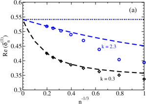
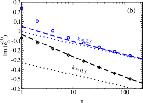
Figure 3: A plot of the (a) real and (b) imaginary parts of the first-branch offsets $\delta_{n}^{(1)}$ defined by (128) for $D=5$, $mL=\tfrac{3}{2}$, $k/\pi T=0.3$ and $2.3$, and the representative overtones $n=1,2,4,8,16,\cdots,128$. Note the different choices made for the horizontal axis in the two figures, and that large $n$ corresponds to the left and right hand sides of (a) and (b) respectively. Data points are from our numerics, whereas the dashed lines indicate the value of $\delta_{n}$ that would be given by the asymptotic formula (14a). Dotted lines are the same formula but dropping the $\bar{m}$ terms in the argument of the logarithms.

The dotted lines in fig. 3 indicate what happens if one were to drop the $\bar{m}$ terms in the argument of the logarithm in the asymptotic formula (14a). We see that including these terms has significantly improved the accuracy for small $k$ and moderate $n$.

Appendix A Gravitino and ghost determinants in $(d{+}1)$-dimensional Einstein spaces

Since one of the possible applications of this work is to compute $1/N_{\rm c}^{2}$ corrections to the free energy of strongly-coupled large-$N_{\rm c}$ ${\cal N}{=}4$ super Yang Mills gauge theory at finite temperature via supergravity loops, in this appendix we show how to account for the gravitino gauge degrees of freedom. More precisely we construct the gravitino and ghost determinants.

To maintain full generality we work in a $(d{+}1)$-dimensional asymptotically AdS space, with the AdS radius denoted by $L$. We begin by decomposing the gravitino field into fields which are divergence-free and gamma-traceless ($\Psi^{\perp}_{M}$), fields which are a pure trace ($\phi$), and fields which reflect the gravitino gauge symmetry ($\zeta$):

$$\Psi_{M}=\Psi_{M}^{\perp}+\frac{1}{d+1}\Gamma_{M}\phi+\Bigl{(}D_{M}-\frac{\Gamma_{M}}{2L}\Bigr{)}\zeta,$$ (129)

where $\Psi_{M}^{\perp}$ obeys

$$D^{M}\Psi_{M}^{\perp}=0,\;\;\;\;\Gamma^{M}\Psi_{M}^{\perp}=0.$$ (130)

(Note that the superscript $\perp$ denotes all divergence-free, gamma-traceless $\Psi_{M}$’s and not just the subset referred to as “transverse” in the main text.) The path integral measure over the spin $3/2$ and $1/2$ fields is defined as

$$\int{\cal D}\Psi_{M}\>\exp\bigg{(}-\int d^{d+1}x\>\sqrt{-g}\,\bar{\Psi}^{M}\Psi_{M}\bigg{)}=1$$ (131)

and

$$\int{\cal D}\phi\>\exp\bigg{(}-\int d^{d+1}x\>\sqrt{-g}\,\bar{\phi}\phi\bigg{)}=1.$$ (132)

The change of integration from $\Psi_{M}$ to $\Psi_{M}^{\perp}$, $\phi$ and $\zeta$ is accompanied by a Jacobian, $Z_{\text{ghost}}$, which can be found from

$$1 = \int{\cal D}\Psi_{M}\>\exp\bigg{(}-\int d^{d+1}x\>\sqrt{-g}\,\bar{\Psi}^{M}\Psi_{M}\bigg{)}$$ (133)

$$= \int{\cal D}\Psi_{M}^{\perp}\int{\cal D}\phi\int{\cal D}\zeta\>Z_{\text{ghost}}\exp\bigg{[}-\bar{\Psi}^{\perp M}\Psi_{M}^{\perp}+\frac{1}{d+1}\bar{\phi}\phi\bigg{]}$$

$$\times\exp\bigg{[}\frac{1}{d+1}\bar{\phi}\Gamma^{M}\Bigl{(}D_{M}-\frac{1}{2L}\Gamma_{M}\Bigr{)}\zeta-\frac{1}{d+1}\,\Bigl{(}D_{M}\bar{\zeta}+\frac{1}{2L}\bar{\zeta}\Gamma_{M}\Bigr{)}\Gamma^{M}\phi\bigg{]}$$

$$\times\exp\bigg{[}-\Bigl{(}D_{M}\bar{\zeta}+\frac{1}{2L}\bar{\zeta}\Gamma_{M}\Bigr{)}\Bigl{(}D^{M}-\frac{1}{2L}\Gamma^{M}\Bigr{)}\zeta\bigg{]},$$

where we introduced the notation

$$D_{M}\bar{\zeta}=\partial_{M}\bar{\zeta}-\frac{1}{4}\bar{\zeta}\omega_{M}^{mn}\gamma^{mn}.$$ (134)

After a further redefinition with unit Jacobian

$$\phi^{\prime}=\phi+\Gamma^{M}\Bigl{(}D_{M}-\frac{1}{2L}\Gamma_{M}\Bigr{)}\zeta$$ (135)

and after performing some of the integrals in (133) we are left with

$$1=\int{\cal D}\zeta\>Z_{\text{ghost}}\exp\bigg{[}-\Bigl{(}D_{M}\bar{\zeta}-\frac{1}{d+1}D_{N}\bar{\zeta}\Gamma^{N}\Gamma_{M}\Bigr{)}\Bigl{(}D^{M}\zeta-\frac{1}{d+1}\Gamma^{M}\Gamma^{P}D_{P}\zeta\Bigr{)}\bigg{]}.$$ (136)

After integration by parts, some Dirac algebra manipulations together with $[D_{M},D_{N}]\zeta=\tfrac{1}{4}R_{MNpq}\gamma^{pq}\zeta$ and $R_{MN}=-\tfrac{d}{L^{2}}g_{MN}$, (136) yields

$$1=\int{\cal D}\zeta\>Z_{\text{ghost}}\exp\bigg{[}\frac{d}{d+1}\bigg{(}\bar{\zeta}D^{M}D_{M}\zeta-\frac{d+1}{4L^{2}}\bar{\zeta}\zeta\bigg{)}\bigg{]}.$$ (137)

The Jacobian (ghost determinant) is now determined to be

$$Z_{\text{ghost}}=\frac{1}{\text{det}_{\tfrac{1}{2}}(D^{M}D_{M}-\frac{d+1}{4L^{2}})},$$ (138)

where the subscript $\tfrac{1}{2}$ in the above expression is meant to express that the operator $D^{M}D_{M}-\frac{d+1}{4}$ acts on spin-$\tfrac{1}{2}$ fields.

On the other hand, integrating out the gravitino from its quadratic action yields

$$Z_{\text{gravitino}} \propto \int{\cal D}\Psi_{M}\>\exp\bigg{[}\int d^{d+1}x\>\sqrt{-g}\,\bar{\Psi}_{M}\Bigl{(}\Gamma^{MNP}D_{N}\Psi_{P}+\frac{d-1}{2L}\Gamma^{MN}\Psi_{N}\Bigr{)}\bigg{]}$$

$$= \int{\cal D}\Psi^{\perp}_{M}\int{\cal D}\phi\int{\cal D}\zeta\>Z_{\text{ghost}}\exp\bigg{[}\int d^{d+1}x\>\sqrt{-g}\,\bar{\Psi}_{M}^{\perp}\Bigr{(}\Gamma^{N}D_{N}-\frac{d-1}{2L}\Bigr{)}\Psi_{M}^{\perp}\bigg{]}$$

$$\qquad\times\exp\bigg{[}-\frac{d(d-1)}{(d+1)^{2}}\int d^{d+1}x\>\sqrt{-g}\,\bar{\phi}\Bigl{(}\Gamma^{M}D_{M}+\frac{d+1}{2L}\Bigr{)}\phi\bigg{]}$$

Throwing away the volume of the gauge group yields

$$Z_{\text{gravitino}}=\frac{\text{det}_{\tfrac{3}{2},\perp}(\Gamma^{M}D_{M}-\frac{d-1}{2L})\;\text{det}_{\tfrac{1}{2}}(\Gamma^{M}D_{M}+\frac{d+1}{2L})}{\text{det}_{\tfrac{1}{2}}(D^{M}D_{M}-\frac{d+1}{4L^{2}})},$$ (140)

where the $\text{det}_{\tfrac{3}{2},\perp}$ denotes the evaluation of the determinant on the subspace of spin-$\tfrac{3}{2}$ fields which are divergence-free and gamma-traceless.

The gravitino partition function can be rewritten in a more compact form by using the same sort of manipulations as before to see that

$$\text{det}_{\tfrac{1}{2}}(D^{M}D_{M}-\tfrac{d+1}{4L^{2}})=\text{det}_{\tfrac{1}{2}}(\Gamma^{M}D_{M}+\tfrac{d+1}{2L})\;\text{det}_{\tfrac{1}{2}}(\Gamma^{M}D_{M}-\tfrac{d+1}{2L})$$ (141)

and so

$$Z_{\text{gravitino}}=\frac{\text{det}_{\tfrac{3}{2},\perp}(\Gamma^{M}D_{M}-\frac{d-1}{2L})}{\text{det}_{\tfrac{1}{2}}(\Gamma^{M}D_{M}-\frac{d+1}{2L})}\,.$$ (142)

Now recall from the main text that one of the branches of the gravitino quasinormal modes had the same frequencies as the ghost quasinormal modes. The form (142) shows that, if one writes each determinant following Denef-Hartnoll-Sachdev as a product of factors involving quasinormal frequencies DHS , then the contributions from this branch will exactly cancel the ghost determinant.

Appendix B Recursion coefficients ${\alpha}_{-j}(n)$

B.1 $D=5$

For $D{=}5$, the results for the coefficients of the recursion relation (122) are

$$\utilde{\alpha}_{-j}(n)=\alpha_{-j}^{0}(n)\,\utilde{\openone}+\alpha_{-j}^{3}(n)\,\utilde{\Sigma}_{3}+\alpha_{-j}^{+}(n)\,\utilde{\Sigma}_{+}+\alpha_{-j}^{-}(n)\,\utilde{\Sigma}_{-},$$ (143)

where $\alpha_{-j}^{0}$ are the same as the coefficients for the spin-$\tfrac{1}{2}$ case dirac ,

$$\alpha_{-6}^{0} =\alpha_{-7}^{0}=\alpha_{-8}^{0}=0,$$ (144a)

$$\alpha_{-5}^{0} =-(4+\bar{m}-n)(5+\bar{m}-n)k,$$ (144b)

$$\alpha_{-4}^{0} =(4+\bar{m}-n)\bigl{[}(20+4\bar{m}-6n)k+(-2-\bar{m}+n)i\bar{m}\bigr{]},$$ (144c)

$$\alpha_{-3}^{0} =(-120-54\bar{m}-6\bar{m}^{2}+85n+20\bar{m}n-15n^{2})k-k^{3}$$

$$\qquad+(24+18\bar{m}+3\bar{m}^{2}-23n-8\bar{m}n+5n^{2})i\bar{m},$$ (144d)

$$\alpha_{-2}^{0} =(80+36\bar{m}+4\bar{m}^{2}-80n-20\bar{m}n+20n^{2})k+2k^{3}$$

$$\qquad+(-24-18\bar{m}-3\bar{m}^{2}+32n+12\bar{m}n-10n^{2})i\bar{m}-ik^{2}\bar{m}+(4+2\bar{m}-2n)ik\omega,$$ (144e)

$$\alpha_{-1}^{0} =(-18-6\bar{m}-\bar{m}^{2}+32n+8\bar{m}n-14n^{2})k-k^{3}$$

$$\qquad+(8+6\bar{m}+\bar{m}^{2}-18n-8\bar{m}n+10n^{2})i\bar{m}$$

$$\qquad+ik^{2}\bar{m}+(-2-2\bar{m}+2n)\bar{m}\omega+(-4-2\bar{m}+4n)ik\omega,$$ (144f)

$$\alpha_{0}^{0} =2n(k-i\bar{m})(-1+2n-i\omega),$$ (144g)

and the others are

$$\alpha_{-6}^{3} =\alpha_{-7}^{3}=\alpha_{-8}^{3}=0,$$ (145a)

$$\alpha_{-5}^{3} =\tfrac{8}{3}(5+\bar{m}-n)k,$$ (145b)

$$\alpha_{-4}^{3} =-\tfrac{8}{3}(20+4\bar{m}-5n)k+\tfrac{8}{3}(4+\bar{m}-n)i\bar{m},$$ (145c)

$$\alpha_{-3}^{3} =\tfrac{16}{3}(15+3\bar{m}-5n)k-\tfrac{8}{3}(12+3\bar{m}-4n)i\bar{m},$$ (145d)

$$\alpha_{-2}^{3} =-\tfrac{16}{3}(10+2\bar{m}-5n)k+8(4+\bar{m}-2n)i\bar{m},$$ (145e)

$$\alpha_{-1}^{3} =\tfrac{8}{3}(5+\bar{m}-5n)k-\tfrac{8}{3}(4+\bar{m}-4n)i\bar{m},$$ (145f)

$$\alpha_{0}^{3} =\tfrac{8}{3}\,n(k-i\bar{m}),$$ (145g)

and

$$\alpha_{-3}^{+} =\alpha_{-4}^{+}=\alpha_{-5}^{+}=\alpha_{-6}^{0}=\alpha_{-7}^{0}=\alpha_{-8}^{0}=0,$$ (146a)

$$\alpha_{-2}^{+} =-(2+\bar{m}-n)k,$$ (146b)

$$\alpha_{-1}^{+} =(2+\bar{m}-2n)k-(1+\bar{m}-n)i\bar{m},$$ (146c)

$$\alpha_{0}^{+} =n(k-i\bar{m}),$$ (146d)

and

$$\alpha_{-8}^{-} =-\tfrac{8}{9}(8+\bar{m}-n)k,$$ (147a)

$$\alpha_{-7}^{-} =\tfrac{8}{9}(56+7\bar{m}-8n)k-\tfrac{8}{9}(7+\bar{m}-n)i\bar{m},$$ (147b)

$$\alpha_{-6}^{-} =-\tfrac{56}{9}(24+3\bar{m}-4n)k+\tfrac{8}{9}(42+6\bar{m}-7n)i\bar{m},$$ (147c)

$$\alpha_{-5}^{-} =\tfrac{56}{9}(40+5\bar{m}-8n)k-\tfrac{8}{3}(35+5\bar{m}-7n)i\bar{m},$$ (147d)

$$\alpha_{-4}^{-} =-\tfrac{8}{9}(316+44\bar{m}-79n)k+\tfrac{40}{9}(28+4\bar{m}-7n)i\bar{m},$$ (147e)

$$\alpha_{-3}^{-} =\tfrac{32}{9}(69+12\bar{m}-23n)k-\tfrac{32}{9}(33+6\bar{m}-11n)i\bar{m},$$ (147f)

$$\alpha_{-2}^{-} =-\tfrac{16}{9}(82+17\bar{m}-41n)k+\tfrac{64}{3}(4+\bar{m}-2n)i\bar{m},$$ (147g)

$$\alpha_{-1}^{-} =\tfrac{16}{9}(22+5\bar{m}-22n)k-\tfrac{16}{9}(17+5\bar{m}-17n)i\bar{m},$$ (147h)

$$\alpha_{0}^{-} =\tfrac{80}{9}\,n(k-i\bar{m}).$$ (147i)

Note that this is a 9-term recursion relation, whereas the spin-$\tfrac{1}{2}$ case dirac gave a 6-term recursion relation. We are unsure if some clever change of variables could yield simpler recursion relations.

B.2 $D=4$

For the sake of completeness, we also give here the recursion coefficients for the case of $D{=}4$. The $\alpha_{-j}^{0}$ are again the same as the coefficients for the spin-$\tfrac{1}{2}$ case, which are

$$\alpha_{-6}^{0} =\alpha_{-5}^{0}=0,$$ (148a)

$$\alpha_{-4}^{0} =\tfrac{1}{2}(7+2\bar{m}-2n)(4+\bar{m}-n)k,$$ (148b)

$$\alpha_{-3}^{0} =\tfrac{1}{2}(-84-45\bar{m}-6\bar{m}^{2}+58n+16\bar{m}n-10n^{2})k-k^{3}$$

$$\qquad+\tfrac{1}{2}(3+2\bar{m}-2n)(3+\bar{m}-n)i\bar{m},$$ (148c)

$$\alpha_{-2}^{0} =\tfrac{1}{2}(84+45\bar{m}+6\bar{m}^{2}-82n-24\bar{m}n+20n^{2})k+2k^{3}$$

$$\qquad-\tfrac{1}{2}(18+18\bar{m}+4\bar{m}^{2}-25n-12\bar{m}n+8n^{2})i\bar{m}-ik^{2}\bar{m}+(4+2\bar{m}-2n)ik\omega,$$ (148d)

$$\alpha_{-1}^{0} =\tfrac{1}{2}(-24-9\bar{m}-2\bar{m}^{2}+42n+12\bar{m}n-18n^{2})k-k^{3}$$

$$\qquad+\tfrac{1}{2}(9+9\bar{m}+2\bar{m}^{2}-21n-12\bar{m}n+12n^{2})i\bar{m}$$

$$\qquad+ik^{2}\bar{m}+(-2-2\bar{m}+2n)\bar{m}\omega+(-4-2\bar{m}+4n)ik\omega,$$ (148e)

$$\alpha_{0}^{0} =\tfrac{1}{2}n(k-i\bar{m})(-3+6n-4i\omega).$$ (148f)

The other coefficients are

$$\alpha_{-5}^{3} =\alpha_{-6}^{3}=0,$$ (149a)

$$\alpha_{-4}^{3} =-\tfrac{3}{2}(4+\bar{m}-n)k,$$ (149b)

$$\alpha_{-3}^{3} =\tfrac{3}{2}(12+3\bar{m}-4n)k-\tfrac{3}{2}(3+\bar{m}-n)i\bar{m},$$ (149c)

$$\alpha_{-2}^{3} =-\tfrac{9}{2}(4+\bar{m}-2n)k+\tfrac{3}{2}(6+2\bar{m}-3n)i\bar{m},$$ (149d)

$$\alpha_{-1}^{3} =\tfrac{3}{2}(4+\bar{m}-4n)k-\tfrac{3}{2}(3+\bar{m}-3n)i\bar{m},$$ (149e)

$$\alpha_{0}^{3} =\tfrac{3}{2}\,n(k-i\bar{m}),$$ (149f)

and

$$\alpha_{-3}^{+} =\alpha_{-4}^{+}=\alpha_{-5}^{+}=\alpha_{-6}^{0}=0,$$ (150a)

$$\alpha_{-2}^{+} =-(2+\bar{m}-n)k,$$ (150b)

$$\alpha_{-1}^{+} =(2+\bar{m}-2n)k-(1+\bar{m}-n)i\bar{m},$$ (150c)

$$\alpha_{0}^{+} =n(k-i\bar{m}),$$ (150d)

and

$$\alpha_{-6}^{-} =-\tfrac{3}{4}(6+\bar{m}-n)k,$$ (151a)

$$\alpha_{-5}^{-} =\tfrac{3}{4}(30+5\bar{m}-6n)k-\tfrac{3}{4}(5+\bar{m}-n)i\bar{m},$$ (151b)

$$\alpha_{-4}^{-} =-\tfrac{15}{4}(12+2\bar{m}-3n)k+\tfrac{3}{4}(20+4\bar{m}-5n)i\bar{m},$$ (151c)

$$\alpha_{-3}^{-} =\tfrac{3}{2}(42+9\bar{m}-14n)k-\tfrac{3}{2}(15+3\bar{m}-5n)i\bar{m},$$ (151d)

$$\alpha_{-2}^{-} =-\tfrac{9}{4}(26+7\bar{m}-13n)k+\tfrac{9}{2}(6+2\bar{m}-3n)i\bar{m},$$ (151e)

$$\alpha_{-1}^{-} =\tfrac{9}{4}(10+3\bar{m}-10n)k-\tfrac{9}{4}(7+3\bar{m}-7n)i\bar{m},$$ (151f)

$$\alpha_{0}^{-} =\tfrac{27}{4}\,n(k-i\bar{m}).$$ (151g)

This is a 7-term recursion relation.

References

- (1) F. Denef, S. A. Hartnoll and S. Sachdev, “Black hole determinants and quasinormal modes,” Class. Quant. Grav. 27, 125001 (2010) [arXiv:0908.2657 [hep-th]].
- (2) S. S. Gubser, I. R. Klebanov and A. A. Tseytlin, “Coupling constant dependence in the thermodynamics of N=4 supersymmetric Yang-Mills theory,” Nucl. Phys. B 534, 202 (1998) [hep-th/9805156].
- (3) R. C. Myers, M. F. Paulos and A. Sinha, “Quantum corrections to ,” Phys. Rev. D 79, 041901 (2009) [arXiv:0806.2156 [hep-th]].
- (4) E. Berti, V. Cardoso and A. O. Starinets, “Quasinormal modes of black holes and black branes,” Class. Quant. Grav. 26, 163001 (2009) [arXiv:0905.2975 [gr-qc]].
- (5) R. A. Konoplya and A. Zhidenko, “Quasinormal modes of black holes: From astrophysics to string theory,” Rev. Mod. Phys. 83, 793 (2011) [arXiv:1102.4014 [gr-qc]].
- (6) P. Arnold and P. Szepietowski, “Spin 1/2 quasinormal mode frequencies in Schwarzschild-AdS spacetime,” arXiv:1308.0341 [hep-th].
- (7) S. Deser and B. Zumino, “Broken Supersymmetry and Supergravity,” Phys. Rev. Lett. 38, 1433 (1977).
- (8) S. Corley, “The Massless gravitino and the AdS / CFT correspondence,” Phys. Rev. D 59, 086003 (1999) [hep-th/9808184].
- (9) A. S. Koshelev and O. A. Rytchkov, “Note on the massive Rarita-Schwinger field in the AdS / CFT correspondence,” Phys. Lett. B 450, 368 (1999) [hep-th/9812238].
- (10) P. Matlock and K. S. Viswanathan, “The AdS / CFT correspondence for the massive Rarita-Schwinger field,” Phys. Rev. D 61, 026002 (1999) [hep-th/9906077].
- (11) H. J. Kim, L. J. Romans and P. van Nieuwenhuizen, “Mass spectrum of chiral ten-dimensional Supergravity on ,” Phys. Rev. D 32, 389 (1985).
- (12) P. K. Townsend, “Cosmological Constant in Supergravity,” Phys. Rev. D 15, 2802 (1977).
- (13) B. de Wit and I. Herger, “Anti-de Sitter supersymmetry,” Lect. Notes Phys. 541, 79 (2000) [hep-th/9908005].
- (14) O. Aharony, S. S. Gubser, J. M. Maldacena, H. Ooguri and Y. Oz, “Large N field theories, string theory and gravity,” Phys. Rept. 323, 183 (2000) [hep-th/9905111].
- (15) M. Giammatteo and J. Jing, “Dirac quasinormal frequencies in Schwarzschild-AdS space-time,” Phys. Rev. D 71, 024007 (2005) [gr-qc/0403030].
- (16) G. Policastro, “Supersymmetric hydrodynamics from the AdS/CFT correspondence,” JHEP 0902, 034 (2009) [arXiv:0812.0992 [hep-th]].
- (17) J. Erdmenger and S. Steinfurt, “A universal fermionic analogue of the shear viscosity,” JHEP 1307, 018 (2013) [arXiv:1302.1869 [hep-th]].
- (18) J. P. Gauntlett, J. Sonner and D. Waldram, “Spectral function of the supersymmetry current,” JHEP 1111, 153 (2011) [arXiv:1108.1205 [hep-th]].
- (19) M. Banados, C. Teitelboim and J. Zanelli, “The Black hole in three-dimensional space-time,” Phys. Rev. Lett. 69, 1849 (1992) [hep-th/9204099].
- (20) S. Datta and J. R. David, “Higher spin fermions in the BTZ black hole,” JHEP 1207, 079 (2012) [arXiv:1202.5831 [hep-th]].
- (21) H. Onozawa, T. Okamura, T. Mishima and H. Ishihara, “Perturbing supersymmetric black hole,” Phys. Rev. D 55, 4529 (1997) [gr-qc/9606086].
- (22) H. T. Cho, “Asymptotic quasinormal frequencies of different spin fields in spherically symmetric black holes,” Phys. Rev. D 73, 024019 (2006) [gr-qc/0512052].
- (23) Q. -Y. Pan and J. -L. Jing, “Quasinormal modes of the Schwarzschild black hole with arbitrary spin fields: Numerical analysis,” Mod. Phys. Lett. A 21, 2671 (2006).
- (24) J. Natario and R. Schiappa, “On the classification of asymptotic quasinormal frequencies for -dimensional black holes and quantum gravity,” Adv. Theor. Math. Phys. 8, 1001 (2004) [hep-th/0411267].
- (25) V. Cardoso, J. Natario and R. Schiappa, “Asymptotic quasinormal frequencies for black holes in nonasymptotically flat space-times,” J. Math. Phys. 45, 4698 (2004) [hep-th/0403132].
- (26) A. Volovich, “Rarita-Schwinger field in the AdS/CFT correspondence,” JHEP 9809, 022 (1998) [hep-th/9809009].
- (27) H.-b. Zhang and X. Zhang, “One loop partition function from normal modes for supergravity in AdS3,” Class. Quant. Grav. 29, 145013 (2012) [arXiv:1205.3681 [hep-th]].
- (28) J. R. David, M. R. Gaberdiel and R. Gopakumar, “The Heat Kernel on AdS(3) and its Applications,” JHEP 1004, 125 (2010) [arXiv:0911.5085 [hep-th]].