Generation and stabilization of a three-qubit entangled W state in circuit QED via quantum feedback control

Abstract

Circuit cavity quantum electrodynamics (QED) is proving to be a powerful platform to implement quantum feedback control schemes due to the ability to control superconducting qubits and microwaves in a circuit. Here, we present a simple and promising quantum feedback control scheme for deterministic generation and stabilization of a three-qubit $W$ state in the superconducting circuit QED system. The control scheme is based on continuous joint Zeno measurements of multiple qubits in a dispersive regime, which enables us not only to infer the state of the qubits for further information processing but also to create and stabilize the target $W$ state through adaptive quantum feedback control. We simulate the dynamics of the proposed quantum feedback control scheme using the quantum trajectory approach with an effective stochastic maser equation obtained by a polaron-type transformation method and demonstrate that in the presence of moderate environmental decoherence, the average state fidelity higher than $0.9$ can be achieved and maintained for a considerable long time (much longer than the single-qubit decoherence time). This control scheme is also shown to be robust against measurement inefficiency and individual qubit decay rate differences. Finally, the comparison of the polaron-type transformation method to the commonly used adiabatic elimination method to eliminate the cavity mode is presented.

I Introduction

Entanglement is regarded as one of the key resources for various applications in quantum information processing. While entanglement of bipartite systems is well understood Peres (1996), the characterization of multipartite entanglement is still an interesting research topic. It has been shown Dür et al. (2000) that there are two inequivalent non-biseparable classes of three-qubit entanglement states, the Greenberger-Horne-Zeilinger (GHZ)class and the W class, which cannot be transformed into each other by stochastic local operations and classical communications. The W state is central as a resource in quantum information processing and multi-party quantum communication as its entanglement is persistent and robust even under particle loss Dür et al. (2000); Gühne et al. (2008); Briegel and Raussendorf (2001). The three-qubit entangled W state has been experimentally generated and demonstrated in systems of trapped ions Haffner et al. (2005), optical photons Eibl et al. (2004), superconducting phase qubits Neeley et al. (2010), and coupled nonlinear oscillator arrays Gangat13 .

Circuit QED system Blais et al. (2004); Wallraff et al. (2004, 2005); Schuster et al. (2005); Gambetta et al. (2006); Blais et al. (2007); Gambetta et al. (2007); Houck et al. (2008); Bonzom2008 ; Boissonneault et al. (2009); Filipp et al. (2009); DiCarlo et al. (2010); Chow et al. (2010); Leek et al. (2010); Filipp et al. (2011); DiCarlo09 ; Reed12 ; Fedorov12 in which superconducting qubits based on Josephson junctions are coupled to a high-Q microwave transmission line resonator acting as a quantum bus has been demonstrated to be a promising solid-state quantum computing architecture. Due to the great controllability of the superconducting qubits and microwaves in the circuit system, the circuit QED system, a solid-state analogy of quantum optics cavity QED, also has excellent potential as a platform for quantum control–especially quantum feedback control–experiments Nadav08 ; Vijay2011 ; Vijay2012 ; Murch12 ; Murch1301 ; Murch1305 ; Riste13 . In this paper, we present a simple and promising quantum feedback control scheme for deterministic generation and stabilization of a three-qubit $W$ state in the superconducting circuit QED system.

Generation and manipulation of entangled states are important tasks of quantum information processing. Besides the scheme based on unitary dynamics to generate entangled states Neeley et al. (2010); Ferber and Wilhelm (2010); Spilla2012 , there are proposals of entanglement generation by measurement Helmer and Marquardt (2009); Bishop2009 ; Lalumière et al. (2010). Although measurements can generate entangled states that are otherwise difficult to obtain, the specific or target entangled states created are primarily probabilistic. Furthermore, the measurement-alone approach cannot stabilize and protect the generated entangled states from deterioration.

One possible way to resolve this problem is to employ the technique of quantum feedback control Wiseman and Milburn (1993); Wiseman09 ; Carvalho and Hope (2007); Sarovar05 ; Tornberg and Johansson (2010); Liu et al. (2010); Feng et al. (2011). There have been proposals of using quantum feedback control to stabilize and generate two-qubit Bell states in circuit QED Sarovar05 ; Liu et al. (2010); Keane12 . Ristè et al. Riste13 recently presented an experimental demonstration of a superconducting two-qubit Bell state produced by feedback based on parity measurements. The case for three-qubit entangled GHZ in circuit QED has also been investigated Feng et al. (2011), but a somewhat complicated method of an alternate-flip-interrupted Zeno scheme and quantum feedback control technique with efficient measurement and rapid single-qubit rotations are required to produce and maintain the pre-GHZ state with high fidelity. However, how to generate and stabilize the other inequivalent class of three-qubit states, namely the W state, in circuit QED has, to our knowledge, not been reported.

Here, we present a simple measurement and feedback control scheme that is feasible with current circuit QED technology to produce and stabilize the W state of $\left|W^{-}\right\rangle=(|100\rangle+|010\rangle+|001\rangle)/\sqrt{3}$. Our scheme does not assume fast single-qubit rotations and is robust against measurement inefficiency and individual qubit decay rate differences. A successful experimental implementation and realization of using quantum feedback control to generate and stabilize a multi-qubit entangled W state as presented here will be an impressive demonstration in circuit QED experiments. Moreover, previous investigations were performed in a parameter regime of a strongly damped resonator cavity so that one can adiabatically eliminate the cavity mode by enslaving the cavity to qubit dynamics Milburn et al. (1994); Brun and Goan (2003); Wang et al. (2005); Sarovar05 ; Liu et al. (2010). Here, we go beyond this so-called bad-cavity limit by using a polaron-type transformation Gambetta et al. (2008); Lalumière et al. (2010) to trace out the cavity mode in our analysis. This allows us to work in a parameter regime in which the W state can be maintained with higher fidelity. The obtained effective (stochastic) master equation for the qubit degrees of freedom provides us with more intuitive understanding and physical insight into the qubit dynamics of the continuous quantum measurement and quantum feedback control process. Note that our method can be extended straightforwardly to the generation and stabilization of a $N$-qubit W-type state that is a quantum superposition with equal expansion coefficients of all possible pure states in which exactly one of the qubits is in an excited state $|1\rangle$, while all other ones are in the ground state $|0\rangle$.

The paper is organized as follows. We describe a three-qubit circuit QED setup and its corresponding model Hamiltonian in Sec. II. The procedure of using polaron-type transformation to eliminate cavity field to obtain an effective master equation for the qubit degrees of freedom alone conditioned on continuous homodyne detection is also presented in this section. The quantum feedback control strategy to generate and stabilize the $W$ state of $\left|W^{-}\right\rangle=(|100\rangle+|010\rangle+|001\rangle)/\sqrt{3}$ is described in Sec. III.1. The results of the average fidelity for the generation and stabilization of the $\left|W^{-}\right\rangle$ state are presented in Sec. III.2. The dependence of the average fidelity on the qubits’ decay rates $\gamma_{j}$, dispersive coupling strength $\chi$, probe beam amplitude $\epsilon$, feedback strength $f$, and measurement efficiency $\eta$ are discussed. In Sec. IV, we compare the polaron-type transformation method with the adiabatic elimination method to eliminate the cavity mode. A short conclusion is given in Sec. V.

II System: Hamiltonian and stochastic master equation

Figure 1: (Color online) Schematic illustration of three qubits in circuit QED quantum feedback control setup (MW: microwave drive).

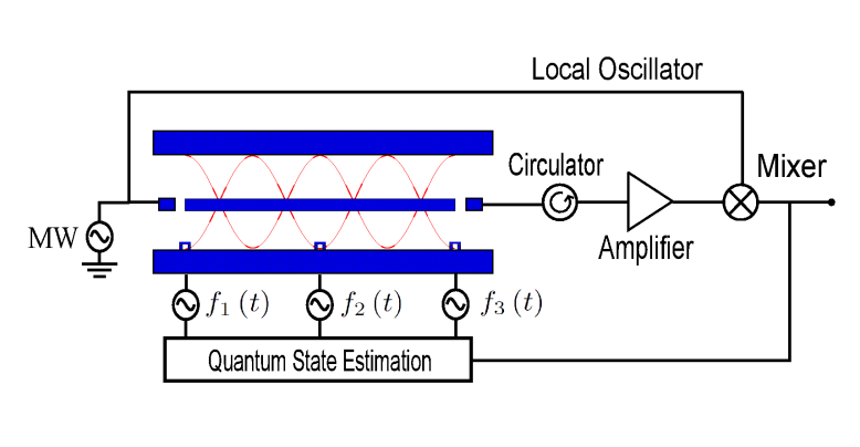
We consider a circuit QED setup in which three Cooper pair boxes considered as qubits are coupled to a common field of a one-dimensional microwave transmission line resonator (TLR) treated as a cavity (see Fig. 1). The system can be described well by the Tavis-Cummings model Blais et al. (2004); Fink et al. (2009); Liu et al. (2010); Feng et al. (2011); Lalumière et al. (2010); Wu and the Hamiltonian driven by a measurement signal is described by

$$H = \omega_{r}a^{\dagger}a+\epsilon\left(ae^{i\omega_{d}t}+a^{\dagger}e^{-i\omega_{d}t}\right)$$ (1)

$$+\sum_{j}\left[\frac{\Omega_{j}}{2}\sigma_{j}^{z}+g_{j}\left(\sigma_{j}^{-}a^{\dagger}+\sigma_{j}^{+}a\right)\right].$$

Here, the operators $\sigma_{j}^{-}$$\left(\sigma_{j}^{+}\right)$ and $a$$\left(a^{\dagger}\right)$ are respectively the lowering (raising) operators of the $j$th qubit and the microwave inside the cavity, $\Omega_{j}$ is the transition frequency of the $j$th qubit, $\omega_{r}$ is the cavity frequency, $g_{j}$ is the strength of the $j$th qubit interacting with the cavity field, and $\epsilon$ and $\omega_{d}$ are the amplitude and frequency of the measurement drive. In the dispersive regime, where $\left|\Delta_{j}\right|=\left|\Omega_{j}-\omega_{r}\right|\gg g_{j}$, we can eliminate the direct qubit-resonator coupling by using the unitary transformation Blais et al. (2004)

$$U=\exp\left[\sum_{j}\lambda_{j}\left(\sigma_{j}^{+}a-\sigma_{j}^{-}a^{\dagger}\right)\right].$$ (2)

Keeping terms in the Hamiltonian up to second order in the small parameter $\lambda_{j}=g_{j}/\Delta_{j}$ and moving to a frame rotating with the measurement signal frequency $\omega_{d}$ for the cavity field and qubits, we obtain the Hamiltonian Lalumière et al. (2010)

$$H_{\text{eff}} = \left[\delta_{r}+\sum_{j}\chi_{j}\sigma_{j}^{z}\right]a^{\dagger}a+\epsilon\left(a+a^{\dagger}\right)+\sum_{j}\epsilon\lambda_{j}\sigma_{j}^{x}$$ (3)

$$+\sum_{j}\frac{\tilde{\Omega}_{j}}{2}\sigma_{j}^{z}+\sum_{j>i}J_{ij}^{q}\left(\sigma_{i}^{-}\sigma_{j}^{+}+\sigma_{i}^{+}\sigma_{j}^{-}\right).$$

Here, the detuning frequency between cavity and the measurement drive $\delta_{r}=\omega_{r}-\omega_{d}$, the dispersive coupling strength $\chi_{j}=g_{j}\lambda_{j}=g_{j}^{2}/\Delta_{j}$, the dispersive-shifted qubit frequency $\tilde{\Omega}_{j}=\Omega_{j}-\omega_{d}+\chi_{j}$, and the strength of qubit-qubit interaction mediated by the cavity field $J_{ij}^{q}=g_{i}g_{j}\left[\left(1/\Delta_{i}\right)+\left(1/\Delta_{j}\right)\right]/2$. One can see that in this dispersive limit, the qubit-resonator interaction induces a qubit-state-dependent shift on the resonator frequency. If we set $\delta_{r}=\omega_{r}-\omega_{d}=0$, i.e., the driving frequency to be in resonance with the cavity frequency, the measurement of the resonator frequency shift can be translated into the measurement of the phase shift between the incident and transmitted microwave drives. Thus the information about the qubit state can be inferred from the homodyne signal coming from the transmitted microwave through the cavity or TLR. The optimal signal to noise ratio for single-qubit dispersive readout is achieved for $2\chi=\kappa$ Gambetta et al. (2008) while it is a little bit involved when multi-qubit joint measurement is considered [see discussions related to Eqs. (17) and (21) and to the red dashed curve in Fig. 5(a)].

The evolution equation for the density matrix of the qubit and cavity system conditioned on the continuous homodyne detection in the joint rotating frame can be written as Wiseman and Milburn (1993); Wiseman09

$$\dot{\rho}_{c} = -\imath\left[H_{\text{eff}},\rho_{c}\right]+\sum_{j}\gamma_{j}\mathcal{D}\left[\sigma_{j}^{-}\right]\rho_{c}$$ (4)

$$+\kappa\mathcal{D}\left[a\right]\rho_{c}+\sqrt{\kappa\eta}\mathcal{H}[ae^{-i\phi}]\rho_{c}\xi(t),$$

where the effect of the baths on the system describing the qubit and cavity decays is denoted by the decoherence superoperator terms given in the Lindblad form

$$\mathcal{D}\left[c\right]\rho=c\rho c^{\dagger}-\frac{1}{2}\left(c^{\dagger}c\rho+\rho c^{\dagger}c\right),$$ (5)

and $\kappa$ and $\gamma_{i}$ are respectively the cavity and individual qubit decay rates. The last term in the conditional master equation (4) is the homodyne measurement unraveling term that describes the back action and stochastic nature of the quantum measurements, $0\leq\eta\leq 1$ is the measurement efficiency ($\eta=1$ corresponds to a perfect detector or efficient measurement, and $\eta<1$ represents the fraction of detections which are actually registered by the detectors), $\phi$ is the phase of the local oscillator that is mixed with the transmitted microwave in the homodyne measurement, and the measurement superoperator

$$\mathcal{H}\left[c\right]\rho=c\rho+\rho c^{\dagger}-\left\langle c+c^{\dagger}\right\rangle\rho,$$ (6)

where $\left\langle c\right\rangle=\text{tr}\left(\rho c\right)$ means the quantum average of the operator $c$. The stochastic nature of the random measurement outcomes is characterized by $\xi(t)$, a Gaussian white noise with the ensemble average properties of $E[\xi(t)]=0$, $E[\xi(t)\xi(t^{\prime})]=\delta(t-t^{\prime})$, where $E[\cdots]$ denotes an ensemble average over different realizations of the noise. The use of a Gaussian white noise term here assumes that the local oscillator has no more noise than a coherent state, a good assumption at microwave frequencies. The measured homodyne current (in units of frequency) is proportional to

$$I(t)=\kappa\eta\langle a\,e^{-i\phi}+a^{\dagger}\,e^{i\phi}\rangle+\sqrt{k\eta}\xi(t).$$ (7)

Although Eq. (4) can be used to study the conditional dynamics and measurement backaction, it provides little direct insight about how the evolution of the qubits depends on the continuous measurement outcomes. However, if the cavity field can be traced out and an effective (stochastic) master equation for the qubit degrees of freedom only can be obtained, more intuition and understanding to the qubit dynamics of the continuous quantum measurement process can be gained and thus help facilitate the successful development and design of further manipulation and control strategies for the qubit system, e.g., the quantum feedback control strategy presented later in this article.

To obtain the effective stochastic master equation for the qubits’ degrees of freedom only, a common method is the so-called adiabatic elimination procedure valid in the limit where the damping of the cavity is much larger than both the dispersive coupling strengths and the qubits’ decay rates, i.e., $\kappa\gg(\chi_{i}$ and $\gamma_{i})$. Here, we go beyond this limit and use a polaron-type transformation Gambetta et al. (2008); Lalumière et al. (2010) to trace out the cavity field. We will compare these two approaches in Sec. IV. The polaron-type approach assumes only that the state of the qubits varies slowly within the measurement time during which the cavity field evolves to a steady coherent state depending on the qubit state. This assumption can be justified if the cavity field decay rate is much faster than the qubit decay rate $\kappa\gg 2\gamma_{j}$. In this case, the unconditional master equation, i.e., Eq. (4) averaged over the white noise process, indicates that a coherent state remains a coherent state with the amplitude $\alpha_{x}$ of the cavity coherent state $|\alpha_{x}\rangle$ at $\delta_{r}=\omega_{r}-\omega_{d}=0$ satisfying

$$\dot{\alpha}_{x}=-\imath\chi_{x}\alpha_{x}-\imath\epsilon-\frac{\kappa}{2}\alpha_{x}$$ (8)

when the qubits are in a basis state $\left|x\right\rangle=\left|ijk\right\rangle$, where $i,j,k\in\left\{0,1\right\}$, $\left|0\right\rangle$ and $\left|1\right\rangle$ represent respectively the ground and excited states of a single qubit, and $\chi_{x}=\left\langle x\right|\sum_{j}\chi_{j}\sigma_{j}^{z}\left|x\right\rangle$. Then the elimination of the cavity (TLR) degrees of freedom is carried out by going to a frame defined by the transformation Gambetta et al. (2008); Lalumière et al. (2010)

$$\mathbf{P}\left(t\right)=\sum_{x}\Pi_{x}D\left[\alpha_{x}\left(t\right)\right]$$ (9)

with $D\left[\alpha\right]$ the displacement operator of the TLR,

$$D\left[\alpha\right]=\exp\left[\alpha a^{\dagger}-\alpha^{*}a\right],$$ (10)

and $\Pi_{x}=\left|x\right\rangle\left\langle x\right|$ are projection operators onto the respective basis (logical) states of the three-qubit Hilbert space. In this transformed reference frame, the cavity field is displaced to start from a vacuum state with zero photon, i.e., $D\left[\alpha_{x}\right]|0\rangle_{TLR}=|\alpha_{x}\rangle_{TLR}$. For simplicity, we take $\Omega_{1}=\Omega_{2}=\Omega_{3}=\Omega$ and $g_{1}=g_{2}=g_{3}=g$. This implies that we assume three identical qubits with one wavelength separation apart in the TLR cavity (see Fig. 1). This assumption also helps generate the $|W^{-}\rangle$ state by continuous measurements as the $|W^{-}\rangle$ state in this case is a simultaneous eigenstate of the system Hamiltonian (i.e., when without consideration of the qubits’ decay) and the homodyne measurement operator [see Eq. (21) and further discussion below it]. Then following the calculations in Refs. Gambetta et al., 2008; Lalumière et al., 2010, we obtain an effective master equation for the qubits’ degrees of freedom alone conditioned on continuous homodyne detection as Gambetta et al. (2008); Tornberg and Johansson (2010); Lalumière et al. (2010)

$$d\rho_{c}\left(t\right)/dt = \mathcal{L}\rho_{c}\left(t\right)+\sqrt{\kappa\eta}\mathcal{H}\left[c_{\phi}\right]\rho_{c}\left(t\right)\xi\left(t\right)-\imath\sqrt{\kappa\eta}\left[c_{\phi-\pi/2},\rho_{c}\left(t\right)\right]\xi\left(t\right),$$ (11)

where $\mathcal{L}\rho_{c}$ is given by

$$\mathcal{L}\rho_{c} = -\imath\left[\sum_{j}\frac{\chi}{2}\sigma_{j}^{z}+\sum_{j}\epsilon\lambda(\sigma_{j}^{+}e^{i\Delta t}+\sigma_{j}^{-}e^{-i\Delta t})+\sum_{j>i}\chi\left(\sigma_{i}^{-}\sigma_{j}^{+}+\sigma_{i}^{+}\sigma_{j}^{-}\right),\rho_{c}\right]$$ (12)

$$+\sum_{j}\gamma_{j}\mathcal{D}\left[\sigma_{j}^{-}\right]\rho_{c}+\kappa\mathcal{D}\left[\sum_{j}\lambda\sigma_{j}^{-}\right]\rho_{c}+\sum_{xy}\left(\Gamma_{d}^{xy}-\imath A_{c}^{xy}\right)\Pi_{x}\rho_{c}\Pi_{y}.$$

In writing Eq.(12), we have transformed to a frame rotating with the qubits’ transition frequency $\Omega$. This is also a suitable frame for applying an additional microwave drive with a frequency in resonance with the qubits’ transition frequency in order to coherently control the qubits as discussed in the context of quantum feedback control in the next section. As a result, the $\sigma_{x}$ term in Eq. (3) now acquires time-dependent oscillating factors with frequency $\Omega-\omega_{d}=\Delta$ (as we have set $\omega_{d}=\omega_{r}$) in the commutator of the first term in Eq. (12). The third term in Eq. (12) represents the Purcell effect at the damping rate $\kappa\lambda^{2}$ which can be reduced by operating the qubits in the dispersive regime Boissonneault et al. (2009); Houck et al. (2008); Filipp et al. (2011), while the fourth term contains both the measurement-induced dephasing $\left(\Gamma_{d}^{xy}\right)$ and the ac Stark shift $\left(A_{c}^{xy}\right)$ given by

$$\Gamma_{d}^{xy} = \left(\chi_{x}-\chi_{y}\right)\text{Im}\left[\alpha_{x}\alpha_{y}^{*}\right],$$ (13)

$$A_{c}^{xy} = \left(\chi_{x}-\chi_{y}\right)\text{Re}\left[\alpha_{x}\alpha_{y}^{*}\right].$$ (14)

The last two terms of Eq. (11) come from the last term of the conditional master equation (4) in the displaced polaron-type frame, in which the cavity field is transformed into

$$a\,e^{-i\phi}\to\sum_{x}\Pi_{x}\alpha_{x}e^{-i\phi}=c_{\phi}-ic_{\phi-\pi/2}.$$ (15)

The measured homodyne current from Eq. (7) becomes

$$I_{c}\left(t\right)=\kappa\eta\left\langle c_{\phi}+c_{\phi}^{\dagger}\right\rangle_{c}\left(t\right)+\sqrt{\kappa\eta}\xi\left(t\right).$$ (16)

Here the joint measurement operator $c_{\phi}$ is given by Gambetta et al. (2008); Tornberg and Johansson (2010); Lalumière et al. (2010)

$$c_{\phi}=\frac{1}{2}\sum_{i,j,k=0}^{1}\sqrt{\Gamma_{ijk}\left(\phi\right)}\left(\sigma^{z}_{1}\right)^{i}\left(\sigma^{z}_{2}\right)^{j}\left(\sigma^{z}_{3}\right)^{k},$$ (17)

where

$$\Gamma_{ijk}\left(\phi\right)=\left|\beta_{ijk}\right|^{2}\cos^{2}\left(\phi-\theta_{\beta_{ijk}}\right),$$ (18)

$$\beta_{ijk}=\frac{1}{4}\sum_{l,m,n=0}^{1}\left(-1\right)^{\vec{a}\cdot\vec{b}}\alpha_{lmn},$$ (19)

where the vectors are $\vec{a}=\left(i,j,k\right)$ and $\vec{b}=\left(1-l,1-m,1-n\right)$, $\theta_{\beta}=\arg\left(\beta\right)$, and $\kappa\eta\Gamma_{ijk}\left(\phi\right)$ is the measurement rate for the polarization of $\left(\sigma^{z}_{1}\right)^{i}\left(\sigma^{z}_{2}\right)^{j}\left(\sigma^{z}_{3}\right)^{k}$. Note that the conditional stochastic master equation (11) after being averaged over all possible measurement records reduces to the unconditional, deterministic master equation, i.e., Eq. (11) but without its last two unraveling noise terms.

The outcomes of the homodyne current (16) depend on the choice of the local oscillator phase $\phi$. We would like to generate the entanglement state $|W^{-}\rangle$ by quantum measurement. Thus we choose the phase to be $\phi=0$ such that $|W^{-}\rangle$ state is one of the eigenstates of the measurement operator Bishop2009 ; Chow et al. (2010); Spilla2012 ; Feng et al. (2011)

$$c_{0} = \frac{3\sqrt{\Gamma_{0}}-\sqrt{\Gamma_{1}}}{2}\left(\Pi_{111}-\Pi_{000}\right)$$ (20)

$$+\frac{\sqrt{\Gamma_{0}}+\sqrt{\Gamma_{1}}}{2}\left(\Pi_{011}+\Pi_{101}+\Pi_{110}-\Pi_{100}-\Pi_{010}-\Pi_{001}\right)$$

$$= \frac{\sqrt{\Gamma_{0}}}{2}\left(\sigma_{1}^{z}+\sigma_{2}^{z}+\sigma_{3}^{z}\right)-\frac{\sqrt{\Gamma_{1}}}{2}\sigma_{1}^{z}\sigma_{2}^{z}\sigma_{3}^{z},$$ (21)

where

$$\sqrt{\Gamma_{0}} = \sqrt{\Gamma_{100}}=\sqrt{\Gamma_{010}}=\sqrt{\Gamma_{001}}$$ (22)

$$= \frac{1}{4}(\alpha_{111}-\alpha_{000}+\alpha_{110}-\alpha_{001}),$$

and

$$\sqrt{\Gamma_{1}} = \sqrt{\Gamma_{111}}$$ (23)

$$= \frac{1}{4}(\alpha_{000}-\alpha_{111}+3\alpha_{001}-3\alpha_{110}).$$

In this case, there are four measurement outcomes of $\langle c_{0}+c_{0}^{\dagger}\rangle$: $3\sqrt{\Gamma_{0}}-\sqrt{\Gamma_{1}}$, $\sqrt{\Gamma_{0}}+\sqrt{\Gamma_{1}}$, $-\sqrt{\Gamma_{0}}-\sqrt{\Gamma_{1}}$, and $-3\sqrt{\Gamma_{0}}+\sqrt{\Gamma_{1}}$ which correspond respectively to the all-qubit excited state $\left|111\right\rangle$, the two-qubit excited states $\left\{\left|110\right\rangle,\left|101\right\rangle,\left|011\right\rangle\right\}$, the single-qubit excited states $\left\{\left|001\right\rangle,\left|010\right\rangle,\left|100\right\rangle\right\}$, and the ground state $\left|000\right\rangle$. One can see from Eq. (15) and the last two terms of Eq. (11) that in addition to the measurement operator $c_{0}$ providing the qubit state information, performing the homodyne measurement at $\phi=0$ also produces a stochastic phase represented by the term associated with

$$c_{-\pi/2} = \frac{3\sqrt{\Gamma_{2}}}{2}\left(\Pi_{111}+\Pi_{000}\right)$$ (24)

$$-\frac{\sqrt{\Gamma_{2}}}{2}\left(\Pi_{011}+\Pi_{101}+\Pi_{110}+\Pi_{100}+\Pi_{010}+\Pi_{001}\right)$$

$$= \frac{\sqrt{\Gamma_{2}}}{2}\left(\sigma_{1}^{z}\sigma_{2}^{z}+\sigma_{2}^{z}\sigma_{3}^{z}+\sigma_{1}^{z}\sigma_{3}^{z}\right),$$ (25)

where

$$\sqrt{\Gamma_{2}} = \sqrt{\Gamma_{011}}=\sqrt{\Gamma_{101}}=\sqrt{\Gamma_{110}}$$ (26)

$$= \frac{i}{4}(\alpha_{111}+\alpha_{000}-\alpha_{110}-\alpha_{001}).$$

Note that $c_{-\pi/2}$ generates different relative phase kicks only between two groups of states, i.e., between the group of $\left\{\left|111\right\rangle,\left|000\right\rangle\right\}$ and the group of $\left\{\left|110\right\rangle,\left|101\right\rangle,\left|011\right\rangle,\left|001\right\rangle,\left|010\right\rangle,\left|100\right\rangle\right\}$. In other words, no relative random phase kick between the constituent basis states of the $|W^{-}\rangle$ state (thus no additional unwanted dephasing between them) also helps generate and stabilize the target $|W^{-}\rangle$ state.

When the coherent state amplitudes are steady, the rates $\kappa\Gamma_{0}$, $\kappa\Gamma_{1}$ and $\kappa\Gamma_{2}$ become

$$\sqrt{\kappa\Gamma_{0}} = \sqrt{\Gamma_{\rm m}}\left[\frac{1+12\left(\chi/\kappa\right)^{2}}{1+40\left(\chi/\kappa\right)^{2}+144\left(\chi/\kappa\right)^{4}}\right],$$ (27)

$$\sqrt{\kappa\Gamma_{1}} = \sqrt{\Gamma_{\rm m}}\left[\frac{24\left(\chi/\kappa\right)^{2}}{1+40\left(\chi/\kappa\right)^{2}+144\left(\chi/\kappa\right)^{4}}\right],$$ (28)

$$\sqrt{\kappa\Gamma_{2}} = \sqrt{\Gamma_{\rm m}}\left[\frac{-4\left(\chi/\kappa\right)}{1+40\left(\chi/\kappa\right)^{2}+144\left(\chi/\kappa\right)^{4}}\right],$$ (29)

where $\Gamma_{\rm m}=64\epsilon^{2}\chi^{2}/\kappa^{3}$ is the effective measurement rate obtained from the adiabatic elimination method Sarovar05 ; Liu et al. (2010). In general, the measurement rate is related to the decoherence rate as the decrease in the off-diagonal element is associated with the gradual projection onto one of the corresponding measurement eigenstates. For example, in the steady state , the measurement rate $\Gamma_{\rm m}$ for efficiency $\eta=1$ is equal to twice of the decoherence rate, i.e., $\Gamma_{\rm m}=2\Gamma_{\rm e}$, for the case by the adiabatic elimination method [see Eq.(35)] Liu et al. (2010). Similarly, there is a relationship between the measurement rates defined through Eq. (21) and the corresponding decoherence rates in Eq. (13). We may define for efficiency $\eta=1$ the ratio between them as

$$R_{x,y}\equiv\frac{\kappa\left|\alpha_{x}-\alpha_{y}\right|^{2}}{\left(\chi_{x}-\chi_{y}\right)\text{Im}\left[\alpha_{x}\alpha^{*}_{y}\right]},$$ (30)

where the numerator, $\kappa\left|\alpha_{x}-\alpha_{y}\right|^{2}$, is the measurement rate to distinguish between two eigenstates $|x\rangle$ and $|y\rangle$ of the measurement operator $c_{0}$ (also proportional to the separation between two measurement outcomes corresponding to the states $|x\rangle$ and $|y\rangle$), and the denominator is the measurement-induced dephasing in Eq. (13). When the coherent amplitudes have reached steady state, it can be shown that

$$R_{000,111}=R_{100,011}=R_{010,101}=R_{001,110}=2.$$ (31)

In other words, the measurement rates to distinguish between the states $\left|111\right\rangle\leftrightarrow\left|000\right\rangle$, $\left|011\right\rangle\leftrightarrow\left|100\right\rangle$, $\left|101\right\rangle\leftrightarrow\left|010\right\rangle$, and $\left|110\right\rangle\leftrightarrow\left|001\right\rangle$ are twice of their corresponding measurement-induced dephasing rates.

We wish to apply the measurement-guided quantum feedback control to generate and stabilize the $|W^{-}\rangle$ state, thus distinct values of measurement current, which reveal quickly the information of corresponding qubit states are favorable. The separations between adjacent measurement outcomes are $2\sqrt{\Gamma_{0}}\pm 2\sqrt{\Gamma_{1}}$ that depend on the value of $\chi/\kappa$. Generally, larger separation between measurement outcomes implies quicker corresponding measurement eigenstate readout. Let us focus on the smaller separation of $2\sqrt{\Gamma_{0}}-2\sqrt{\Gamma_{1}}$ between the measurement outcome of the ground state and that of the $|W^{-}\rangle$ state (or the single-qubit excited states). When the ratio $\chi/\kappa$ is decreased from $0$ to $-1$ , the separation between the outcomes of the ground state and the single-qubit excited state [see the red-dashed curve in Fig. 5(a)] increases initially, and then reaches a local maximum around $\chi/\kappa=-0.11$. It then vanishes around $\chi/\kappa=-0.29$ and later reaches another local maximum around $\chi/\kappa=-0.77$. However, a larger $\chi$ value leads to a larger damping rate, $\kappa\lambda^{2}=\kappa\chi^{2}/g^{2}$, of the Purcell effect which deteriorates the average fidelity to generate and stabilize the $|W^{-}\rangle$ state. As a result, the fidelity at $\chi=-0.77\kappa$ is expected to be smaller than that at $\chi=-0.11\kappa$. We will show later that the average fidelity at $\chi=-0.77\kappa$ is also smaller than that at, say, $\chi=-0.5\kappa$ even though its measurement outcome separation is larger [see Fig. 55 and the discussion related to it in Sec. III.2]. Thus for the simulations presented in this article, the dispersive coupling strength is chosen to be $\chi=-0.11\kappa$ and/or $\chi=-0.50\kappa$. These are readily accessible parameter values Gambetta et al. (2006); Schuster07 ; Fink08 ; Bishop09 .

Figure 2: (Color online) Measured homodyne currents $\langle c_{0}+c^{\dagger}_{0}\rangle_{c}$ ($1000$ realizations that yield roughly the same steady outcome values are grouped and averaged) for an initial cavity state in a vacuum state and an initial qubits’ state in the separable state $\left|\psi_{i}\right\rangle$ of Eq. (32) with the qubits’ decay rates $\gamma_{j}=0$. The four measurement outcomes in solid lines are for the case of polaron-type transformation and they correspond to the qubits collapsing respectively onto states $\left|111\right\rangle$, $\left|W^{+}\right\rangle$, $\left|W^{-}\right\rangle$, and $\left|000\right\rangle$ from the top to the bottom, while the measurement outcomes in dashed lines corresponds to the case of adiabatic elimination. The parameters used are $\epsilon=2\kappa$, $\chi=-0.11\kappa$, $g=10\kappa$, $\eta=1$, and $\gamma_{j}=0$.

Suppose we start to evolve the conditional master equation (11) with an initial state of the cavity in a vacuum state and the qubits in a separable state

$$\left|\psi_{i}\right\rangle=\frac{1}{\sqrt{2}}\left(\left|0\right\rangle+\left|1\right\rangle\right)_{1}\otimes\frac{1}{\sqrt{2}}\left(\left|0\right\rangle+\left|1\right\rangle\right)_{2}\otimes\frac{1}{\sqrt{2}}\left(\left|0\right\rangle+\left|1\right\rangle\right)_{3}.$$ (32)

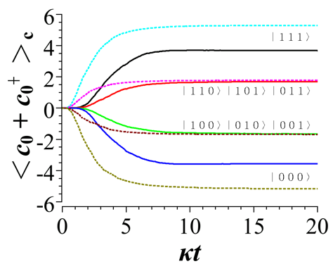
Ideally, it is expected that the qubits under continuous measurements will collapse gradually onto one of the eigenstates of the joint-qubit measurement operator $c_{0}$ stochastically in each individual realization. Indeed, by ignoring the decay rates of the qubits, i.e., by setting $\gamma_{j}=0$, the initial qubit state $\left|\psi_{i}\right\rangle$ of Eq. (32) will collapse onto the states $\left|111\right\rangle$ and $\left|000\right\rangle$ with probability $0.125$ each, and onto the states $\left|W^{+}\right\rangle=(|110\rangle+|101\rangle+|011\rangle)/\sqrt{3}$ and $\left|W^{-}\right\rangle=(|100\rangle+|010\rangle+|001\rangle)/\sqrt{3}$ with probability $0.375$ each. This is shown in Fig. 2 where the averaged measured currents $\langle c_{0}+c^{\dagger}_{0}\rangle_{c}$ obtained by categorizing and averaging $1000$ realizations that yield roughly the same steady outcome values [as implied by Eq. (32)] are presented. One can see that after the time of about $5/\kappa$, the cavity field has evolved from the initial vacuum state to correspondingly distinguishable coherent states and four distinct measurement outcomes (solid lines in Fig. 2) are observed. The measurement outcomes maintaining at certain values for a considerably long time indicate that the qubits have collapsed onto and stayed in the corresponding states of $\left|111\right\rangle$, $\left|W^{+}\right\rangle$, $\left|W^{-}\right\rangle$ and $\left|000\right\rangle$. However, this scheme of producing entangled $|W^{-}\rangle$ or $\left|W^{+}\right\rangle$ states by measurement only is probabilistic, and in the presence of qubit relaxation, the probabilistically generated entangled state will jump into other states.

III Entanglement creation and stabilization by quantum feedback control

III.1 Quantum feedback control strategy

To generate the $|W^{-}\rangle$ state deterministically and stabilize it against the influence of the environments, we employ the adaptive quantum feedback control technique based on quantum state estimation. The conditional stochastic master equation with this kind of the feedback control scheme becomes Sarovar05 ; Liu et al. (2010); Ahn et al. (2002)

$$\dot{\rho}_{c}\left(t\right) = \mathcal{L}\rho_{c}\left(t\right)+\sqrt{\kappa}\mathcal{H}\left[c_{0}\right]\rho_{c}\left(t\right)\xi\left(t\right)-\imath\sqrt{\kappa}\left[c_{-\pi/2},\rho_{c}\left(t\right)\right]\xi\left(t\right)$$ (33)

$$-i[H_{\rm fb}(t),\rho_{c}(t)].$$

Here $H_{\rm fb}\left(t\right)$ is the feedback control Hamiltonian with control parameters designed from an estimation of $\rho_{c}\left(t\right)$. The advantage of the quantum state estimation scheme is that the feedback control can be designed from an optimal control method to ensure the qubit system passing through the more efficient trajectory by optimizing the targeted objective or minimizing the cost function. We choose the objective function to be the fidelity $F_{c}={\rm Tr}\left[\rho_{c}(t)\rho_{W^{-}}\right]$, where $\rho_{W^{-}}=|W^{-}\rangle\langle W^{-}|$, and choose the feedback control Hamiltonian to be $H_{\rm fb}=f_{1}\sigma^{x}_{1}+f_{2}\sigma^{x}_{2}+f_{3}\sigma^{x}_{3}$, i.e., only single qubit rotations. The strategy Ahn et al. (2002) to determine the feedback strengths $f_{j}$ at each point in time is chosen optimally by maximizing the fidelity $F_{c}={\rm Tr}\left[\rho_{c}(t)\rho_{W^{-}}\right]$. By considering the dynamics of the feedback Hamiltonian only, $\dot{\rho}_{c}(t)=-i[H_{\rm fb},\rho_{c}(t)]$, the time evolution of the fidelity is

$$\frac{dF_{c}(t)}{dt} = {\rm Tr}[\dot{\rho}_{c}(t)\rho_{W^{-}}]=\left\langle-\imath\left[\rho_{W^{-}},H_{\rm fb}\right]\right\rangle_{c}$$ (34)

$$= f_{1}\left\langle-\imath\left[\rho_{W^{-}},\sigma_{1}^{x}\right]\right\rangle_{c}+f_{2}\left\langle-\imath\left[\rho_{W^{-}},\sigma_{2}^{x}\right]\right\rangle_{c}+f_{3}\left\langle-\imath\left[\rho_{W^{-}},\sigma_{3}^{x}\right]\right\rangle_{c}.$$

To maximize the fidelity, i.e., to make $[{dF_{c}(t)}/{dt}]$ positive and maximal, the optimal feedback coefficients to kick the qubit system back to the desired state $\rho_{W^{-}}=|W^{-}\rangle\langle W^{-}|$ are determined by $f_{j}=f{\rm sgn}\left(\langle-\imath\left[\rho_{W^{-}},\sigma_{j}^{x}\right]\rangle_{c}\right)$, where sgn($y$) denotes the sign function that extracts the sign of a real number $y$, and $f$ is the maximum feedback strength that can be applied. This is a bang-bang feedback control scheme, meaning that the feedback strengths are always at the maximum or minimum values Ahn et al. (2002).

III.2 Entanglement Creation and Stabilization

Figure 3: (Color online) Time evolutions of the average fidelity $F$ of $\left|W^{-}\right\rangle$ state (over 1000 realizations or trajectories) as a function of time for different initial states of $\left|000\right\rangle$, $\left|W^{-}\right\rangle$, $\left|W^{+}\right\rangle$, $\left|000\right\rangle$ and $\left|\psi_{i}\right\rangle$. The parameters used are $f=2\kappa$, $\epsilon=2\kappa$, $\chi=-0.11\kappa$, $g=10\kappa$, $\eta=1$, and $\gamma_{j}=\gamma=4\times 10^{-3}\kappa$.

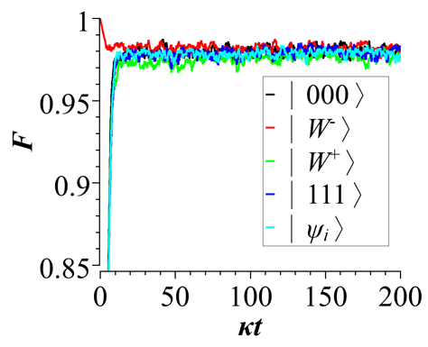
Considering qubits’ decay rates $\gamma_{j}=\gamma=\kappa/250$ as in Ref. Lalumière et al. (2010), we demonstrate in Fig. 3 that the entangled $\left|W^{-}\right\rangle$ state can be generated and stabilized with high average fidelity $F\approx 0.98$ for various initial qubits’ states by our feedback control strategy with a moderate feedback strength of $f=2\kappa$. The average fidelity $F$ is obtained by averaging $F_{c}$ over $1000$ realizations or trajectories. The various initial states are $|000\rangle$, $|W^{-}\rangle$, $|W^{+}\rangle$, $|111\rangle$, eigenstates of the joint measurement operator $c_{0}$, and the separable state $|\psi_{i}\rangle$ of Eq. (21). They all reach the average fidelity of about $0.98$ in a time scale of about a few $1/\kappa$, in about the same time scale for the cavity field to evolve into distinguishable coherent states (without feedback control) in Fig. 2. Other parameters used in Fig. 3 are the coupling strength $g=10\kappa$, and the dispersive coupling strength $\chi=-0.11\kappa$.

Figure 4: (Color online) (a) Time evolutions of the average fidelity $F$ of the $\left|W^{-}\right\rangle$ state (over 1000 trajectories) generated from the ground state $\left|000\right\rangle$ for different qubits’ decay rates of $\gamma_{j}=\gamma$ being $4\times 10^{-3}\kappa$, $1\times 10^{-2}\kappa$, $2\times 10^{-2}\kappa$, and $4\times 10^{-2}\kappa$ (solid lines from top to bottom). The brown-dashed line is the ensemble average fidelity without the application of feedback control for an initial qubits’ state being in $\left|W^{-}\right\rangle$. (b) A typical single trajectory of the estimated current $\langle c_{0}+c^{\dagger}_{0}\rangle_{c}$ for the qubits’ decay rates of $\gamma_{j}=\gamma=4\times 10^{-3}\kappa$. The qubits’ system is stabilized in the $|W^{-}\rangle$ state with $\langle c_{0}+c^{\dagger}_{0}\rangle_{c}=-1.68$ during the continuous feedback control process (in solid line), while it makes a sudden jump to the ground state $\left|000\right\rangle$ with $\langle c_{0}+c^{\dagger}_{0}\rangle_{c}=-3.68$ without the application of feedback control (in dashed line. Other parameters used are the same as those in Fig. 3.

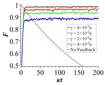
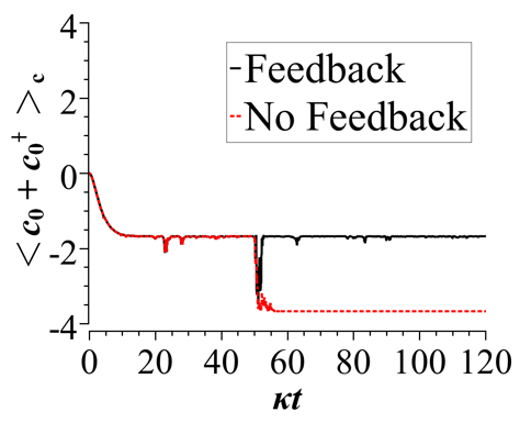
Figure 4(a) shows the time evolutions of the average fidelity of the $\left|W^{-}\right\rangle$ state for different qubit decay rates. The brown-dashed line is the ensemble average (unconditional) result of the qubit system evolving from the $\left|W^{-}\right\rangle$ state without feedback control for the qubit decay rates of $\gamma_{j}=\gamma=4\times 10^{-3}\kappa$. The fidelity without feedback control deteriorates about linearly with time. This can be understood from a typical measured current record in a single realization of the experiment as shown in Fig. 4(b). The qubits initially in the $\left|W^{-}\right\rangle$ state corresponding to the result of $\langle c_{0}+c^{\dagger}_{0}\rangle_{c}=-1.68$ for the parameters chosen here have probability $\gamma dt$ to make a sudden jump into the ground state $\left|000\right\rangle$ corresponding to $\langle c_{0}+c^{\dagger}_{0}\rangle_{c}=-3.68$ in the time interval $\left[t,t+dt\right]$. If there is no feedback control, the qubit after the sudden jump will then stay in the ground state as indicated by the red-dashed curve in Fig. 4(b). In contrast, even when the initial qubit state is the ground state $\left|000\right\rangle$, the qubit with feedback control will be driven to the $\left|W^{-}\right\rangle$ state and be stabilized for a sufficient long time. This is also shown in Fig. 4(a) in which the ensemble averaged fidelities with application of feedback control (even when the decay rate of the qubits is $\gamma_{j}=\gamma=\kappa/25=4\times 10^{-2}\kappa$) are stabilized with values above that of the brown-dashed line (with $\gamma_{j}=\gamma=\kappa/25$) when time $\kappa t>50$.

Figure 5: (Color online) Dependence of the average fidelity $F$ of the $\left|W^{-}\right\rangle$ state at $\kappa t=350$ on 5 the dispersive coupling strength $\chi$, 5 the driving amplitude $\epsilon$, 5 the feedback strength $f$ and 5 the measurement efficiency $\eta$. The decay rate of the qubits is fixed at $\gamma_{j}=\gamma=4\times 10^{-3}\kappa$ and the initial qubit state is the ground state $\left|000\right\rangle$. The red-dashed curve in 5 is the separation between the measurement outcomes of the ground state and the $\left|W^{-}\right\rangle$ state (or the single-qubit excited state) with its vertical axis label shown on the right.

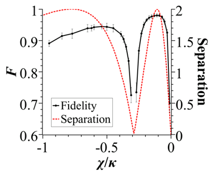
We discuss in the following the dependence of the average fidelity on the dispersive coupling strength $\chi$, the probe beam amplitude $\epsilon$, the feedback strength $f$, and the measurement efficiency $\eta$. The black-circle solid line in Fig. 55 is the average fidelity $F$ versus the dispersive coupling strength $\chi$ for the probe field $\epsilon=2\kappa$, the feedback strength $f=2\kappa$, and the decay rate of the qubits $\gamma_{j}=\gamma=4\times 10^{-3}\kappa$. The dependence of the fidelity on $\chi$ is similar to the red-dashed curve which represents the separation between the measurement output signal $\langle c_{0}+c^{\dagger}_{0}\rangle_{c}$ that corresponds to the qubits’ state being in $\left|W^{-}\right\rangle$ and the output signal that corresponds to the qubits’ state of $\left|000\right\rangle$. This is because larger separation means better state distinguishibility and thus helps the conditional qubits’ state estimation in the quantum feedback control scheme. One can observe that $\left|W^{-}\right\rangle$ and $\left|000\right\rangle$ become indistinguishable from the measurement current around the point $\chi\approx-0.29\kappa$, and thus the fidelity drops sharply around there as well. One can also notice from Fig. 55 that the separation reaches maximum values at $\chi=-0.11\kappa$ and $\chi=-0.77\kappa$, but the fidelity is higher at $\chi=-0.11\kappa$. This is because the collective damping rate $\kappa\lambda^{2}=\kappa\chi^{2}/g^{2}$ of the Purcell effect of the third term in Eq. (12) increases with the values of $\chi$. For example, for $g=10\kappa$, the Purcell collective damping rate of $5.93\times 10^{-3}\kappa$ at $\chi=-0.77\kappa$ is larger than the individual qubit decay rate, set to be $\gamma_{j}=\gamma=4\times 10^{-3}\kappa$ here, while the Purcell collective damping rate of $1.21\times 10^{-4}\kappa$ at $\chi=-0.11\kappa$ is much smaller than $\gamma$ and thus does not play an important role. As a result, the average fidelity is lower for the case of a higher $\chi$ value when the corresponding separation of the measurement outcomes is the same. Another observation from Fig. 55 is that the average fidelity does not change with the dispersive coupling strength $\chi$ as sharply as the separation of the measurement outcomes does. When the separation of the measurement outcomes above a certain value (about $1.6$ for the parameters chosen here), the average fidelity does not vary much [see the behaviors of the separation of the measurement outcomes and the average fidelity around $\chi=-0.11\kappa$, where the Purcell effect is not significant as compared to the individual qubits’ decay]. This may also explain why the average fidelity at $\chi=-0.5\kappa$ is larger than that at $\chi=-0.77\kappa$. The Purcell collective damping rate of $2.50\times 10^{-3}\kappa$ at $\chi=-0.5\kappa$, which is smaller than the individual qubit decay rate $\gamma_{j}=\gamma=4\times 10^{-3}\kappa$, is smaller than that of $5.93\times 10^{-3}\kappa$ at $\chi=-0.77\kappa$. Although the separation of the measurement outcomes at $\chi=-0.5\kappa$ is also smaller there, its value is larger than $1.6$. As a result, the average fidelity at $\chi=-0.5\kappa$ is larger than that at $\chi=-0.77\kappa$. We perform most of our simulations choosing $\chi=-0.11\kappa$ and/or $\chi=-0.5\kappa$.

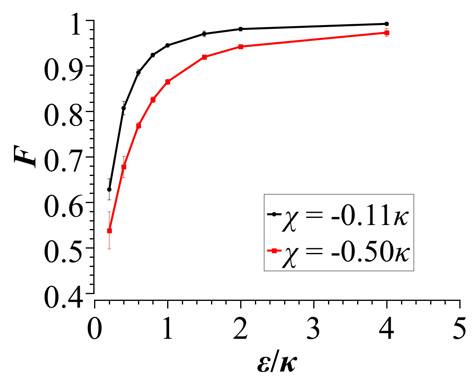
The dependence of average fidelity on the measurement drive amplitude $\epsilon$ is shown in Fig. 55. Since the information gain rates [c.f. Eqs. (27) and (28)] is proportional to $\sqrt{\Gamma_{\rm m}}\propto\epsilon$, the bigger the value $\epsilon$ is, the larger the separation between measurement outcomes is and the quicker the conditional state collapse to one of the joint measurement operator eigenstates is. It is thus expected the average fidelity will also become better as $\epsilon$ increases as shown in Fig. 55. One may be temped to think that the arbitrarily quick readout or arbitrarily high fidelity can be achieved by simply increasing $\epsilon$. But it was pointed out Blais et al. (2004); Gambetta et al. (2006) that the lowest-order dispersive approximation of Hamiltonian Eq. (3) become accurate when the average photon number in the cavity is much smaller than the critical photon number of $n_{\rm crit}=\Delta^{2}/4g^{2}$. The number of photon is proportional to $\epsilon^{2}$. This puts a limit on how large the external drive $\epsilon$ could be for Eq. (3) to hold valid. In addition, note that the time-dependent second term $\sum_{j}\epsilon\lambda(\sigma_{j}^{+}e^{i\Delta t}+\sigma_{j}^{-}e^{-i\Delta t})$ in the first commutator of Eq. (4) also increases with $\epsilon$. This term in the Hamiltonian, in addition to qubit decay channel, will cause the qubits to flip or change their state during the process when the continuous measurement tries to localize the qubits to one of the joint measurement operator eigenstates. However, the value of $\lambda=\chi/g=0.11/10=0.011$ we choose is small and for typical value of $\epsilon$, the coefficient $\epsilon\lambda$ of this term is much smaller than the frequency $\Delta=\Omega-\omega_{d}$ (as we have set $\omega_{d}=\omega_{r}$) of the oscillating factors. Thus the effect of this term to mix different measurement eigenstates is small. We choose $\epsilon=2\kappa$ for most of the simulations presented in this paper although increasing $\epsilon$ further will improve the fidelity a little bit.

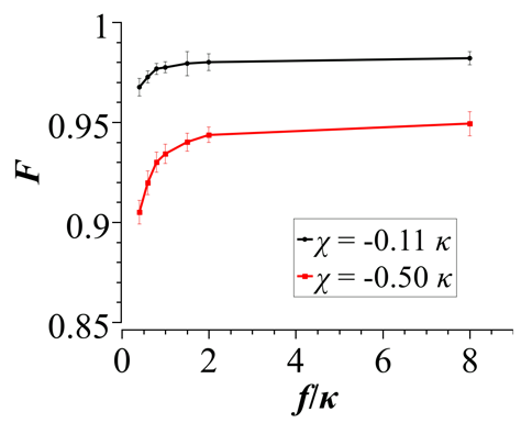
Figure 55 shows that increasing the feedback control strength improves the average fidelity in general. Suppose a measurement outcome indicating deviation from the desired $\left|W^{-}\right\rangle$ state happens, the applied feedback control has to overcome the effect of the localization due to the continuous measurement in order to move the qubits back to the target $\left|W^{-}\right\rangle$ state. When the feedback control strength is smaller, the procedure to produce and stabilize the $\left|W^{-}\right\rangle$ state takes a longer time with a lower fidelity. The qubits’ decay rates in Fig. 55 are chosen to be $\gamma_{j}=\gamma=4\times 10^{-3}\kappa$. When the feedback control strength is $f=2\kappa$, the fidelity reaches the value of $0.98$. Further increase of the feedback control strength, i.e., $f>2\kappa$, does not improve appreciably the fidelity. This indicates that if deviation occurs, the correction of the feedback control at $f=2\kappa$ is fast enough to kick the qubits back to the $\left|W^{-}\right\rangle$ state. We thus choose $f=2\kappa$ for most of our numerical simulations.

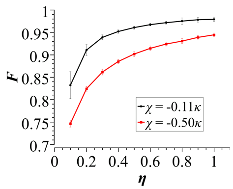
In practice, there exists inefficiency in the measurements which arises when the detectors sometimes miss detection or the measurement microwave photons does not go to the detectors due to lost. However, high measurement efficiency is not very essential for our feedback control scheme. Although the fidelity decreases as the value of the measurement efficiency $\eta$ decreases as shown in Fig. 55, the fidelity is still above $0.9$ for $\eta$ as low as $0.2$ for the case of $\chi=-0.11\kappa$ and qubits’ decay rates $\gamma_{j}=\gamma=4\times 10^{-3}\kappa$. The value of $\eta<1$ implies appearance of an additional non-unraveling dephasing term in the quantum trajectory (stochastic master) equation Tornberg and Johansson (2010). However, this term causes dephasing only among $\left|111\right\rangle$, $\left|W^{+}\right\rangle$, $\left|W^{-}\right\rangle$ and $\left|000\right\rangle$ for the initial qubits’ states chosen in our simulations. As a result, it affects only the detailed dynamics of the qubits but does not destroy or prevent the controlled evolution toward the target entangled state $\left|W^{-}\right\rangle$. Therefore, our feedback control scheme to generate and stabilize the $\left|W^{-}\right\rangle$ state does not require high measurement efficiency and thus can be implemented experimentally with high fidelity with measurement efficiency available in current circuit QED experiments that use parametric amplification before the homodyne detection with an IQ mixer Castellanos-Beltran08 ; Vijay2011 ; Vijay2012 ; Mallet11 . For example, Refs. Vijay2012, ; Mallet11, have achieved an effective quantum efficiency of $\eta=0.4$.

Figure 6: (Color online) Time evolutions of the average fidelity $F$ of the $\left|W^{-}\right\rangle$ state with ($f=2\kappa$) and without ($f=0$) quantum feedback control for three sets of different individual qubits’ decay rates. The initial state for the case with feedback control ($f=2\kappa$) is the ground state $|000\rangle$ while it is the $\left|W^{-}\right\rangle$ state for the case without feedback control ($f=0$). Other parameters used are $\epsilon=2\kappa$, $\chi=-0.11\kappa$, $g=10\kappa$, $\eta=1$, and $\gamma=10^{-2}\kappa$.

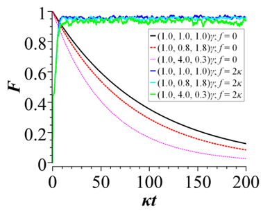
Our feedback control scheme is robust even when the decay rates of the qubits are different. This is shown in Fig. 6 where the time evolutions of the average fidelity of the $\left|W^{-}\right\rangle$ state with and without feedback control for three sets of qubits’ decay rates are shown. The average fidelity is determined roughly by the average decay rate in each set as the behavior of the fidelity in each set is similar to that when the decay rates of the three qubits were equal to the average decay rate. The average fidelities of the $\left|W^{-}\right\rangle$ state generated initially from the ground state $|000\rangle$ with feedback control strength $f=2\kappa$ outperform those evolving from an initial $\left|W^{-}\right\rangle$ state without feedback control ($f=0$) after time $\kappa t\approx 15$.

IV Comparison with adiabatic elimination method

Another commonly used procedure to eliminate the cavity field is the adiabatic elimination method. Both the adiabatic method and the polaron-type transformation method assume that $\kappa\gg\gamma_{i}$, but the adiabatic method employs an additional condition, i.e., to assume that the damping of the cavity is much larger than the dispersive coupling strength, i.e., $\kappa\gg\chi_{i}$. In the limit of $\kappa\gg\chi$, the term $\chi_{x}$ in Eq. (8) is ignored and the TLR cavity field reaches its steady coherent state rapidly with an amplitude equal to $\alpha=-2\imath\epsilon/\kappa$. As a consequence, the coherent state amplitude is assumed to be the same for all the qubits’ basis states. This is in contrast to the case in the polaron-type transformation method where the time-dependent coherent state amplitudes $\alpha_{x}$ shown in Eq. (8) depend on $\chi_{x}$ and thus on the qubits basis states $|x\rangle$. The steady-state information gain rates in the limit of $\kappa\gg\chi$ from Eqs. (27) and (28) become $\sqrt{\kappa\Gamma_{0}}\to\sqrt{\Gamma_{\rm m}}$ and $\Gamma_{1}\to 0$ (note also that $\Gamma_{2}\to 0$). As a result, the measurement operator from Eq. (21) becomes $\sqrt{\Gamma_{e}/\kappa}\sum_{j}\sigma_{j}^{z}$. The effective conditional (stochastic) master equation (11) in the case of adiabatic elimination also reduces to

$$\frac{d\rho_{c}^{\text{e}}\left(t\right)}{dt} = -\imath\left[\sum_{j}[({\chi}/{2})+\chi\left|\alpha\right|^{2}]\sigma_{j}^{z}+\sum_{j}\epsilon\lambda(\sigma_{j}^{+}e^{i\Delta t}+\sigma_{j}^{-}e^{-i\Delta t})+\sum_{j>i}\chi\left(\sigma_{i}^{-}\sigma_{j}^{+}+\sigma_{i}^{+}\sigma_{j}^{-}\right),\rho_{c}^{e}\left(t\right)\right]$$ (35)

$$+\sum_{j}\gamma_{j}\mathcal{D}\left[\sigma_{j}^{-}\right]\rho_{c}^{e}\left(t\right)+\kappa\mathcal{D}\left[\sum_{j}\lambda\sigma_{j}^{-}\right]\rho^{e}_{c}\left(t\right)$$

$$+\frac{\Gamma_{\rm e}}{2}\mathcal{D}\left[\sum_{j}\sigma_{j}^{z}\right]\rho^{e}_{c}\left(t\right)+\frac{\sqrt{\eta\Gamma_{\rm m}}}{2}\mathcal{H}\left[\sum_{j}\sigma_{j}^{z}\right]\rho^{e}_{c}\left(t\right)\xi\left(t\right).$$

Here, the second term in the first commutator term and the fourth term of Eq. (35) are reduced respectively from Eqs. (14) and (13) of Eq. (12). Note again that the measurement rate here is twice of the decoherencee rate, $\Gamma_{\rm m}=2\Gamma_{\rm e}=64\epsilon^{2}\chi^{2}/\kappa^{3}$. One can clearly see that the adiabatic elimination procedure is a special case of polaron-type transformation in the limit of $\kappa\gg\chi$.

The measurement outcomes of the average homodyne currents obtained by categorizing and averaging $1000$ realizations that yield roughly the same steady outcome values for the case of adiabatic elimination are plotted in Fig. 2 to compare with the case of polaron-type transformation with the same parameters. The qubits are initially in the separable state $\left|\psi_{i}\right\rangle$ of Eq. (32) with the qubits’ decay rates set to zero, i.e., $\gamma_{j}=0$, and the cavity state evolves from an initial vacuum state. One can see that the measurement outcomes in dashed lines for the adiabatic elimination case approach to their corresponding steady values more quickly. Moreover, the four measurement outcomes in the adiabatic elimination limit become $3\sqrt{\Gamma_{\rm m}/\kappa}$, $\sqrt{\Gamma_{\rm m}/\kappa}$, $-\sqrt{\Gamma_{\rm m}/\kappa}$, and $-3\sqrt{\Gamma_{\rm m}/\kappa}$; as a result, the steady value corresponding to $\left|111\right\rangle$ ( $\left|000\right\rangle$) is overestimated, i.e., becomes larger (smaller). Thus neglecting the contribution of $\Gamma_{1}\to 0$ in the case of adiabatic elimination for the parameter of $(\chi/\kappa)=-0.11$ used in Fig. 2 is not really valid.

For the adoptive feedback control by state estimation method, it is important to use the correct conditional stochastic master equation to estimate the system state conditioned on the measured current. Otherwise, wrong state estimation information will give rise to bad feedback control result. We have tested numerically that when $|\chi/\kappa|\leq 0.01$ both the adiabatic elimination method and the polaron-type transformation method give the same result for the typical parameters chosen in our simulation in the absent of feedback control. However, when $|\chi/\kappa|>0.02$, discrepancy in conditional qubits’ trajectories starts to emerge. However, Fig. 55 indicates that in the presence of feedback control the average fidelity is below $0.8$ for $\gamma_{j}=\gamma=\kappa/250$ with this value of $|\chi/\kappa|<0.02$. For the value of $(\chi/\kappa)=-0.11$, the fidelity to stabilize the $|W^{-}\rangle$ can be maintained at $0.98$ using the feedback control master equation (33) obtained by the polaron-type transformation method. In other words, in the parameter regime where the adiabatic elimination does not apply, the conditional stochastic master equation (35) can not be used; otherwise the wrong information about the system state will lead to low-fidelity feedback control results. If one would use the conditional master equation (35) obtained by the adiabatic elimination method to perform the feedback control scheme calculation by adding a feedback Hamiltonian commutator term for the case of $(\chi/\kappa)=0.11$, high average fidelity of $0.95$ could be achieved. But this is not correct as the conditional master equation (35) is not really valid when $(\chi/\kappa)=-0.11$. In fact, if we nevertheless use the conditional master equation (35) obtained by the adiabatic elimination method for the state estimation to determine the sign of the feedback strength and then use the polaron-type feedback control master equation (33) (mimicking the real experimental situation) to evolve and calculate the fidelity, the average fidelity is found to be below $0.5$. This is because the signs of the feedback control strength estimated by Eq. (35) obtained by the adiabatic elimination method for the value of $(\chi/\kappa)=-0.11$ are often wrong.

V Conclusion

In conclusion, we have presented a simple and promising quantum feedback control scheme for deterministic generation and stabilization of a three-qubit $|W^{-}\rangle$ state in a superconducting circuit QED setup, taking into account the realistic conditions of decoherence and decay. Our scheme is based on continuous joint Zeno measurements of multiple qubits in a dispersive regime and the application of multi-qubit adaptive feedback control. The dispersive measurement not only enables qubit state estimation for further information processing but also allows, together with the feedback control, for the generation and stabilization of the target entangled $|W^{-}\rangle$ state starting from separable input states or from the ground states of the qubits. The feedback control Hamiltonian can be realized by applying, besides the measurement drive, an additional control microwave drive with a frequency in resonance with the qubits’ transition frequency. We have employed the polaron-type transformation method to eliminate the cavity field to obtain an effective stochastic master equation for the qubits’ degrees of freedom alone, and simulated the dynamics of the proposed quantum feedback control scheme using the quantum trajectory approach. It is demonstrated that in the presence of moderate environmental decoherence, the average entangled state fidelity higher than $0.9$ can be achieved and maintained for a considerable long time (much longer than the qubits’ decoherence time) with our scheme. In our discussion, we have assumed to have identical qubits with transition frequencies $\Omega_{1}=\Omega_{2}=\Omega_{3}=\Omega$ and couplings $g_{1}=g_{2}=g_{3}=g$. Although the couplings $g_{j}$ of the qubits to the cavity field may, in a realistic experiment, not be the same, one is able to tune, due to their great tunability, the qubit transition frequencies to be pretty much the same by external voltages or magnetic fields. In other words, experimentally the detuning $\Delta=\Omega-\omega_{r}$ for all the qubits can be tuned to be equal while the dispersive coupling strengths $\chi_{j}=g_{j}^{2}/\Delta$ are left slightly different. We have tested numerically that a mismatch smaller than $10^{-3}g=10^{-2}\kappa$ (we set $g=10\kappa$) in the coupling strengths $g_{j}$ changes insignificantly the fidelity to achieve the desired $|W^{-}\rangle$ state. However, a mismatch of $5\times 10^{-2}\kappa$ ($10^{-1}\kappa$) in $g_{j}$ results in a fidelity change, say for $\gamma=4\times 10^{-3}\kappa$ case, from 0.98 to 0.93 (0.84). Taking the values of $\kappa$ to be about $5$ MHz yields a tolerant mismatch in $g_{j}$, which will not affect the desired fidelity, to be about $10^{-2}\kappa=0.05$ MHz. The required values for the physical parameters are achievable in current experiments. Our method can also be extended straightforwardly to generate and stabilize an $N$-qubit (with $N>3$) W-type state with one excitation shared across $N$ qubits in superposition.

We have also compared the polaron-type transformation method with the adiabatic elimination method to eliminate the cavity field. It is shown that the adiabatic elimination procedure is a special case of polaron-type transformation in the limit of $\kappa\gg\chi$. Our feedback control scheme is also shown to be robust against measurement inefficiency and individual qubit decay rate differences. Recently, quantum feedback experiments stabilizing Fock states of light in a cavity by using sensitive atoms, crossing the field one at a time as quantum nondemolition probes of its photon number have been reported Haroche . An experiment of stabilizing Rabi oscillation of a superconducting qubit in a cavity using quantum feedback control via homodyne measurements has also been demonstrated Vijay2012 . Although the measurement efficiency was estimated to be about $0.4$ in the quantum feedback control experiment of a superconducting qubit, the Rabi oscillations was shown to persist indefinitely. Our feedback control scheme to generate and stabilize entangled state can still achieve high fidelity even when measurement efficiency is as low as $0.4$. Furthermore, processing data in real time using fast field-programmable gate array (FPGA) electronics in circuit QED setup has been demonstrated Bozyigit2011 , and this will facilitate the performance of quantum state estimation in real time in our scheme. Thus our quantum feedback scheme has great potential to be realized experimentally in the near future.