Exceptional points in open and PT symmetric systems

Abstract

Exceptional points (EPs) determine the dynamics of open quantum systems and cause also PT symmetry breaking in PT symmetric systems. From a mathematical point of view, this is caused by the fact that the phases of the wavefunctions (eigenfunctions of a non-Hermitian Hamiltonian) relative to one another are not rigid when an EP is approached. The system is therefore able to align with the environment to which it is coupled and, consequently, rigorous changes of the system properties may occur. We compare analytically as well as numerically the eigenvalues and eigenfunctions of a $2\times 2$ matrix that is characteristic of either open quantum systems at high level density or of PT symmetric optical lattices. In both cases, the results show clearly the influence of the environment onto the system in the neighborhood of EPs. Although the systems are very different from one another, the eigenvalues and eigenfunctions indicate the same characteristic features.

I Introduction

Starting with the paper bender1 , it has been shown that a wide class of PT symmetric non-Hermitian Hamilton operators provides entirely real spectra. In the following years this phenomenon is studied in many theoretical papers, see the review bender2 and the Special Issue specjpa .

In order to realize complex PT symmetric structures, the formal equivalence of the quantum mechanical Schrödinger equation to the optical wave equation in PT symmetric optical lattices equivalence can be exploited by involving symmetric index guiding and an antisymmetric gain/loss profile. The experimental results mumbai1 have confirmed the expectations and have, furthermore, demonstrated the onset of passive PT symmetry breaking within the context of optics. This phase transition was found to lead to a loss-induced optical transparency in specially designed pseudo-Hermitian potentials. In another experiment mumbai2 , the wave propagation in an active PT symmetric coupled waveguide system is studied. Both spontaneous PT symmetry breaking and power oscillations violating left-right symmetry are observed. Moreover, the relation of the relative phases of the eigenstates of the system to their distance from the level crossing point is obtained. The phase transition occurs when this point is approached. The meaning of these results for a new generation of integrated photonic devices is discussed in kottos1 . Today we have many experimental and theoretical studies related to this topic.

On the other hand, non-Hermitian operators are known to describe open quantum systems in a natural manner, see e.g. feshbach . In contrast to the original papers more than 50 years ago, statistical assumptions on the system’s states are not at all necessary today ro91 due to the improved accuracy of the experimental as well as theoretical studies. In the present-day papers, the system is assumed to be open due to the fact that it is embedded into the continuum of scattering wavefunctions into which the states of the system can decay. This environment exists always. It can be changed by means of external forces, but cannot be deleted top . The states of the system can decay due to their coupling to the environment of scattering wavefunctions but cannot be formed out of the continuum. Hence, loss is nonvanishing usually, while gain is zero. The complex eigenvalues of the non-Hermitian Hamiltonian provide both the energy $E_{i}$ as well as the lifetime $\tau_{i}$ (inverse proportional to the decay width $\Gamma_{i}$) of the eigenstate $i$.

Recent studies have shown the important role singular points in the continuum play for the dynamics of open quantum systems, see e.g. the review top . These singular points are called usually exceptional points (EPs) after Kato who studied their mathematical properties kato many years ago. The relation of EPs to PT symmetry breaking in optical systems is considered already in the first papers mumbai2 ; kottos1 . Nevertheless, the relation between the dynamical properties of open quantum systems and those of PT symmetric systems is not considered thoroughly up to now.

It is the aim of the present paper to compare directly the influence of EPs onto the dynamics of open quantum systems with that onto PT symmetry breaking in PT symmetric systems. The comparison is performed on the basis of simple models with only two levels coupled to one common channel. In both cases, the Hamiltonian is given by a $2\times 2$ matrix in the form it is used usually in the literature. We will follow here the representation given for open quantum systems in top and for PT symmetric systems used in jopt .

In Sect. II, the non-Hermitian Hamiltonian of an open quantum system is considered. The properties of its eigenvalues and eigenfunctions are sketched, above all in the neighborhood of one or more EPs. In the following section III, two different non-Hermitian operators that are used in the description of PT symmetric systems, are considered. The similarities and differences to the Hamiltonian of an open quantum system are discussed on the basis of analytical studies (when possible) as well as by means of numerical results. The results are summarized in the last section.

II Exceptional points in an open quantum system

In an open quantum system, the discrete states described by a Hermitian Hamiltonian $H^{B}$, are embedded into the continuum of scattering wavefunctions, which exists always and can not be deleted. Due to this fact the discrete states turn into resonance states the lifetime of which is usually finite. The Hamiltonian ${\cal H}$ of the whole system consisting of the two subsystems, is non-Hermitian. Its eigenvalues are complex and provide not only the energies of the states but also their lifetimes (being inverse proportional to the widths).

The Hamiltonian of an open quantum system reads top

$${\cal H} = H^{B}+V_{BC}G_{C}^{(+)}V_{CB}$$ (1)

where $V_{BC}$ and $V_{CB}$ stand for the interaction between system and environment and $G_{C}^{(+)}$ is the Green function in the environment. The so-called internal (first-order) interaction between two states $i$ and $j$ is involved in $H^{B}$ while their external (second-order) interaction via the common environment is described by the last term of (1).

Generally, the coupling matrix elements of the external interaction consist of the principal value integral

$${\rm Re}\;\langle\Phi_{i}^{B}|{\cal H}|\Phi_{j}^{B}\rangle-E_{i}^{B}\delta_{ij}=\frac{1}{2\pi}{\cal P}\int_{\epsilon_{c}}^{\epsilon_{c}^{\prime}}{\rm d}E^{\prime}\;\frac{\gamma_{ic}^{0}\gamma_{jc}^{0}}{E-E^{\prime}}$$ (2)

which is real, and the residuum

$${\rm Im}\;\langle\Phi_{i}^{B}|{\cal H}|\Phi_{j}^{B}\rangle=-\frac{1}{2}\;\gamma_{ic}^{0}\gamma_{jc}^{0}$$ (3)

which is imaginary top . Here, the $\Phi_{i}^{B}$ and $E_{i}^{B}$ are the eigenfunctions and (discrete) eigenvalues, respectively, of the Hermitian Hamiltonian $H^{B}$ which describes the states in the subspace of discrete states without any interaction of the states via the environment. The $\gamma_{ic}^{0}\equiv\sqrt{2\pi}\,\langle\Phi_{i}^{B}|V|\xi^{E}_{c}\rangle$ are the (energy-dependent) coupling matrix elements between the discrete states $i$ of the system and the environment of scattering wavefunctions $\xi_{c}^{E}$. The $\gamma_{kc}^{0}$ have to be calculated for every state $i$ and for each channel $c$ (for details see top ). When $i=j$, (2) and (3) give the selfenergy of the state $i$. The coupling matrix elements (2) and (3) (by adding $E_{i}^{B}\delta_{ij}$ in the first case) are often simulated by complex values $\omega_{ij}$.

In order to study the interaction of two states via one common environment it is convenient to start from two resonance states (instead of two discrete states). Let us consider, as an example, the symmetric $2\times 2$ matrix

$${\cal H}^{(2)}=\left(\begin{array}[]{cc}\varepsilon_{1}\equiv e_{1}+\frac{i}{2}\gamma_{1}&~{}~{}~{}~{}\omega_{12}\\ \omega_{21}&~{}~{}~{}~{}\varepsilon_{2}\equiv e_{2}+\frac{i}{2}\gamma_{2}\\ \end{array}\right)$$ (6)

the diagonal elements of which are the two complex eigenvalues $\varepsilon_{i}~{}(i=1,2)$ of a non-Hermitian operator ${\cal H}^{0}$. That means, the $e_{i}$ and $\gamma_{i}\leq 0$ denote the energies and widths, respectively, of the two states when $\omega_{ij}=0$ (the index $c$ is ignored here for simplicity, $c=1$). The $\omega_{12}=\omega_{21}\equiv\omega$ stand for the coupling of the two states via the common environment. The selfenergy of the states is assumed to be included into the $\varepsilon_{i}$.

The two eigenvalues of ${\cal H}^{(2)}$ are

$${\cal E}_{i,j}\equiv E_{i,j}+\frac{i}{2}\Gamma_{i,j}=\frac{\varepsilon_{1}+\varepsilon_{2}}{2}\pm Z~{};\quad\quad Z\equiv\frac{1}{2}\sqrt{(\varepsilon_{1}-\varepsilon_{2})^{2}+4\omega^{2}}$$ (7)

where $E_{i}$ and $\Gamma_{i}\leq 0$ stand for the energy and width, respectively, of the eigenstate $i$. Resonance states with nonvanishing widths $\Gamma_{i}$ repel each other in energy according to the value of Re$(Z)$ while the widths bifurcate according to the value of Im$(Z)$. The two states cross when $Z=0$. This crossing point is an EP according to the definition of Kato kato . Here, the two eigenvalues coalesce, ${\cal E}_{1}={\cal E}_{2}$.

According to (7), two interacting discrete states (with $\gamma_{1}=\gamma_{2}=0$) avoid always crossing since $\omega\equiv\omega_{0}$ and $\varepsilon_{1}-\varepsilon_{2}$ are real in this case and the condition $Z=0$ can not be fulfilled,

$$(e_{1}-e_{2})^{2}+4\,\omega_{0}^{2} > 0.$$ (8)

In this case, the EP can be found only by analytical continuation into the continuum. This situation is known as avoided crossing of discrete states. It holds also for narrow resonance states if $Z=0$ cannot be fulfilled due to the small widths of the two states. The physical meaning of this result is very well known since many years. The avoided crossing of two discrete states at a certain critical parameter value landau means that the two states are exchanged at this point, including their populations (population transfer).

When $\omega=i~{}\omega_{0}$ is imaginary,

$$Z=\frac{1}{2}\sqrt{(e_{1}-e_{2})^{2}-\frac{1}{4}(\gamma_{1}-\gamma_{2})^{2}+i(e_{1}-e_{2})(\gamma_{1}-\gamma_{2})-4\omega_{0}^{2}}$$ (9)

is complex. The condition $Z=0$ can be fulfilled only when $(e_{1}-e_{2})^{2}-\frac{1}{4}(\gamma_{1}-\gamma_{2})^{2}=4\omega_{0}^{2}$ and $(e_{1}-e_{2})(\gamma_{1}-\gamma_{2})=0$, i.e. when $\gamma_{1}=\gamma_{2}$ (or when $e_{1}=e_{2}$). In this case, it follows

$$(e_{1}-e_{2})^{2}-4\,\omega_{0}^{2} = 0~{}~{}\rightarrow~{}~{}e_{1}-e_{2}=\pm\,2\,\omega_{0}$$ (10)

and two EPs appear. It holds further

$$(e_{1}-e_{2})^{2}>4\,\omega_{0}^{2} \rightarrow ~{}Z~{}\in~{}\Re$$ (11)

$$(e_{1}-e_{2})^{2}<4\,\omega_{0}^{2} \rightarrow ~{}Z~{}\in~{}\Im$$ (12)

independent of the parameter dependence of the $e_{i}$. In the first case, the eigenvalues ${\cal E}_{i}=E_{i}+i/2\,\Gamma_{i}$ differ from the original values $\varepsilon_{i}=e_{i}+i/2~{}\gamma_{i}$ by a contribution to the energies and in the second case by a contribution to the widths. The width bifurcation starts in the very neighborhood of one of the EPs and becomes maximum in the middle between the two EPs. This happens at the crossing point $e_{1}=e_{2}$ where $\Delta\Gamma/2\equiv|\Gamma_{1}/2-\Gamma_{2}/2|=4\,\omega_{0}$. A similar situation appears when $\gamma_{1}\approx\gamma_{2}$ as results of numerical calculations show. The physical meaning of this result is completely different from that discussed above for discrete and narrow resonance states. It means that different time scales appear in the system without any enhancement of the coupling strength to the continuum (for details see fdp1 ).

The cross section can be calculated by means of the $S$ matrix $\sigma(E)\propto|1-S(E)|^{2}$. A unitary representation of the $S$ matrix in the case of two nearby resonance states coupled to one common continuum of scattering wavefunctions reads top

$$S=\frac{(E-E_{1}+\frac{i}{2}\Gamma_{1})~{}(E-E_{2}+\frac{i}{2}\Gamma_{2})}{(E-E_{1}-\frac{i}{2}\Gamma_{1})~{}(E-E_{2}-\frac{i}{2}\Gamma_{2})}\;.$$ (13)

In this expression, the influence of an EP onto the cross section is contained in the eigenvalues ${\cal{E}}_{i}=E_{i}+i/2~{}\Gamma_{i}$ of ${\cal H}^{(2)}$. Reliable results can be obtained therefore also when an EP is approached and the $S$ matrix has a double pole. Here, the line shape of the two overlapping resonances is described by

$$S=1+2i\frac{\Gamma_{d}}{E-E_{d}-\frac{i}{2}\Gamma_{d}}-\frac{\Gamma_{d}^{2}}{(E-E_{d}-\frac{i}{2}\Gamma_{d})^{2}}$$ (14)

where $E_{1}=E_{2}\equiv E_{d}$ and $\Gamma_{1}=\Gamma_{2}\equiv\Gamma_{d}$. It deviates from the Breit-Wigner line shape of an isolated resonance due to interferences between the two resonances. The first term of (14) is linear (with the factor $2$ in front) while the second one is quadratic. As a result, two peaks with asymmetric line shape appear in the cross section (for a numerical example see Fig. 9 in mudiisro ).

The eigenfunctions of the non-Hermitian ${\cal H}^{(2)}$ are biorthogonal and can be normalized according to

$$\langle\Phi_{i}^{*}|\Phi_{j}\rangle=\delta_{ij}$$ (15)

although $\langle\Phi_{i}^{*}|\Phi_{j}\rangle$ is a complex number (for details see sections 2.2 and 2.3 of top ). The normalization (15) allows to describe the smooth transition from the regime with orthogonal eigenfunctions to that with biorthogonal eigenfunctions (see below). It follows

$$\langle\Phi_{i}|\Phi_{i}\rangle = {\rm Re}~{}(\langle\Phi_{i}|\Phi_{i}\rangle)~{};\quad A_{i}\equiv\langle\Phi_{i}|\Phi_{i}\rangle\geq 1$$ (16)

and

$$\langle\Phi_{i}|\Phi_{j\neq i}\rangle = i~{}{\rm Im}~{}(\langle\Phi_{i}|\Phi_{j\neq i}\rangle)=-\langle\Phi_{j\neq i}|\Phi_{i}\rangle$$ (17)

$$|B_{i}^{j}|\equiv|\langle\Phi_{i}|\Phi_{j\neq i}|~{}\geq~{}0\;.$$

At an EP $A_{i}\to\infty$ and $|B_{i}^{j}|\to\infty$. The ${\cal E}_{i}$ and $\Phi_{i}$ contain global features that are caused by many-body forces induced by the coupling $\omega_{ik}$ of the states $i$ and $k\neq i$ via the environment. They contain moreover the self-energy of the states $i$ due to their coupling to the environment.

At the EP, the eigenfunctions $\Phi_{i}^{\rm cr}$ of ${\cal H}^{(2)}$ of the two crossing states are linearly dependent from one another,

$$\Phi_{1}^{\rm cr}\to~{}\pm~{}i~{}\Phi_{2}^{\rm cr}\;;\quad\qquad\Phi_{2}^{\rm cr}\to~{}\mp~{}i~{}\Phi_{1}^{\rm cr}$$ (18)

according to analytical as well as numerical and experimental studies, see Appendix of fdp1 and section 2.5 of top . This means, that the wavefunction $\Phi_{1}$ of the state $1$ jumps, at the EP, via the wavefunction  $\Phi_{1}\pm\,i\,\Phi_{2}$ of a chiral state to  $\pm\,i\,\Phi_{2}$ comment .

The Schrödinger equation with the non-Hermitian operator ${\cal H}^{(2)}$ is equivalent to a Schrödinger equation with ${\cal H}^{0}$ and source term ro01

$$({\cal H}^{0}-\varepsilon_{i})~{}|\Phi_{i}\rangle=-\left(\begin{array}[]{cc}0&\omega_{ij}\\ \omega_{ji}&0\end{array}\right)|\Phi_{j}\rangle\equiv W|\Phi_{j}\rangle\;.$$ (21)

Due to the source term, two states are coupled via the common environment of scattering wavefunctions into which the system is embedded, $\omega_{ij}=\omega_{ji}\equiv\omega$.

The Schrödinger equation (21) with source term can be rewritten in the following manner ro01 ,

$$({\cal H}^{0}-\varepsilon_{i})~{}|\Phi_{i}\rangle=\sum_{k=1,2}\langle\Phi_{k}|W|\Phi_{i}\rangle\sum_{m=1,2}\langle\Phi_{k}|\Phi_{m}\rangle|\Phi_{m}\rangle\;.$$ (22)

According to the biorthogonality relations (16) and (17) of the eigenfunctions of ${\cal H}^{(2)}$, (22) is a nonlinear equation. Most important part of the nonlinear contributions is contained in

$$({\cal H}^{0}-\varepsilon_{n})~{}|\Phi_{n}\rangle=\langle\Phi_{n}|W|\Phi_{n}\rangle~{}|\Phi_{n}|^{2}~{}|\Phi_{n}\rangle\;.$$ (23)

The nonlinear source term vanishes far from an EP due to $\langle\Phi_{k}|\Phi_{k}\rangle\to 1$ and $\langle\Phi_{k}|\Phi_{l\neq k}\rangle=-\langle\Phi_{l\neq k}|\Phi_{k}\rangle\to 0$ according to (15) to (17). Thus, the Schrödinger equation with source term is linear far from an EP, as usually assumed. It is however nonlinear in the neighborhood of an EP.

It is meaningful to represent the eigenfunctions $\Phi_{i}$ of ${\cal H}^{(2)}$ in the set of basic wavefunctions $\Phi_{i}^{0}$ of ${\cal H}^{0}$

$$\Phi_{i}=\sum_{j=1}^{N}b_{ij}\Phi_{j}^{0}~{}~{};\quad\quad b_{ij}=|b_{ij}|e^{i\theta_{ij}}\;.$$ (24)

Also the $b_{ij}$ are normalized according to the biorthogonality relations of the wavefunctions $\{\Phi_{i}\}$. The angle $\theta_{ij}$ can be determined from ${\rm tg}(\theta_{ij})={\rm Im}(b_{ij})/{\rm Re}(b_{ij})$ .

From (15) and (18) follows :

(i) When two levels are distant from one another, their eigenfunctions are (almost) orthogonal, $\langle\Phi_{k}^{*}|\Phi_{k}\rangle\approx\langle\Phi_{k}|\Phi_{k}\rangle=A_{k}\approx 1$.
(ii) When two levels cross at the EP, their eigenfunctions are linearly dependent according to (18) and $\langle\Phi_{k}|\Phi_{k}\rangle\equiv A_{k}\to\infty$.

These two relations show that the phases of the two eigenfunctions relative to one another change when the crossing point is approached. This can be expressed quantitatively by defining the phase rigidity $r_{k}$ of the eigenfunction $\Phi_{k}$,

$$r_{k}~{}\equiv~{}\frac{\langle\Phi_{k}^{*}|\Phi_{k}\rangle}{\langle\Phi_{k}|\Phi_{k}\rangle}~{}=~{}A_{k}^{-1}\;.$$ (25)

It holds $1~{}\geq~{}r_{k}~{}\geq~{}0$. The non-rigidity $r_{k}$ of the phases of the eigenfunctions of ${\cal H}^{(2)}$ follows also from the fact that $\langle\Phi_{k}^{*}|\Phi_{k}\rangle$ is a complex number (in difference to the norm $\langle\Phi_{k}|\Phi_{k}\rangle$ which is a real number) such that the normalization condition (15) can be fulfilled only by the additional postulation Im$\langle\Phi_{k}^{*}|\Phi_{k}\rangle=0$ (what corresponds to a rotation, generally).

When $r_{k}<1$, an analytical expression for the eigenfunctions as a function of a certain control parameter can, generally, not be obtained. The non-rigidity $r_{k}<1$ of the phases of the eigenfunctions of ${\cal H}^{(2)}$ in the neighborhood of EPs is the most important difference between the non-Hermitian quantum physics and the Hermitian one. Mathematically, it causes nonlinear effects in quantum systems in a natural manner, as shown above. Physically, it allows the alignment of one of the states of the system to the common environment top .

Results of numerical calculations are given in, e.g., elro2 . The mixing coefficients $b_{ij}$ (defined in (24)) of the wavefunctions of the two states due to their avoided crossing are simulated by assuming a Gaussian distribution for the coupling coefficients $\omega_{i\neq j}=\omega~{}e^{-(e_{i}-e_{j})^{2}}$ (for real $\omega$, the results of the simulation agree with the results ro01 of exact calculations). In elro2 , results of different calculations are shown for illustration. Here, the coupling coefficients $\omega$ are assumed to be either real or complex or imaginary according to the different possibilities provided by (2) and (3).

The main difference of the eigenvalue trajectories with real to those with imaginary coupling coefficients $\omega$ is related to the relations (8) to (12) obtained analytically. For $\gamma_{1}\neq\gamma_{2}$ and real, complex or even imaginary $\omega$, the results show one EP when the condition $Z=0$ is fulfilled. This EP is isolated from other EPs, generally, when the level density is low. In the case of $\gamma_{1}\approx\gamma_{2}$ and imaginary $\omega$ however, two related EPs appear, see Fig. 1 right panel. Between these two EPs, the widths $\Gamma_{i}$ bifurcate (Fig. 1.d) while the energies $E_{i}$ do not change (Fig. 1.b). It is interesting to see that width bifurcation occurs between the two EPs, according to (10) and (12), without any enhancement of the coupling strength to the environment. Beyond the two EPs, the eigenvalues approach the original values.

In a finite neighborhood of the point at which the two eigenvalue trajectories cross, the eigenfunctions are mixed and $|b_{ij}|\to\infty$ when approaching the EP (Fig. 1.f). The phases of all components of the eigenfunctions jump at the EP either by $-\pi/4$ or by $+\pi/4$ elro4 . That means the phases of both eigenfunctions jump in the same direction by the same amount. Thus, there is a phase jump of $-\pi/2$ (or $+\pi/2$) when one of the eigenfunctions passes into the other one at the EP. This result is in agreement with (18). It holds true for real as well as for imaginary $\omega$.

III Exceptional points in PT symmetric systems

As has been shown in equivalence , the optical wave equation in $PT$ symmetric optical lattices is formally equivalent to a quantum mechanical Schrödinger equation. Complex $PT$ symmetric structures can be realized by involving symmetric index guiding and an antisymmetric gain/loss profile.

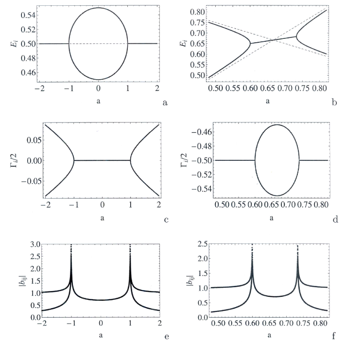
Figure 1: Energies $E_{i}$, widths $\Gamma_{i}/2$ and wavefunctions $|b_{ij}|$ of $N=2$ states coupled to $K=1$ channel as function of $a$ of a PT symmetric system with Hamiltonian (28) (left panel) and of an open quantum system with Hamiltonian (6) (right panel). Parameters left panel: $e=0.5;~{}\gamma_{1}=-\gamma_{2}=0.05~{}a;~{}w=0.05$;  right panel: $e_{1}=1-0.5~{}a;~{}e_{2}=a$;  $\gamma_{1}/2=\gamma_{2}/2=0.5;~{}\omega=0.05\;i$. The dashed lines in (a,b) show $e_{i}(a)$.

The main difference of these optical systems to open quantum systems consists in the asymmetry of gain and loss in the first case while the states of an open quantum system can only decay (Im$(\varepsilon_{1,2})<0$ and Im$({\cal E}_{1,2})<0$ for all states). Thus, the modes involved in the non-Hermitian Hamiltonian in optics appear in complex conjugate pairs while this is not the case in an open quantum system. As a consequence, the Hamiltonian for $PT$ symmetric structures in optical lattices may have real eigenvalues in a large parameter range. The $2\times 2$ non-Hermitian Hamiltonian may be written as equivalence ; jopt

$${\cal H}_{PT}=\left(\begin{array}[]{cc}~{}e-i\frac{\gamma}{2}{}&w\\ w^{*}&~{}e+i\frac{\gamma}{2}{}\end{array}\right),$$ (28)

where $e$ stands for the energy of the two modes, $\pm\gamma$ describes gain and loss, respectively, and the coupling coefficients $w$ stand for the coupling of the two modes via the lattice. When the $PT$ symmetric optical lattices are studied with vanishing gain, the Hamiltonian reads

$${\cal H}_{PT}^{\prime}=\left(\begin{array}[]{cc}~{}~{}e-i\frac{\gamma}{2}{}{}&w\\ w^{*}&e\end{array}\right)\;.$$ (31)

In realistic systems, $w$ in (28) and (31) is mostly real (or almost real) kottos2 .

The eigenvalues of the Hamiltonian (28) differ from (7),

$${\cal E}^{PT}_{\pm} = e\pm\frac{1}{2}\sqrt{4|w|^{2}-\gamma^{2}}\equiv e\pm Z_{PT}\,.$$ (32)

A similar expression is derived in mumbai1 . Since $e$ and $\gamma$ are real, the ${\cal E}^{PT}_{\pm}$ are real when $4|w|^{2}>\gamma^{2}$. Under this condition, the two levels repel each other in energy what is characteristic of discrete interacting states. The level repulsion decreases with increasing $\gamma$ (when the interaction $w$ is fixed). When $4|w|^{2}=\gamma^{2}$ the two states cross. Here, ${\cal E}^{PT}_{\pm}=e$ and $\gamma=\pm\sqrt{4|w|^{2}}$. With further increasing $\gamma$ and $4|w|^{2}<\gamma^{2}$ ($w$ fixed for illustration), width bifurcation (PT symmetry breaking) occurs and ${\cal E}^{PT}_{\pm}=e\pm\frac{i}{2}\sqrt{\gamma^{2}-4|w|^{2}}$.

These relations are in accordance with (10) to (12) for open quantum systems. Two EPs exist according to

$$4|w|^{2}=(\pm\gamma)^{2}\;.$$ (33)

Further

$$\gamma^{2}<4\,|w|^{2} \rightarrow ~{}Z_{PT}~{}\in~{}\Re$$ (34)

$$\gamma^{2}>4\,|w|^{2} \rightarrow ~{}Z_{PT}~{}\in~{}\Im$$ (35)

independent of the parameter dependence $\gamma(a)$ and of the ratio Re$(w)$/Im$(w)$.

In the case of the Hamiltonian (31), the eigenvalues read

$${\cal E}^{{}^{\prime}PT}_{\pm}=e-i~{}\frac{\gamma}{4}\pm\frac{1}{2}\sqrt{4|w|^{2}-\frac{\gamma^{2}}{4}}\equiv e-i~{}\frac{\gamma}{4}\pm Z_{PT}^{\prime}.$$ (36)

We have level repulsion as long as $4|w|^{2}>\frac{\gamma^{2}}{4}$. While level repulsion decreases with increasing $\gamma$, loss increases with increasing $\gamma$. At the crossing point, ${\cal E}^{{}^{\prime}PT}_{\pm}=e-i~{}\frac{\gamma}{4}$. With further increasing $\gamma$ and $4|w|^{2}\ll\frac{\gamma^{2}}{4}$

$${\cal E}^{{}^{\prime}PT}_{\pm}\to e-i~{}\frac{\gamma}{4}\pm i~{}\frac{\gamma}{4}=\Bigg{\{}\begin{array}[]{c}e\\ e-i~{}\frac{\gamma}{2}.\end{array}$$ (39)

The two modes (39) behave differently. While the loss in one of them is large, it is almost zero in the other one. Thus, only one of the modes effectively survives. Equation (39) corresponds to high transparency at large $\gamma$.

Further, two EPs exist according to

$$4|w|^{2}=(\pm\gamma/2)^{2}$$ (40)

and

$$\gamma^{2}/4<4\,|w|^{2} \rightarrow ~{}Z_{PT}^{{}^{\prime}}~{}\in~{}\Re$$ (41)

$$\gamma^{2}/4>4\,|w|^{2} \rightarrow ~{}Z_{PT}^{{}^{\prime}}~{}\in~{}\Im\;.$$ (42)

In analogy to (33) up to (35)), these relations are independent of the parameter dependence of $\gamma$ and of the ratio Re$(w)$/Im$(w)$.

Thus, the difference between the eigenvalues ${\cal E}_{i}$ of ${\cal H}^{(2)}$ of an open quantum system and the eigenvalues of the Hamiltonian of a PT symmetric system consists, above all, in the fact that the ${\cal E}_{i}$ depend on the ratio Re$(\omega)$/Im$(\omega)$ while the ${\cal E}^{PT}_{\pm}$ and ${\cal E}^{{}^{\prime}PT}_{\pm}$ are independent of Re$(w)$/Im$(w)$. There exist however similarities between the two cases.

Interesting is the comparison of the eigenvalues ${\cal E}_{i}$ of ${\cal H}^{(2)}$ obtained for imaginary non-diagonal matrix elements $\omega$, with the eigenvalues of (28) (or (31)) obtained for real $w$. In both cases, there are two EPs, see Fig. 1. In the first case (right panel), the energies $E_{i}$ of both states are equal and the widths $\Gamma_{i}$ bifurcate between the two EPs. This situation is characteristic of an open quantum system at high level density with complex (almost imaginary) $\omega$, see Eqs. (10) to (12). In the second case (left panel) however the difference $|E_{1}-E_{2}|$ of the energies increases (level repulsion) first and decreases then again while the widths $\Gamma_{i}$ of both states vanish in the parameter range between the two EPs in accordance with the analytical results (33) to (35). Between the two EPs, level repulsion causes the two levels to be distant from one another and $w$ is expected to be (almost) real. This result agrees qualitatively with (2) and (3). Similar results are obtained for the eigenvalues of (31). The only difference to those of (28) is that the $\Gamma_{i}$ do not vanish but decrease between the two EPs with increasing $a$ in this case.

According to Figs. 1.a-d, the role of energy and width is formally exchanged when the eigenvalues of the Hamiltonian (6) are compared with those of (28) (or (31)). In any case, the eigenvalues are influenced strongly by the EPs.

Also the eigenfunctions of the Hamiltonian (6) of an open quantum system (with imaginary $\omega$) and those of the Hamiltonians (28) and (31) of a PT symmetric system (with real $w$) show similar features. The eigenfunctions $\Phi_{i}^{PT}$ of ${\cal H}_{PT}$ (and $\Phi_{i}^{{}^{\prime}PT}$ of ${\cal H}_{PT}^{\prime}$) are biorthogonal with all the consequences discussed in Sect. II. In contrast to the eigenvalues, they are dependent on the ratio Re$(\omega)$/Im$(\omega)$.

The eigenfunctions can be represented in a set of basic wavefunctions in full analogy to the representation of the eigenfunctions $\Phi_{i}$ of ${\cal H}^{(2)}$ in (24). They contain valuable information on the mixing of the wavefunctions under the influence of the non-diagonal coupling matrix elements $w$ and $w^{*}$ in (28) and (31), respectively, and its relation to EPs. Due to the level repulsion occurring between the two EPs, the coupling coefficients $w$ can be considered to be (almost) real in realistic cases. The phases of the eigenmodes of the non-Hermitian Hamiltonians (28) and (31) are not rigid, generally, in approaching an EP, and spectroscopic redistribution processes occur in the system under the influence of the environment (lattice). As in the case of open quantum systems, the phase rigidity $r_{k}$ can be defined according to (25). It varies between 1 and 0 and is a quantitative measure for the skewness of the modes when the crossing point is approached.

In Figs. 1.e and f, the eigenfunctions of the Hamiltonian (28) (calculated with real $w$) are compared to those of the Hamiltonian (6) (calculated with imaginary $\omega$). They show the same characteristic features. As can be seen from Fig. 1.e, PT symmetry breaking is accompanied by a mixing of the eigenfunctions in a finite neighborhood of the EPs in PT symmetric systems. This result is in complete analogy to the results shown in Fig. 1.f for open quantum systems where a hint to width bifurcation can be seen in the mixing of the eigenfunctions around these points. Also the phases of the eigenfunctions jump in both cases by $\pi/4$ at the EPs (not shown here). In the parameter region between the two EPs, the eigenfunctions are completely mixed (1:1) in both cases while they are unmixed far beyond the EPs, see Figs. 1.e and f.

IV Discussion of the results

On the basis of $2\times 2$ models, we have compared the influence of an EP onto the dynamics of an open quantum system with its influence onto PT symmetry breaking in a PT symmetric system. In the first case the coupling of the two states via the environment is symmetric ($\omega_{12}=\omega_{21}\equiv\omega$). In the second case however, the formal equivalence of the optical wave equation in PT symmetric optical lattices with a quantum mechanical Schrödinger equation causes the two nondiagonal matrix elements to be complex conjugate ($w_{21}=w_{12}^{*}$). The eigenvalues depend in the first case on the ratio Re${(\omega)}$/Im${(\omega)}$ while they are independent of Re${(w)}$/Im${(w)}$ in the second case. The eigenfunctions are sensitive to Re${(\omega)}$/Im${(\omega)}$ and Re${(w)}$/Im${(w)}$, respectively, in both cases.

The EPs cause nonlinear effects in their neighborhood which determine the evolution of open as well as of PT symmetric systems. Most important for the dynamics of an open quantum system is the regime at high level density where the coupling coefficients are (almost) imaginary. Here, two EPs appear when the decay widths $\gamma_{i}$ of both states are (almost) the same. Approaching the EPs, width bifurcation starts and ends, respectively, while beyond the EPs the widths of both states are equal (or similar) to one another. The energies of the two states show an opposite behavior: it is $E_{i}=E_{2}$ (or $E_{i}\approx E_{2}$) in the parameter range between the two EPs while the states repel each other in energy beyond the EPs. The width bifurcation related to the two EPs becomes relevant for the dynamics of an open quantum system at high level density. Here, short-lived and long-lived states are formed which are related to different time scales of the system (for details see fdp1 ).

Two EPs appear also in a PT symmetric system, and PT symmetry breaking is directly related to them. From a mathematical point of view however, energy and time are exchanged in comparison with the corresponding values in an open quantum system. That means the widths of both states are equal and vanish in the case of the Hamiltonian (28) with gain and loss in the whole parameter range between the two EPs. In this parameter range, the eigenvalues are real and, furthermore, level repulsion prohibits a small energy distance between the two levels. Therefore the non-diagonal coupling matrix elements $w$ are (almost) real, Re$(w)\gg{\rm Im}(w)$.

The eigenfunctions of the different $2\times 2$ models considered in the present paper, show very clearly that the spectroscopic redistribution inside the system is caused by the EPs, indeed. However, it shows up in all cases in a finite neighborhood around them. Here the rigidity of the phases of the two eigenfunctions relative to one another is reduced ($r_{i}<1$) and an alignment of one of the states to the environment is possible. In the parameter range between the two EPs, the wavefunctions are completely mixed (1:1) as can be seen from the numerical results shown in Fig. 1.

Summing up the discussion we state the following. The results obtained by studying PT symmetric optical lattices as well as those received from an investigation of open quantum systems show the characteristic features of non-Hermitian quantum physics. They prove environmentally induced effects that cannot be described convincingly in conventional Hermitian quantum physics. Due to the reduced phase rigidity around an EP, the system is able to align (at least partly) with the environment. This can be seen from PT symmetry breaking occurring in one of the considered systems as well as from the dynamical phase transition taking place at high level density in the other system.

References

- (1) Bender, C.M., and Boettcher, S.: Real Spectra in Non-Hermitian Hamiltonians Having PT Symmetry, Phys. Rev. Lett. 80 (1998) 5243-5246
- (2) Bender, C.M.: Making sense of non-Hermitian Hamiltonians, Rep. Progr. Phys. 70 (2007) 947-1018
- (3) Special Issue Quantum physics with non-Hermitian operators, J. Phys. A 45, Number 44 (November 2012)
-
(4)
Ruschhaupt, A., Delgado, F. and Muga, J.G.:
Physical realization of PT symmetric potential scattering in a planar
slab waveguide,
J. Phys. A 38 (2005) L171-L176;
El-Ganainy, R., Makris, K.G., Christodoulides, D.N. and Musslimani, Z.H.: Theory of coupled optical PT-symmetric structures, Optics Lett. 32 (2007) 2632-2634;
Makris, K.G., El-Ganainy, R., Christodoulides, D.N. and Musslimani, Z.H.: Beam Dynamics in PT Symmetric Optical Lattices, Phys. Rev. Lett. 100 (2008) 103904 (4pp);
Musslimani, Z.H., Makris, K.G., El-Ganainy, R. and Christodoulides, D.N.: Optical Solitons in PT Periodic Potentials, Phys. Rev. Lett. 100 (2008) 030402 (4pp) - (5) Guo, A., Salamo, G.J., Duchesne, D., Morandotti, R., Volatier-Ravat, M., Aimez, V., Siviloglou, G.A., and Christodoulides, D.N.: Observation of PT-symmetry breaking in complex optical potentials, Phys. Rev. Lett. 103 (2009) 093902 (4pp)
- (6) Rüter, C.E., Makris, G., El-Ganainy, R., Christodoulides, D.N., Segev, M., and Kip, D.: Observation of parity-time symmetry in optics, Nature Physics 6 (2010) 192-195
- (7) Kottos, T.: Broken symmetry makes light work, Nature Physics 6 (2010) 166-167
-
(8)
Feshbach, H.:
Unified theory of nuclear reactions,
Ann. Phys. (N.Y.) 5 (1958) 357-390;
Feshbach, H.: A unified theory of nuclear reactions. II, Ann. Phys. (N.Y.) 19 (1962) 287-313 - (9) I. Rotter: A continuum shell model for the open quantum mechanical nuclear system, Rep. Prog. Phys. 54 (1991) 635-682
- (10) Rotter, I.: A non-Hermitian Hamilton operator and the physics of open quantum systems, J. Phys. A 42 (2009) 153001 (51pp)
- (11) Kato, T.: Peturbation Theory for Linear Operators Springer Berlin, 1966
- (12) Rotter, I.: Environmentally induced effects and dynamical phase transitions in quantum systems, J. Opt. 12 (2010) 065701 (9pp)
-
(13)
Landau, L.,
Physics Soviet Union 2, 46 (1932);
Zener, C.: Non-Adiabatic Crossing of Energy Levels, Proc. Royal Soc. London, Series A 137 (1932) 696-702 - (14) Rotter, I.: Dynamical stabilization and time in open quantum systems, Contribution to the Special Issue Quantum Physics with Non-Hermitian Operators: Theory and Experiment, Fortschritte der Physik - Progress of Physics 61 No. 2-3 (2013) 178-193
- (15) Müller, M., Dittes, F.M., Iskra, W. and Rotter, I.: Level repulsion in the complex plane, Phys. Rev. E 52 (1995) 5961-5973
- (16) In studies by other researchers, the factor in (18) does not appear. This difference is discussed in detail and compared with experimental data in the Appendix of fdp1 and in section 2.5 of top
- (17) Rotter, I.: Dynamics of quantum systems, Phys. Rev. E 64 (2001) 036213 (12pp)
- (18) Eleuch, H. and Rotter, I.: Width bifurcation and dynamical phase transitions in open quantum systems, Phys. Rev. E 87 (2013) 052136 (15pp); Eleuch, H. and Rotter, I.: Avoided level crossings in open quantum systems, Contribution to the Special Issue Quantum Physics with Non-Hermitian Operators: Theory and Experiment, Fortschritte der Physik - Progress of Physics 61 No. 2-3 (2013) 194-204. In difference to these papers, the definitions and (with and for decaying states) are used in the present paper.
- (19) Eleuch, H. and Rotter, I., Eur. Phys. J. D 68 (2014) 74 (16pp)
- (20) Kottos, T., private communication