$K$-theoretic boson-fermion correspondence and melting crystals

Abstract

We study non-Hermitian integrable fermion and boson systems from the perspectives of Grothendieck polynomials. The models considered in this article are the five-vertex model as a fermion system and the non-Hermitian phase model as a boson system. Both of the models are characterized by the different solutions satisfying the same Yang-Baxter relation. From our previous works on the identification between the wavefunctions of the five-vertex model and Grothendieck polynomials, we introduce skew Grothendieck polynomials, and derive the addition theorem among them. Using these relations, we derive the wavefunctions of the non-Hermitian phase model as a determinant form which can also be expressed as the Grothendieck polynomials. Namely, we establish a $K$-theoretic boson-fermion correspondence at the level of wavefunctions. As a by-product, the partition function of the statistical mechanical model of a 3D melting crystal is exactly calculated by use of the scalar products of the wavefunctions of the phase model. The resultant expression can be regarded as a $K$-theoretic generalization of the MacMahon function describing the generating function of the plane partitions, which interpolates the generating functions of two-dimensional and three-dimensional Young diagrams.

1 Introduction

The symmetric polynomials is the basic object in representation theory, combinatorics and related geometry. It also appears in mathematical physics, especially in the integrable models. The most fundamental symmetric polynomial is the Schur polynomials, which appears as the solutions of the KP hierarchy [1] and wavefunctions of the phase model [2, 3, 4, 5, 6, 7] for example. It can also be used to construct a determinantal process named the Schur process [8] which have applications to the partition functions of the topological strings [9], for example.

We recently extended the relation between the Schur polynomials and the integrable models, and found that the wavefunctions of the one-parameter family of the integrable five-vertex models can be represented in Grothendieck polynomials [10]. The Grothendieck polynomials was originally introduced in the context of algebraic geometry [11, 12, 13, 14] as structure sheaf of the Schubert variety in the $K$-theory of flag varieties. By the identification of the wavefunctions with the Grothendieck polynomials for Grassmannian varieties, the determinant representations of the scalar products, which is the inner product between the wavefunctions, is nothing but the Cauchy identity for the Grothendieck polynomials. We also revealed the meaning of the orthogonality to show that the Grothendieck polynomials is a discrete orthogonal polynomial over the “Cassini oval” [15], the solution curve of the Bethe equations.

The integrable five-vertex model is related to the non-Hermitian quantum integrable spin chain and the stochastic process called the totally asymmetric simple exclusion process (TASEP) [16]. The TASEP is a many-particle stochastic process with exclusion as an interaction, which can be viewed as a natural generalization of random walk. From the following perspectives, these models can be regarded as fermion systems. First, the space on which the Hamiltonian or the stochastic matrix acts is the tensor product of copies of two-dimensional space spanned by the empty state and particle-occupied state, i.e. the double occupancy is forbidden. Second, the above models are in one-to-one correspondence with fermion systems through the Jordan-Wigner transformation. Finally for the interaction-free case, the physical quantities, such as wavefunctions, and the number of configurations of stochastic particles, etc. are represented as the Schur polynomials which can be described in terms of the formalism of the fermion and its Fock space.

In this paper, we study another type of integrable lattice model derived by a different solution satisfying the same Yang-Baxter relation for the five-vertex model. The model discussed in this paper is a boson model called the non-Hermitian phase model [17], which is a one-parameter generalization of the phase model [18]. At a special point of the parameter, the non-Hermitian phase model describes the totally asymmetric zero range process (TAZRP), i.e., a stochastic process for a system of bosons which, in contrast to the TASEP, the particles are allowed to occupy the same site. The wavefunctions of the phase model was shown to be expressed as the Schur polynomials [2]. In this sense, the phase model can be interpreted as the free fermion systems. We show that the one-parameter family of the phase model corresponds to the generalization from the Schur polynomials to the Grothendieck polynomials. Namely, we show that the wavefunctions of the non-Hermitian phase model is nothing but the Grothendieck polynomials: we establish a $K$-theoretic boson-fermion correspondence at the level of the wavefunctions. We show this by introducing the skew Grothendieck polynomials and by deriving an addition theorem satisfied by the skew Grothendieck polynomials. The skew Grothendieck polynomials can be introduced in the context of the integrable five-vertex model naturally from the relation between the wavefunctions of the $N$-particle state and the $N$-variable Grothendieck polynomials (see [19, 14] for another definition introduced from perspectives of combinatorics). By this boson-fermion correspondence, the determinant representations of the scalar products and the summation of the wavefunctions follow from the Cauchy identity and the summation formula for the Grothendieck polynomials. The Cauchy identity [10] used in this paper is different from the dual Cauchy identity [20] which is the pairing between Grothendieck polynomials and dual Grothendieck polynomials. Our approach is based on the quantum inverse scattering method which starts from the $L$-operator. There is another approach to the wavefunction from the coordinate Bethe ansatz [21], where the equivalence with the Grothendieck polynomials follows as a consequence.

As another application of the above mentioned boson-fermion correspondence, we study the statistical mechanical model of a three-dimensional melting crystal. The model is in one-to-one correspondence with the plane partitions which is regarded as a three-dimensional extension of the Young diagrams. The partition function of the model becomes a generating function of the plane partitions. We show the partition function can be exactly calculated by the scalar product of the non-Hermitian phase model. For the finite volume, the partition function can be given by a determinant form which reproduces MacMahon’s generating function [22] at a special point of the parameter. In the infinite volume limit, the partition function is explicitly given by an infinite product which is regarded as a $K$-theoretic generalization of the MacMahon function [22]. The $K$-theoretic MacMahon function interpolates the ordinary MacMahon function and Euler’s generating function of partitions. Namely, it unifies the generating functions of the two-dimensional and three-dimensional Young diagrams. Note that there are other types of three-dimensional melting crystal models [23, 24, 25, 26] whose constructions are based on connections with integrable models such as the loop models related to the XXZ chain at roots of unity and free fermion models, or connections with symmetric polynomials such as the Schur polynomials and its generalization to the Hall-Littlewood and the Macdonald polynomials. Our model is different from them, and is based on the non-Hermitian integrable spin chain and phase model, whose wavefunctions are the Grothendieck polynomials. The directions of extending the Schur polynomials to the Grothendieck and Macdonald polynomials are different, hence the explicit forms of the corresponding skew polynomials and the weights assigned to each plane partition are totally different between the one in this paper and the ones in previous literature. The Hall-Littlewood polynomials have representations in terms of vertex operators, and many properties including the connection with the melting crystal model can be treated in the same way for the Schur polynomials. However, there is no such vertex operator representation for the Grothendieck polynomials, and we approach to the problem of construction by using the correspondence with the non-Hermitian integrable models.

This paper is organized as follows. In the next section, we review the relation between the wavefunctions of the integrable five-vertex model and the Grothendieck polynomials. In section 3, we introduce the skew Grothendieck polynomials and derive an addition theorem satisfied by them. In section 4, we introduce the non-Hermitian phase model, and show that the wavefunctions can be expressed as Grothendieck polynomials in section 5. In section 6, we discuss the melting crystal and derive the exact expressions of the partition function of the model. Section 7 is devoted to summary and discussion.

2 Grothendieck polynomials and five-vertex models

In this section, we recall a relationship between Grothendieck polynomials and the integrable five-vertex model [10]. Utilizing this relation, in the next section we introduce skew Grothendieck polynomials which play a key role in subsequent analysis.

Grothendieck polynomials were originally introduced as polynomial representatives of structure sheaf of the Schubert variety in the $K$-theory of flag varieties [11]. The $\beta$-Grothendieck polynomials was introduced [12] to unify the original Grothendieck polynomials and the Schubert polynomials, which are structure sheaves for the $K$-theory ($\beta=-1$) and the cohomology ($\beta=0$), respectively. For the case when the flag variety is type $A$ Grassmannian varieties, the Grothendieck polynomials can be represented as the following determinant form [13], which we regard as the definition of the Grothendieck polynomials.

Definition 2.1.

[11, 12, 13] The Grothendieck polynomials is defined as the following determinant

$$G_{\lambda}(z_{1},\dots,z_{N};\beta)=\frac{\mathrm{det}_{N}(z_{j}^{\lambda_{k}+N-k}(1+\beta z_{j})^{k-1})}{\prod_{1\leq j<k\leq N}(z_{j}-z_{k})},$$ (2.1)

where $\{z_{1},\dots,z_{N}\}$ is a set of variables and $\lambda=(\lambda_{1},\dots,\lambda_{N})$ is a sequence of weakly decreasing nonnegative integers $\lambda_{1}\geq\dots\geq\lambda_{N}\geq 0$.

Note that for the case of cohomology $\beta=0$, the $\beta$-Grothendieck polynomials are nothing but the Schur polynomials, which are Schubert polynomials for type $A$ grassmannian varieties.

In fact, the Grothendieck polynomials appear as wave-functions in the five-vertex model. The five-vertex model is a two-dimensional statistical mechanical model whose Boltzmann weights are given by the elements of the $L$-operator [10] $L_{aj}(u)\in\operatorname{End}(W_{a}\otimes V_{j})$:

$$L_{aj}(u)=us_{a}s_{j}+\sigma_{a}^{-}\sigma_{j}^{+}+\sigma_{a}^{+}\sigma_{j}^{-}+(-\beta^{-1}u-u^{-1})n_{a}s_{j}-\beta^{-1}un_{a}n_{j}\quad(u\in\mathbb{C}),$$ (2.2)

where $W_{a}=\mathbb{C}^{2}$ (resp. $V_{j}=\mathbb{C}^{2}$) denotes the $a$th auxiliary space (resp. $j$th quantum space) spanned by the empty state $|0\rangle_{a}=\binom{1}{0}_{a}$ (resp. $|0\rangle_{j}=\binom{1}{0}_{j}$) and particle occupied state $|1\rangle_{a}=\binom{0}{1}_{a}$ (resp. $|1\rangle_{j}=\binom{0}{1}_{j}$). The parameter $\beta$ can be taken arbitrary (the parameter $\alpha$ in [10] corresponds to $\beta$ as $\alpha=-\beta^{-1}$). See also Figure 1 for a pictorial description of the $L$-operator (2.2). The above $L$-operator is given by a solution to the following Yang-Baxter relation ($RLL$-relation):

$$R_{ab}(u,v)L_{aj}(u)L_{bj}(v)=L_{bj}(v)L_{aj}(u)R_{ab}(u,v)$$ (2.3)

holding in $\operatorname{End}(W_{a}\otimes W_{b}\otimes V_{j})$ for arbitrary $u,v\in\mathbb{C}$. Here the matrix $R_{ab}(u,v)\in\operatorname{End}(W_{a}\otimes W_{b})$ is defined by

$$R(u,v)=\begin{pmatrix}f(v,u)&0&0&0\\ 0&0&g(v,u)&0\\ 0&g(v,u)&1&0\\ 0&0&0&f(v,u)\end{pmatrix},\,\,f(v,u)=\frac{u^{2}}{u^{2}-v^{2}},\,g(v,u)=\frac{uv}{u^{2}-v^{2}},$$ (2.4)

which is a solution to the Yang-Baxter equation:

$$R_{ab}(u,v)R_{ac}(u,w)R_{bc}(v,w)=R_{bc}(v,w)R_{ac}(u,w)R_{ab}(u,v).$$ (2.5)

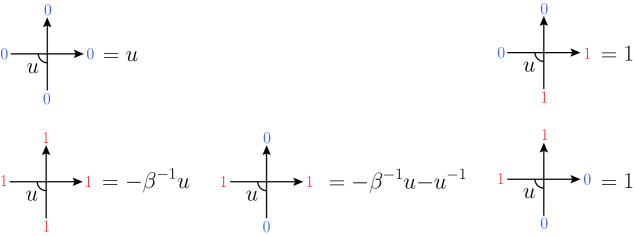
Figure 1: The non-zero elements of the $L$-operator (2.2). The left (resp. up) arrow represents an auxiliary space (resp. a quantum space). The indices 0 or 1 on the left (resp. right) of the vertices denote the input (resp. output) states $|0\rangle$ or $|1\rangle$ in the auxiliary space, while those on the bottom (resp. top) denote the input (resp. output) states in the quantum space. Note that the weights are invariant under a $180^{\circ}$ rotation.

Let us define the monodromy matrix $T(u)$ as a product of $L$-operators:

$$T_{a}(u)=L_{aM}(u)\cdots L_{a1}(u) =\begin{pmatrix}A(u)&B(u)\\ C(u)&D(u)\end{pmatrix}_{a}$$ (2.6)

acting on $W_{a}\otimes(V_{1}\otimes\dots\otimes V_{M})$. Tracing out the auxiliary space, one obtains the transfer matrix $t(u)\in\operatorname{End}(V^{\otimes M})$

$$t(u)=\operatorname{Tr}_{W_{a}}T_{a}(u)$$ (2.7)

which commutes for different spectral parameters: $[t(u),t(v)]=0$. The quantum Hamiltonian corresponding to the five-vertex model is defined by $t(u)$:

$$H:=\sum_{j=1}^{M}\left\{-\beta^{-1}\sigma_{j}^{+}\sigma_{j+1}^{-}+\frac{1}{4}(\sigma_{j}^{z}\sigma_{j+1}^{z}-1)\right\}=\left.\frac{\sqrt{-\beta}}{2}\frac{{\partial}}{{\partial}u}\log\left\{u^{-M}t(u)\right\}\right|_{u=\sqrt{-\beta}}.$$ (2.8)

Note that the above Hamiltonian, in general, is non-Hermitian. For $\beta=-1$, the Hamiltonian corresponds to a stochastic matrix describes a stochastic process called the totally asymmetric simple exclusion process (TASEP).

The arbitrary $N$-particle state $|\psi(\{u\}_{N})\rangle$ (resp. its dual $\langle\psi(\{u\}_{N})|$) (not normalized) with $N$ spectral parameters $\{u\}_{N}=\{u_{1},\dots,u_{N}\}$ is constructed by a multiple action of $B$ (resp. $C$) operator on the vacuum state $|\Omega\rangle:=|0^{M}\rangle:=|0\rangle_{1}\ \otimes\dots\otimes|0\rangle_{M}$ (resp. $\langle\Omega|:=\langle 0^{M}|:={}_{1}\langle 0|\otimes\dots\otimes{}_{M}\langle 0|$):

$$|\psi(\{u\}_{N})\rangle=\prod_{j=1}^{N}B(u_{j})|\Omega\rangle,\quad\langle\psi(\{u\}_{N})|=\langle\Omega|\prod_{j=1}^{N}C(u_{j}).$$ (2.9)

In [10], we computed the overlap between the arbitrary off-shell $N$-particle state $|\psi(\{u\}_{N})\rangle$ and the (normalized) state with an arbitrary particle configuration $|x_{1}\cdots x_{N}\rangle$ $(x_{1}<\dots<x_{N}$), where $x_{j}$ denotes the positions of the particles. The wavefunction $\langle x_{1}\cdots x_{N}|\psi(\{u\}_{N})\rangle$ and its dual $\langle\psi(\{u\}_{N})|x_{1}\cdots x_{N}\rangle$ were found to be given by the Grothendieck polynomials.

Theorem 2.2.

[10] The (off-shell) wavefunction and its dual wave-function of the integrable five-vertex model are, respectively, given by the Grothendieck polynomials as

$$\langle x_{1}\cdots x_{N}|\psi(\{u\}_{N})\rangle =(-\beta^{-1})^{N(N-1)/2}\prod_{j=1}^{N}u_{j}^{M-1}G_{\lambda}(z_{1},\dots,z_{N};\beta),$$ (2.10)

$$\langle\psi(\{u\}_{N})|x_{1}\cdots x_{N}\rangle =(-\beta^{-1})^{N(N-1)/2}\prod_{j=1}^{N}u_{j}^{M-1}G_{\lambda^{\vee}}(z_{1},\dots,z_{N};\beta),$$ (2.11)

where $z_{j}=-\beta^{-1}-u_{j}^{-2}$, and $\lambda=(\lambda_{1},\dots,\lambda_{N})$ ($M-N\geq\lambda_{1}\geq\cdots\geq\lambda_{N}\geq 0$) and $\lambda^{\vee}=(\lambda_{1}^{\vee},\dots,\lambda_{N}^{\vee})$ ($M-N\geq\lambda_{1}^{\vee}\geq\cdots\geq\lambda_{N}^{\vee}\geq 0$) are the Young diagrams related to the particle configuration $x=(x_{1},\dots,x_{N})$ as $\lambda_{j}=x_{N-j+1}-N+j-1$ and $\lambda_{j}^{\vee}=M-N+j-x_{j}$, respectively.

Note that the Young diagram $\lambda^{\vee}$ is the complementary part of the Young diagram $\lambda$ in the $N\times(M-N)$ rectangular Young diagram. Let $x_{j}^{\vee}$ be the particle configuration given by $x_{j}^{\vee}=\lambda^{\vee}_{N-j+1}+j$. The particle configurations $x=(x_{1},\dots,x_{N})$ ($x_{j}=\lambda_{N-j+1}+j$) and $x^{\vee}=(x^{\vee}_{1},\dots,x^{\vee}_{N})$ for given $\lambda$ are connected by the relation:

$$(x^{\vee}_{1},\dots,x^{\vee}_{N})=(M-x_{N}+1,\dots,M-x_{1}+1)\text{ for $x_{j}=\lambda_{N-j+1}+j$ and $x^{\vee}_{j}=\lambda^{\vee}_{N-j+1}+j$}.$$ (2.12)

In Figure 2, we denote an example of $\lambda$ and $\lambda^{\vee}$ together with the corresponding particle configurations $x_{j}=\lambda_{N-j+1}+j$ and $x^{\vee}_{j}=\lambda^{\vee}_{N-j+1}+j$. From this, one can intuitively find that the positions of the particles corresponding to $\lambda^{\vee}$ are related to those corresponding to $\lambda$ after a $180^{\circ}$ rotation.

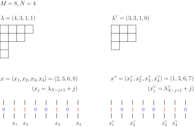
Figure 2: An example of the partitions $\lambda$ and $\lambda^{\vee}$ and the corresponding particle configurations $x$ ($x_{j}=\lambda_{N-j+1}+j$) and $x^{\vee}$ ($x_{j}^{\vee}=\lambda_{N-j+1}^{\vee}+j$) for the conditions $M=8$, $N=4$ and $\lambda=(4,3,1,1)$. One sees that the positions of the particles corresponding to $\lambda^{\vee}$ are related to those corresponding to $\lambda$ after a $180^{\circ}$ rotation.

The graphical description of the wavefunction $\langle x_{1}\cdots x_{N}|\psi(\{u\}_{N})\rangle$ (2.10) is also depicted in Figure 3. Due to the invariance of the Boltzmann weights under a $180^{\circ}$ rotation and $[B(u),B(v)]=0$ ($[C(u),C(v)]=0$), the graphical description of the wavefunction is also invariant under the rotation. One easily finds that the rotated graph corresponds to the dual wavefunction $\langle\psi(\{u_{N}\})|x^{\vee}_{1}\cdots x^{\vee}_{N}\rangle$ where the positions of the particles $x^{\vee}_{j}$ is given by (2.12). After transforming $x^{\vee}\to x$ which corresponds to the transformation $\lambda\to\lambda^{\vee}$, one finds (2.11) is valid if (2.10) holds.

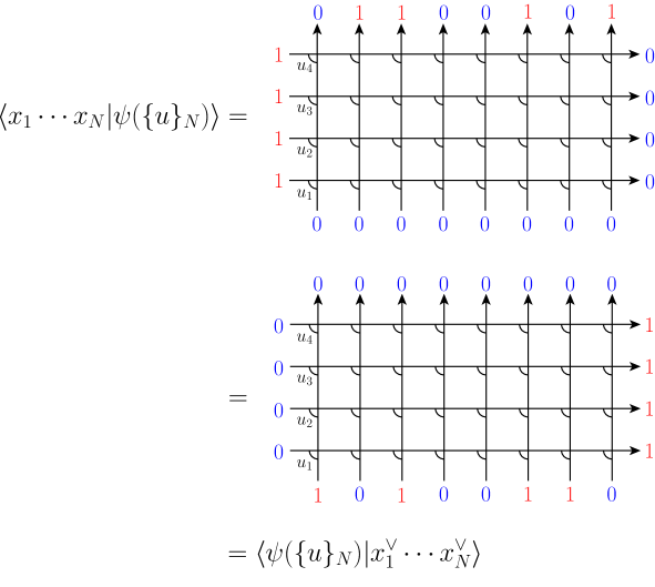
Figure 3: A graphical description of the wavefunction (2.10) for $M=8$, $N=4$ and $\lambda=(4,3,1,1)$ (same conditions in Figure 2). To go from the first equality to the second equality, we use the invariance of the Boltzmann weights under a $180^{\circ}$ rotation and the commutativity of the $B$- and $C$-operators $[B(u),B(v)]=0$ and $[C(u),C(v)]=0$.

One can show the following Cauchy identity holds for the Grothendieck polynomials, which is obtained by comparing the determinant representations for the scalar product $\langle\psi(\{v\}_{N})|\psi(\{u\}_{N})\rangle$ [10] to that obtained by multiplying (2.10) by (2.11) and then by summing over all possible configurations $1\leq x_{1}<\cdots<x_{N}\leq M$.

Theorem 2.3.

[10] The following Cauchy identity for the Grothendieck polynomials holds.

$$\sum_{\lambda\subseteq L^{N}}G_{\lambda}(z_{1},\dots,z_{N};\beta)G_{\lambda^{\vee}}(w_{1},\dots,w_{N};\beta)$$

$$= \prod_{1\leq j<k\leq N}\frac{1}{(z_{j}-z_{k})(w_{k}-w_{j})}\mathrm{det}_{N}\left[\frac{z_{j}^{L+N}(1+\beta w_{k})^{N-1}-w_{k}^{L+N}(1+\beta z_{j})^{N-1}}{z_{j}-w_{k}}\right],$$ (2.13)

where the Young diagram $\lambda^{\vee}=(\lambda_{1}^{\vee},\dots,\lambda_{N}^{\vee})$ is given by the Young diagram $\lambda=(\lambda_{1},\dots,\lambda_{N})$ as $\lambda_{j}^{\vee}=L-\lambda_{N+1-j}$.

Here we have set $L=M-N$, but the above formula holds for any $L\geq 0$. As a limiting case of the Cauchy identity, we have also derived the summation formula for the Grothendieck polynomials.

Theorem 2.4.

[10] The following summation for the Grothendieck polynomials holds.

$$\sum_{\lambda\subseteq L^{N}}(-\beta)^{\sum_{j=1}^{N}\lambda_{j}}G_{\lambda}(z_{1},\dots,z_{N};\beta)=\prod_{1\leq j<k\leq N}\frac{1}{z_{k}-z_{j}}\mathrm{det}_{N}V$$ (2.14)

with an $N\times N$ matrix $V$ whose matrix elements are

$$V_{jk}=\sum_{m=0}^{j-1}(-1)^{m}(-\beta)^{j-N}\binom{L+N}{m}(1+\beta z_{k})^{m-j+N-1}\quad(1\leq j\leq N-1),$$

$$V_{Nk}=-\sum_{m=\mathrm{max}(N-1,1)}^{L+N}(-1)^{m}\binom{L+N}{m}(1+\beta z_{k})^{m-1}.$$ (2.15)

Let us comment on a possible extension of the method to another integrable model also defined by (2.3). In fact, for given $R$-matrix (2.4), the $L$-operator (2.2) is not the unique solution to (2.3). Indeed, the non-Hermitian phase model discussed in section 4 is constructed by another solution to (2.3). As mentioned before, the quantum space on which the $L$-operator (2.2) acts is the tensor product of copies of two-dimensional space spanned by the empty state $|0\rangle$ and particle-occupied states $|1\rangle$, i.e., the double occupancy is forbidden. In this sense, the corresponding quantum system (2.8) is interpreted as a fermion system. (More precisely, there exists a one-to-one correspondence between the spin system (2.8) and a fermion system through the Jordan-Wigner transformation.) On the other hand, the phase model (see (4.4) and (4.5) in section 4) is a boson system: the quantum space is defined as the tensor product of bosonic Fock spaces whose dimension is infinite. At first glance it seems there is little connection between the fermion system (2.8) and the bosonic system (4.4), but by definition the algebraic relations of the both $B$-operators (or $C$-operators) constructing the $N$-particle states are completely the same. Moreover, as shown later, the $N$-particle states for the phase model can be uniquely mapped to those for a fermion model (2.8), and vice versa. These observations intuitively indicate that there is a close correspondence between the fermion (2.8) and the boson (4.4) models. This intuition is true. Indeed, the wavefunctions for the both models can be given by the Grothendieck polynomials. To show this, first we give an addition theorem satisfied by the Grothendieck polynomials, introducing the skew Grothendieck polynomials.

3 Skew Grothendieck polynomials and addition theorem

The relations (2.10) and (2.11) between the wavefunctions and the Grothendieck polynomials lead us to the natural definition of the single variable skew Grothendieck polynomials.

Definition 3.1.

(cf. [19]) The single variable skew Grothendieck polynomial is defined in terms of the $B$-operator of the five-vertex model:

$$G_{\mu/\lambda}(z;\beta):=\langle y_{1}\cdots y_{N+1}|(-\beta)^{N}u^{1-M}B(u)|x_{1}\cdots x_{N}\rangle,$$ (3.1)

where $z=-\beta^{-1}-u^{-2}$, and $\lambda=(\lambda_{1},\dots,\lambda_{N})$ ($M-N\geq\lambda_{1}\geq\cdots\geq\lambda_{N}\geq 0$) and $\mu=(\mu_{1},\dots,\mu_{N+1})$ ($M-N-1\geq\mu_{1}\geq\cdots\geq\mu_{N+1}\geq 0$) are the Young diagrams related to the particle configurations $x=(x_{1},\dots,x_{N})$ ($x_{j}=\lambda_{N-j+1}+j$) and $y=(y_{1},\dots,y_{N+1})$ ($y_{j}=\mu_{N-j+2}+j$), respectively.

We shall see later that this is a natural extension of the skew Schur polynomials.

Proposition 3.2.

The skew Grothendieck polynomial $G_{\mu/\lambda}(z;\beta)$ defined in (3.1) can be given by in terms of the $C$-operator:

$$G_{\mu/\lambda}(z;\beta)=\langle x^{\vee}_{1}\cdots x^{\vee}_{N}|(-\beta)^{N}u^{1-M}C(u)|y_{1}^{\vee}\cdots y_{N+1}^{\vee}\rangle,$$ (3.2)

or equivalently,

$$G_{\mu^{\vee}/\lambda^{\vee}}(z;\beta)=\langle x_{1}\cdots x_{N}|(-\beta)^{N}u^{1-M}C(u)|y_{1}\cdots y_{N+1}\rangle,$$ (3.3)

where the particle positions $x^{\vee}=(x^{\vee}_{1},\dots,x^{\vee}_{N})$ and $y^{\vee}=(y^{\vee}_{1},\dots,y^{\vee}_{N+1})$ are, respectively, defined as $x_{j}^{\vee}=\lambda_{N-j+1}^{\vee}+j$ and $y_{j}^{\vee}=\mu_{N-j+2}^{\vee}+j$.

Proof.

The graphical argument is useful to show (3.2) and (3.3). As discussed in the wavefunctions (see below Theorem 2.2 and Figure 3), the definition (3.1) is invariant under a $180^{\circ}$ rotation. The rotated graph corresponds to $\langle x^{\vee}_{1}\cdots x^{\vee}_{N}|(-\beta)^{N}u^{1-M}C(u)|y_{1}^{\vee}\cdots y_{N+1}^{\vee}\rangle$. Thus we have (3.2). Transforming the variables as $x_{j}^{\vee}\to x_{j}=\lambda_{N-j+1}+j$ ($1\leq j\leq N$) and $y_{j}^{\vee}\to y_{j}=\mu_{N-j+2}+j$ ($1\leq j\leq N+1$) which, respectively, correspond to the transformations $\lambda\to\lambda^{\vee}$ and $\mu\to\mu^{\vee}$, one obtains (3.3). ∎

Let us define the ordering on the Young diagrams for later purpose.

Definition 3.3.

For two Young diagrams $\mu=(\mu_{1},\mu_{2},\dots,\mu_{N+1})$ and $\lambda=(\lambda_{1},\lambda_{2},\dots,\lambda_{N})$, we say that $\mu$ and $\lambda$ interlace, if and only if $\mu_{j}\geq\lambda_{j}\geq\mu_{j+1}$ $(j=1,\dots,N)$, and write this relation as $\mu\succ\lambda$. Correspondingly, we write $y\succ x$ for the particle configurations $y=(y_{1},\dots,y_{N+1})$ ($y_{j}=\mu_{N-j+2}+j$) and $x=(x_{1},\dots,x_{N})$ ($x_{j}=\lambda_{N-j+1}+j$), if and only if $\mu\succ\lambda$ or equivalently $y_{j}\leq x_{j}<y_{j+1}$ $(j=1,\dots,N)$ holds.

In Figure 4 (resp. Figure 5), an example of the interlacing (resp. non-interlacing) partitions and the corresponding particle configurations are depicted. It immediately follows that

$$\mu\succ\lambda\Longleftrightarrow\mu^{\vee}\succ\lambda^{\vee}.$$ (3.4)

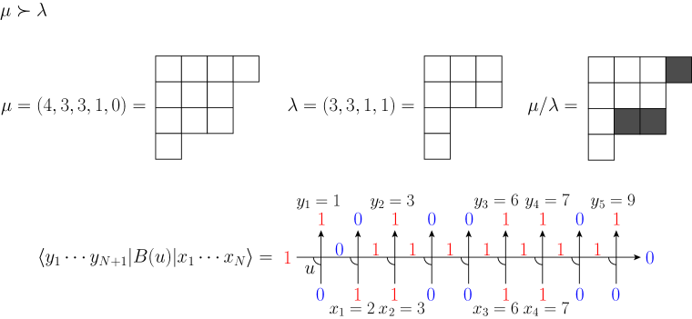
Figure 4: An example of the interlacing partition functions $\mu\succ\lambda$. Here we have set $\mu=(4,3,3,1,0)$ and $\lambda=(3,3,1,1)$. The skew Young diagram $\mu/\lambda$ is depicted as the gray boxes. The input (resp. output) state denotes the particle configuration corresponding to $\lambda$ (resp. $\mu$). For interlacing partitions $\mu\succ\lambda$, the matrix element $\langle y_{1}\cdots y_{N+1}|B(u)|x_{1}\cdots x_{N}\rangle$ is non-zero for the generic value of $u$.

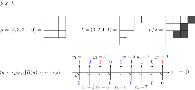
Figure 5: An example of the non-interlacing partition functions $\mu\nsucc\lambda$. Here we have set $\mu=(4,3,3,1,0)$ and $\lambda=(3,2,1,1)$. The input (resp. output) state denotes the particle configuration corresponding to $\lambda$ (resp. $\mu$). For non-interlacing partitions $\mu\nsucc\lambda$, one sees $\langle y_{1}\cdots y_{N+1}|B(u)|x_{1}\cdots x_{N}\rangle=0$.

The single variable skew Grothendieck polynomials (3.1) is given by the following explicit expression.

Proposition 3.4.

The single variable skew Grothendieck polynomials $G_{\mu/\lambda}(z;\beta)$ can be explicitly expressed as

$$G_{\mu/\lambda}(z;\beta)=\begin{cases}z^{\sum_{j=1}^{N+1}\mu_{j}-\sum_{j=1}^{N}\lambda_{j}}\prod_{j=1}^{N}(1+\beta z-\beta z\delta_{\mu_{j+1}\,\lambda_{j}})&\mu\succ\lambda\\ 0&\text{otherwise}\end{cases}.$$ (3.5)

The case $\beta=0$ reduces to the single variable skew Schur polynomials: $G_{\mu/\lambda}(z;0)=s_{\mu/\lambda}(z)=z^{\sum_{j=1}^{N+1}\mu_{j}-\sum_{j=1}^{N}\lambda_{j}}$.

Proof.

We show (3.5) by explicit evaluation of the definition (3.1). From the graphical description (see Figure 5, for instance), we find $\langle y_{1}\cdots y_{N+1}|B(u)|x_{1}\cdots x_{N}\rangle=0$ for $\mu\nsucc\lambda$. Thus $G_{\mu/\lambda}(z;\beta)=0$ holds for $\mu\nsucc\lambda$. The first equality in (3.5) can be shown by the following decomposition:

$$B(u)|x_{1}\cdots x_{N}\rangle={}_{a}\langle 0|\prod_{j=1}^{N+1}\prod_{l=x_{j-1}+1}^{x_{j}}L_{al}(u)|1\rangle_{a}\otimes\left\{\otimes_{k=x_{j-1}+1}^{x_{j}-1}|0\rangle_{k}\right\}\otimes|1\rangle_{x_{j}},$$ (3.6)

where $x_{0}=0$ and $x_{N+1}=M$. Using the following relations,

$$\prod_{l=x_{j-1}+1}^{x_{j}}L_{al}(u)|1\rangle_{a}\otimes\left\{\otimes_{k=x_{j-1}+1}^{x_{j}-1}|0\rangle_{k}\right\}\otimes|1\rangle_{x_{j}}$$

$$\qquad=\sum_{x_{j-1}+1\leq y_{j}\leq x_{j}}(-\beta^{-1}u-u^{-1})^{y_{j}-x_{j-1}-1}\left\{u^{x_{j}-y_{j}-1}(1-\delta_{x_{j}\,y_{j}})-\beta^{-1}u\delta_{x_{j}\,y_{j}}\right\}$$

$$\qquad\quad\times|1\rangle_{a}\otimes\left\{\otimes_{k=x_{j-1}+1}^{y_{j}-1}|0\rangle_{k}\right\}\otimes|1\rangle_{y_{j}}\otimes\left\{\otimes_{k=y_{j}+1}^{x_{j}}|0\rangle_{k}\right\}\qquad(1\leq j\leq N),$$ (3.7)

$${}_{a}\langle 0|\prod_{l=x_{N}+1}^{M}L_{al}(u)|1\rangle_{a}\otimes\left\{\otimes_{k=x_{N}+1}^{M}|0\rangle_{k}\right\}$$

$$\qquad=\sum_{x_{N}+1\leq y_{N+1}\leq M}(-\beta^{-1}u-u^{-1})^{y_{N+1}-x_{N}-1}u^{M-y_{N+1}}$$

$$\qquad\quad\times\left\{\otimes_{k=x_{N}+1}^{y_{N+1}-1}|0\rangle_{k}\right\}\otimes|1\rangle_{y_{N+1}}\otimes\left\{\otimes_{k=y_{N+1}+1}^{M}|0\rangle_{k}\right\},$$ (3.8)

which are directly obtained by the graphical representation shown in Figure 6, we find that (3.6) yields

$$B(u)|x_{1}\cdots x_{N}\rangle= \sum_{y\succ x}(-\beta^{-1}u-u^{-1})^{-1-N+\sum_{j=1}^{N+1}y_{j}-\sum_{j=1}^{N}x_{j}}u^{M-y_{N+1}}$$

$$\times\prod_{j=1}^{N}\{u^{x_{j}-y_{j}-1}(1-\delta_{x_{j}\,y_{j}})-\beta^{-1}u\delta_{x_{j}\,y_{j}}\}|y_{1}\cdots y_{N+1}\rangle.$$ (3.9)

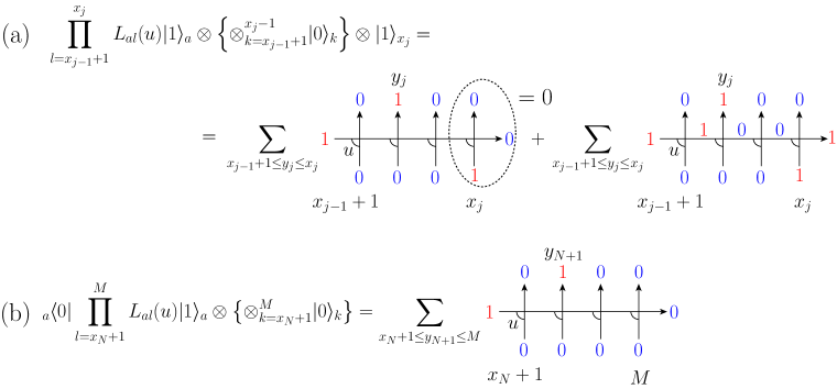
Figure 6: (a): The graphical description of (3.7). The first term of the right hand vanishes because the Boltzmann weight surrounded by the broken line is equal to zero. The insertion of the weights shown in Figure 1 into the second term yields (3.7). (b): The graphical description of (3.8).

Translating (3.9) into the language of Young diagrams by $x_{j}=\lambda_{N-j+1}+j$ and $y_{j}=\lambda_{N-j+2}+j$, and using $y\succ x\Longleftrightarrow\mu\succ\lambda$, we have the first equality in (3.5). ∎

Combining the relation between the wavefunction and the Grothendieck polynomial (2.10) and the definition of the skew Grothendieck polynomials (3.1), we have the following addition theorem.

Theorem 3.5.

The following relation between the Grothendieck and skew Grothendieck polynomials holds

$$G_{\mu}(z_{1},\dots,z_{N},z_{N+1};\beta)=\sum_{\mu\succ\lambda}G_{\mu/\lambda}(z_{N+1};\beta)G_{\lambda}(z_{1},\dots,z_{N};\beta),$$ (3.10)

which recovers the one for the Schur and skew Schur polynomials at $\beta=0$.

Proof.

This follows from evaluating the $(N+1)$-particle state by using (2.10) and (3.1) as

$$(-\beta)^{(N+1)N/2} \prod_{j=1}^{N+1}u_{j}^{1-M}B(u_{j})|\Omega\rangle=(-\beta)^{N}u_{N+1}^{1-M}B(u_{N+1})(-\beta)^{N(N-1)/2}\prod_{j=1}^{N}u_{j}^{1-M}B(u_{j})|\Omega\rangle$$

$$= (-\beta)^{N}u_{N+1}^{1-M}B(u_{N+1})\sum_{\lambda}G_{\lambda}(z_{1},\dots,z_{N};\beta)|x_{1}(\lambda)\cdots x_{N}(\lambda)\rangle$$

$$= \sum_{\mu\succ\lambda}G_{\mu/\lambda}(z_{N+1};\beta)G_{\lambda}(z_{1},\dots,z_{N};\beta)|y_{1}(\mu)\cdots y_{N+1}(\mu)\rangle,$$ (3.11)

and comparing with

$$(-\beta)^{(N+1)N/2}\prod_{j=1}^{N+1}u_{j}^{1-M}B(u_{j})|\Omega\rangle=\sum_{\mu}G_{\mu}(z_{1},\dots,z_{N+1};\beta)|y_{1}(\mu)\cdots y_{N+1}(\mu)\rangle.$$ (3.12)

Note that $\lambda$ in the summation (3.11) can be restricted from $\lambda\subseteq(M-N)^{N}$ to $\lambda\subseteq(M-N-1)^{N}$ since $\mu\subseteq(M-N-1)^{N+1}$ and $G_{\mu/\lambda}(z;\beta)=0$ unless $\mu\succ\lambda$. ∎

The relation (3.10) is the consequence of the action of a $B$-operator on the wavefunction of the $N$-particle state, from which also justifies the definition (3.1) of the skew Grothendieck polynomials. In the next section, we use this addition theorem to show that the wavefunction of the non-Hermitian phase model can also be expressed as Grothendieck polynomials.

The repeated application of the addition theorem (3.10) leads to the following corollary.

Corollary 3.6.

The Grothendieck polynomials can be expressed in terms of the single variable skew Grothendieck polynomials as

$$G_{\lambda}(z_{1},\dots,z_{N};\beta) =\sum_{\lambda=\lambda^{(0)}\succ\lambda^{(1)}\succ\cdots\succ\lambda^{(N)}=\emptyset}\prod_{j=1}^{N}G_{\lambda^{(j-1)}/\lambda^{(j)}}(z_{j};\beta).$$ (3.13)

Before closing this section, we define the multivariable skew Grothendieck polynomials for completeness of the paper. The multivariable skew Grothendieck is naturally defined by multiplying the single variable skew Grothendieck polynomials.

Definition 3.7.

The multivariable skew Grothendieck polynomials is defined as

$$G_{\lambda/\nu}(z_{1},\dots,z_{n};\beta) :=\sum_{\lambda^{(1)}\succ\cdots\succ\lambda^{(n-1)}}\prod_{j=1}^{n}G_{\lambda^{(j-1)}/\lambda^{(j)}}(z_{j};\beta)$$ (3.14)

where $\lambda=\lambda^{(0)}$ and $\nu=\lambda^{(n)}$.

The combination of Corollary 3.6 and Theorem 3.5 leads to the following addition theorem.

Theorem 3.8.

The following relation between the Grothendieck polynomials and the (multivariable) skew Grothendieck polynomials holds:

$$G_{\lambda}(z_{1},\dots,z_{n},w_{1},\dots,w_{m};\beta)=\sum_{\nu}G_{\lambda/\nu}(z_{1},\dots,z_{n};\beta)G_{\nu}(w_{1},\dots,w_{m};\beta),$$ (3.15)

which recovers the one for the Schur and skew Schur polynomials at $\beta=0$.

4 Non-Hermitian phase model

In this section, we introduce the non-Hermitian phase model [17], which can be solved by the algebraic Bethe ansatz. The phase model is a boson system characterized by the generators $\phi$, $\phi^{\dagger}$, $N$ and $\pi$ acting on a bosonic Fock space $\mathcal{F}$ spanned by orthonormal basis $|n\rangle\ (n=0,1,\dots,\infty)$. Here the number $n$ indicates the occupation number of bosons. The generators $\phi$, $\phi^{\dagger}$, $N$ and $\pi$ are, respectively, the annihilation, creation, number and vacuum projection operators, whose actions on $\mathcal{F}$ are, respectively, defined as

$$\phi|0\rangle=0,\quad\phi|n\rangle=|n-1\rangle,\quad\phi^{\dagger}|n\rangle=|n+1\rangle,\quad N|n\rangle=n|n\rangle,\quad\pi|n\rangle=\delta_{n\,0}|n\rangle.$$ (4.1)

Thus the operator forms are explicitly given by

$$\phi=\sum_{n=0}^{\infty}|n\rangle\langle n+1|,\quad\phi^{\dagger}=\sum_{n=0}^{\infty}|n+1\rangle\langle n|,\quad N=\sum_{n=0}^{\infty}n|n\rangle\langle n|,\quad\pi=|0\rangle\langle 0|.$$ (4.2)

These operators generate an algebra referred to as the phase algebra:

$$[\phi,\phi^{\dagger}]=\pi,\quad[N,\phi]=-\phi,\quad[N,\phi^{\dagger}]=\phi^{\dagger}.$$ (4.3)

The non-Hermitian phase model [17, 31] under the periodic boundary condition is defined by the following Hamiltonian:

$$\mathcal{H}=\sum_{j=0}^{M-1}(\phi_{j+1}^{\dagger}\phi_{j}-\beta\pi_{j}).$$ (4.4)

The Hamiltonian acts on the tensor product of Fock spaces $\otimes_{j=0}^{M-1}\mathcal{F}_{j}$, whose basis is given by $|\{n\}_{M}\rangle:=\otimes_{j=0}^{M-1}|n_{j}\rangle_{j}$, $n_{j}=0,1,\dots,\infty$. We denote a dual state of $|\{n\}_{M}\rangle$ as $\langle\{n\}_{M}|:=\otimes_{j=0}^{M-1}{}_{j}\langle n_{j}|$. The operators $\phi_{j}$, $\phi_{j}^{\dagger}$, $N_{j}$ and $\pi_{j}$ act on the Fock space $\mathcal{F}_{j}$ as $\phi$, $\phi^{\dagger}$, $N$ and $\pi$, and the other Fock spaces $\mathcal{F}_{k},k\neq j$ as an identity. The term including $\beta$ in (4.4) denotes an on-site interaction: $\beta>0$, $\beta=0$ and $\beta<0$ correspond to repulsive, free and attractive interactions, respectively.

The Hamiltonian is quantum integrable, and a special point $\beta=-1$ describes a stochastic process without exclusion called the totally asymmetric zero range process (TAZRP), i.e., a stochastic process for a system of bosons so that each site can be occupied by arbitrary number of particles, which is in contrast to the TASEP where each site can be occupied by at most one particle.

We can make an analysis on the non-Hermitian phase model by the quantum inverse scattering method. The basic object is the following $L$ operator

$$\mathcal{L}_{aj}(v)=\begin{pmatrix}v^{-1}-\beta v\pi_{j}&\phi_{j}^{\dagger}\\ \phi_{j}&v\end{pmatrix},$$ (4.5)

acting on the tensor product $W_{a}\otimes\mathcal{F}_{j}$ of the complex two-dimensional space $W_{a}$ and the Fock space at the $j$th site $\mathcal{F}_{j}$. See also Figure 7 for a pictorial representation of the $L$-operator (4.5), which allows for an intuitive understanding of the subsequent calculations. The $L$-operator satisfies the intertwining relation ($RLL$-relation)

$$R_{ab}(u,v)\mathcal{L}_{aj}(u)\mathcal{L}_{bj}(v)=\mathcal{L}_{bj}(v)\mathcal{L}_{aj}(u)R_{ab}(u,v),$$ (4.6)

which acts on $W_{a}\otimes W_{b}\otimes\mathcal{F}_{j}$. The $R$ matrix $R(u,v)$ is the same as the one for the integrable five-vertex model (2.4). The auxiliary space $W_{a}$ is the complex two-dimensional space, which is the same as that for the integrable five-vertex model, while the quantum space $\mathcal{F}_{j}$ is the infinite-dimensional bosonic Fock space.

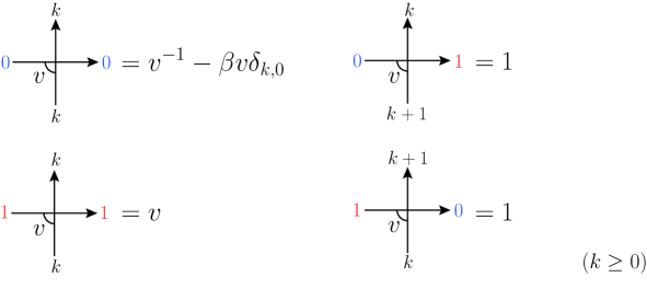
Figure 7: The non-zero elements of the $L$-operator (4.5) for the non-Hermitian phase model. The variables on the left-arrows take $0$ and $1$, since the auxiliary space for the phase model is two-dimensional space which is the same as the one for the five-vertex model. On the other hand, the variables on the up-arrows take infinite values $0,1,\dots,\infty$ which reflects the fact that the quantum space of the phase model is infinite dimensions. Note that the weights are invariant under a $180^{\circ}$ rotation.

From the $L$-operator, we construct the monodromy matrix

$$\mathcal{T}_{a}(v)=\mathcal{L}_{aM-1}(v)\cdots\mathcal{L}_{a0}(v)=\begin{pmatrix}\mathcal{A}(v)&\mathcal{B}(v)\\ \mathcal{C}(v)&\mathcal{D}(v)\end{pmatrix}_{a},$$ (4.7)

which acts on $W_{a}\otimes(\mathcal{F}_{0}\otimes\dots\otimes\mathcal{F}_{M-1})$. Tracing out the auxiliary space, one defines the transfer matrix $\tau(u)\in\mathrm{End}(\mathcal{F}^{\otimes M})$:

$$\tau(v)=\operatorname{Tr}_{W_{a}}\mathcal{T}_{a}(v).$$ (4.8)

The repeated applications of the $RLL$-relation leads to the intertwining relation

$$R_{ab}(u,v)\mathcal{T}_{a}(u)\mathcal{T}_{b}(v)=\mathcal{T}_{b}(v)\mathcal{T}_{a}(u)R_{ab}(u,v).$$ (4.9)

Some elements of the relation (4.9) are

$$\mathcal{C}(u)\mathcal{B}(v)=g(u,v)\left[\mathcal{A}(u)\mathcal{D}(v)-\mathcal{A}(v)\mathcal{D}(u)\right],$$

$$\mathcal{A}(u)\mathcal{B}(v)=f(u,v)\mathcal{B}(v)\mathcal{A}(u)+g(v,u)\mathcal{B}(u)\mathcal{A}(v),$$

$$\mathcal{D}(u)\mathcal{B}(v)=f(v,u)\mathcal{B}(v)\mathcal{D}(u)+g(u,v)\mathcal{B}(u)\mathcal{D}(v),$$

$$\left[\mathcal{B}(u),\mathcal{B}(v)\right]=\left[\mathcal{C}(u),\mathcal{C}(v)\right]=0.$$ (4.10)

The above relations are completely the same as those satisfied by $A(u)$, $B(u)$, $C(u)$ and $D(u)$ for the integrable five-vertex model, since the $RLL$-relation (4.6) is the same as (2.3). Thanks to the $RTT$-relation (4.9), the transfer matrix $\tau(u)$ mutually commutes, i.e.,

$$[\tau(u),\tau(v)]=0.$$ (4.11)

The Hamiltonian can be obtained by the derivative of the transfer matrix with respect to the spectral parameter:

$$\mathcal{H}=\left.\frac{\partial}{\partial v^{2}}(v^{M}\tau(v))\right|_{v=0}.$$ (4.12)

The arbitrary $N$-particle state $|\Psi(\{v\}_{N})\rangle$ (resp. its dual $\langle\Psi(\{v\}_{N})|$) (not normalized) with $N$ spectral parameters $\{v\}_{N}=\{v_{1},\dots,v_{N}\}$ is constructed by a multiple action of $\mathcal{B}$ (resp. $\mathcal{C}$) operator on the vacuum state $|\Omega\rangle:=|0^{M}\rangle:=|0\rangle_{0}\ \otimes\dots\otimes|0\rangle_{M-1}$ (resp. $\langle\Omega|:=\langle 0^{M}|:={}_{0}\langle 0|\otimes\dots\otimes{}_{M-1}\langle 0|$):

$$|\Psi(\{v\}_{N})\rangle=\prod_{j=1}^{N}\mathcal{B}(v_{j})|\Omega\rangle,\quad\langle\Psi(\{v\}_{N})|=\langle\Omega|\prod_{j=1}^{N}\mathcal{C}(v_{j}).$$ (4.13)

The $N$-particle state $|\Psi(\{v\}_{N})\rangle$ and its dual $\langle\Psi(\{v\}_{N})|$ become an eigenvector of the transfer matrix with the eigenvalue

$$\tau(u)=(v^{-1}-\beta v)^{M}\prod_{k=1}^{N}\frac{v_{k}^{2}}{v_{k}^{2}-v^{2}}+v^{M}\prod_{k=1}^{N}\frac{v^{2}}{v^{2}-v_{k}^{2}},$$ (4.14)

if the spectral parameters $\{v\}_{N}$ satisfy the Bethe ansatz equation

$$(v_{j}^{-2}-\beta)^{M}=(-1)^{N-1}\prod_{k=1}^{N}\frac{v_{j}^{2}}{v_{k}^{2}}.$$ (4.15)

The eigenvalue of the Hamiltonian is given by

$$E=-\beta M+\sum_{j=1}^{N}v_{j}^{-2}.$$ (4.16)

5 Wavefunctions and scalar products

Here and in what follows, we consider the arbitrary off-shell state, i.e., the parameters $\{v\}_{N}$ in the $N$-particle state (4.13) are arbitrary. The orthonormal basis of the $N$-particle state $|\Psi(\{v\}_{N})\rangle$ and its dual $\langle\Psi(\{v\}_{N})|$ is given by $|\{n\}_{M,N}\rangle:=|n_{0}\rangle_{0}\ \otimes\dots\otimes|n_{M-1}\rangle_{M-1}$ and $\langle\{n\}_{M,N}|:=_{0}\langle n_{0}|\otimes\dots\otimes_{M-1}\langle n_{M-1}|$, where $n_{0}+n_{1}+\cdots+n_{M-1}=N$. The wavefunctions can be expanded in this basis as

$$|\Psi(\{v\}_{N})\rangle=\sum_{\begin{subarray}{c}0\leq n_{0},\dots,n_{M-1}\leq N\\ n_{0}+\cdots+n_{M-1}=N\end{subarray}}\langle\{n\}_{M,N}|\psi(\{v\}_{N})\rangle|\{n\}_{M,N}\rangle,$$ (5.1)

$$\langle\Psi(\{v\}_{N})|=\sum_{\begin{subarray}{c}0\leq n_{0},\dots,n_{M-1}\leq N\\ n_{0}+\cdots+n_{M-1}=N\end{subarray}}\langle\{n\}_{M,N}|\langle\psi(\{v\}_{N})|\{n\}_{M,N}\rangle.$$ (5.2)

There is a one-to-one correspondence between the set $\{n\}_{M,N}=\{n_{0},n_{1},\dots,n_{M-1}\}$ ($n_{0}+n_{1}+\cdots+n_{M-1}=N$) and the Young diagram $\lambda=(\lambda_{1},\lambda_{2},\dots,\lambda_{N})$ ($M-1\geq\lambda_{1}\geq\lambda_{2}\geq\cdots\geq\lambda_{N}\geq 0$). Namely, each Young diagram $\lambda$ under the constraint $\ell(\lambda)\leq N$, $\lambda_{1}\leq M-1$ can be labeled by a set of integers $\{n\}_{M,N}$ as $\lambda=((M-1)^{n_{M-1}},\dots,1^{n_{1}},0^{n_{0}})$. In Figure 8, we denote the particle positions $\{n\}_{M,N}$ and $\{n^{\vee}\}_{M,N}$, which correspond to the Young diagram $\lambda$ and $\lambda^{\vee}$, respectively. From this, one can intuitively find that the positions of the particles corresponding to $\lambda^{\vee}$ are related to those corresponding to $\lambda$ after a $180^{\circ}$ rotation.

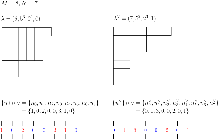
Figure 8: An example of the partitions $\lambda$ and $\lambda^{\vee}$ and corresponding particle configurations $\{n\}_{M,N}=\{n_{0},\dots n_{M-1}\}$ and$\{n^{\vee}\}_{M,N}=\{n^{\vee}_{0},\dots n^{\vee}_{M-1}\}$ for the conditions $M=8$, $N=7$ and $\lambda=(6,5^{3},2^{2},0)$. One sees that the positions of the particles corresponding to $\lambda^{\vee}$ are related to those corresponding to $\lambda$ after a $180^{\circ}$ rotation.

The following definition [6] on the ordering on the basis of particle configurations is useful for later purpose.

Definition 5.1.

[6] For two configurations $\{m\}_{M,N+1}=\{m_{0},m_{1},\dots,m_{M-1}\}$ $(m_{0}+m_{1}+\cdots+m_{M-1}=N+1)$ and $\{n\}_{M,N}=\{n_{0},n_{1},\dots,n_{M-1}\}$ $(n_{0}+n_{1}+\cdots+n_{M-1}=N)$, let $\sum_{j}^{m}=\sum_{k=j}^{M-1}m_{k}$ and $\sum_{j}^{n}=\sum_{k=j}^{M-1}n_{k}$. We say that the particle configurations $\{m\}_{M,N+1}$ and $\{n\}_{M,N}$ are admissible, if and only if $0\leq(\sum_{j}^{m}-\sum_{j}^{n})\leq 1$ ($1\leq j\leq M-1$), and write this relation as $\{m\}_{M,N+1}\triangleright\{n\}_{M,N}$.

Proposition 5.2.

Let $\{m\}_{M,N+1}$ and $\{n\}_{M,N}$ be the particle configurations described by the Young diagram $\mu=(\mu_{1},\dots,\mu_{N+1})$ and $\lambda=(\lambda_{1},\dots,\lambda_{N})$. Then

$$\mu\succ\lambda\Longleftrightarrow\{m\}_{M,N+1}\triangleright\{n\}_{M,N}.$$ (5.3)

In Figure 9 (resp. Figure 10), an example of the interlacing (resp. non-interlacing) partitions and the corresponding admissible (resp. non-admissible) particle configurations are depicted.

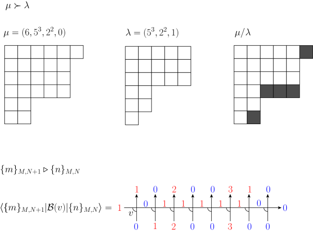
Figure 9: An example of the interlacing partition functions $\mu\succ\lambda$. Here we have set $\mu=(6,5^{3},2^{2},0)$ and $\lambda=(5^{3},2^{2},1)$. The skew Young diagram $\mu/\lambda$ is depicted as the gray boxes. The input (resp. output) state denotes the particle configuration corresponding to $\lambda$ (resp. $\mu$). The particle configurations are admissible for the interlacing partitions. For admissible configurations $\{m\}_{M,N+1}\triangleright\{n\}_{M,N}$, the matrix element $\langle\{m\}_{M,N+1}|\mathcal{B}(v)|\{n\}_{M,N}\rangle$ is non-zero for the generic value of $v$.

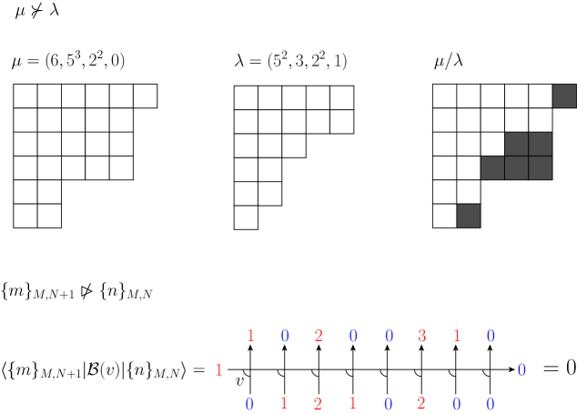
Figure 10: An example of the non interlacing partition functions $\mu\nsucc\lambda$. Here we have set $\mu=(6,5^{3},2^{2},0)$ and $\lambda=(5^{2},3,2^{2},1)$. For non-interlacing partitions, the particle configurations are not admissible. For non-admissible configurations $\{m\}_{M,N+1}\ntriangleright\{n\}_{M,N}$, one sees $\langle\{m\}_{M,N+1}|\mathcal{B}(v)|\{n\}_{M,N}\rangle=0$.

We show the wavefunctions $\langle\{n\}_{M}|\Psi(\{v\}_{N})\rangle$ and its dual $\langle\Psi(\{v\}_{N})|\{n\}_{M}\rangle$ can be represented in the following determinant forms which are parametrized by Young diagrams.

Theorem 5.3.

The wavefunctions can be expressed by the Grothendieck polynomials as

$$\langle\{n\}_{M,N}|\Psi(\{v\}_{N})\rangle=\prod_{j=1}^{N}(v_{j}^{-1}-\beta v_{j})^{M-1}G_{\lambda}(z_{1},\dots,z_{N};\beta),$$ (5.4)

$$\langle\Psi(\{v\}_{N})|\{n\}_{M,N}\rangle=\prod_{j=1}^{N}(v_{j}^{-1}-\beta v_{j})^{M-1}G_{\lambda^{\vee}}(z_{1},\dots,z_{N};\beta),$$ (5.5)

where $z_{j}^{-1}=v_{j}^{-2}-\beta$ and $\lambda^{\vee}=(\lambda_{1}^{\vee},\lambda_{2}^{\vee},\dots,\lambda_{N}^{\vee})$ ($M-1\geq\lambda_{1}^{\vee}\geq\cdots\geq\lambda_{N}^{\vee}\geq 0$) is given by the Young diagram $\lambda$ as $\lambda_{j}^{\vee}=M-1-\lambda_{N+1-j}$.

Proof.

The second relation (5.5) holds if the first equation (5.4) is valid. This follows from an argument similar to that in the wavefunctions for the five-vertex model. Namely, since the Boltzmann weights for the phase model are invariant under a $180^{\circ}$ (see Figure 7) and the commutativity of the $B$- and $C$-operators (4.10), the graphical description of the wave function $\langle\{n\}_{M,N}|\Psi(\{v\}_{N})\rangle$ is also invariant under the rotation (cf. Figure 3 for the five-vertex model). The rotated graph is nothing but the dual wavefunction $\langle\Psi(\{v\}_{N})|\{n^{\vee}\}_{M,N}\rangle$. Transforming $\{n^{\vee}\}\to\{n\}$ which corresponds to the transformation $\lambda\to\lambda^{\vee}$, one finds (5.5) is valid if (5.4) holds. Thus, it is sufficient to show (5.4).

The relation between the wavefunctions of the integrable five-vertex model of $N$ and $N+1$ particles can be reduced to the relation between the Grothendieck and skew Grothendieck polynomials (3.10). This relation is also the key for the non-Hermitian phase model. Namely, we show the following lemma for the correspondence between the matrix elements of the single $\mathcal{B}$- and $\mathcal{C}$- operators and the skew Grothendieck polynomials of a single variable from which one concludes that the wavefunctions is proportional to the Grothendieck polynomials.

Lemma 5.4.

The matrix elements of the single $\mathcal{B}$- and $\mathcal{C}$-operators can be expressed as the skew Grothendieck polynomials of a single variable as

$$\langle\{m\}_{M,N+1}|(v^{-1}-\beta v)^{1-M}\mathcal{B}(v)|\{n\}_{M,N}\rangle =G_{\mu/\lambda}(z;\beta),$$ (5.6)

$$\langle\{n\}_{M,N}|(v^{-1}-\beta v)^{1-M}\mathcal{C}(v)|\{m\}_{M,N+1}\rangle =G_{\mu^{\vee}/\lambda^{\vee}}(z;\beta),$$ (5.7)

where the Young diagram $\mu=(\mu_{1},\mu_{2},\dots,\mu_{N+1})$ $(M-1\geq\mu_{1}\geq\cdots\geq\mu_{N+1}\geq 0)$ is parametrized by the configuration $\{m\}_{M,N+1}=\{m_{0},m_{1},\dots,m_{M-1}\}$ ($m_{0}+\cdots+m_{M-1}=N+1$) as $\mu=((M-1)^{m_{M-1}},\dots,1^{m_{1}},0^{m_{0}})$. The Young diagram $\mu^{\vee}=(\mu_{1}^{\vee},\mu_{2}^{\vee},\dots,\mu_{N+1}^{\vee})$ $(M-1\geq\mu_{1}^{\vee}\geq\cdots\geq\mu_{N+1}^{\vee}\geq 0)$ is given by $\mu_{j}^{\vee}=M-1-\mu_{N+2-j}$.

Here we first end the proof of Theorem 5.3 by using Lemma 5.4. The left hand side of (5.4) is decomposed as

$$\langle\{n\}_{M,N}|\Psi(\{v\}_{N})\rangle$$

$$\quad=\sum_{\{m^{(0)}\},\dots,\{m^{(N-1)}\}}\langle\{n\}_{M,N}|\prod_{j=1}^{N}\left\{\mathcal{B}(v_{j})|\{m^{(N-j)}\}_{M,N-j}\rangle\langle\{m^{(N-j)}\}_{M,N-j}|\right\}|\Omega\rangle.$$ (5.8)

Then applying Lemma 5.4 to the above decomposition and using Corollary 3.6, one obtains (5.4). ∎

Proof of Lemma 5.4. Utilizing the graphical description and an argument similar to Proposition 3.2, one immediately sees that (5.7) automatically holds if (5.6) holds. Let us show (5.6). From the matrix elements of the $L$-operator, one finds

$$\langle\{m\}_{M,N+1}|\mathcal{B}(u)|\{n\}_{M,N}\rangle=0,\ \ \ \mathrm{unless}\ \ \ \{m\}_{M,N+1}\triangleright\{n\}_{M,N}.$$ (5.9)

See Figure 10 for a graphical representation. For $\{m\}_{M,N+1}$ and $\{n\}_{M,N}$, we introduce $\{p\}_{r}=\{0\leq p_{1}<\cdots<p_{r}\leq M-1\}$ to be the set of all integers $p$ such that $m_{p}=n_{p}+1$, and $\{q\}_{s}=\{0\leq q_{1}<\cdots<q_{s}\leq M-1\}$ to be the set of all integers $q$ such that $m_{q}+1=n_{q}$. When $\{m\}_{M,N+1}$ and $\{n\}_{M,N}$ satisfy the admissible condition $\{m\}_{M,N+1}\triangleright\{n\}_{M,N}$, $\{p\}_{r}$ and $\{q\}_{s}$ satisfy $s=r-1$ and $p_{k}<q_{k}<p_{k+1}$ ($k=1,\dots,r-1$). (see Figure 9, for instance). One calculates the matrix elements of $\mathcal{B}(v)$ using $\{p\}_{r}$ and $\{q\}_{r-1}$ as

$$\langle\{m\}_{M,N+1}|\mathcal{B}(v)|\{n\}_{M,N}\rangle ={}_{a}\langle 0|\langle\{m\}_{M,N+1}|\prod_{j=0}^{M-1}\mathcal{L}_{aj}(v)|1\rangle_{a}|\{n\}_{M,N}\rangle$$

$$=v^{\sum_{j=1}^{r}p_{j}-\sum_{j=1}^{r-1}q_{j}-r+1}\prod_{j=1}^{r}\prod_{k=p_{j}+1}^{q_{j}-1}(v^{-1}-\beta v\delta_{n_{k}\,0}),$$ (5.10)

where $q_{0}=-1,\ q_{r}=M$. This can be shown by combining the following partial actions:

$$\prod_{l=q_{j-1}+1}^{q_{j}}\mathcal{L}_{al}(v)|1\rangle_{a}\otimes\left\{\otimes_{k=q_{j-1}+1}^{q_{j}}|n_{k}\rangle_{k}\right\}$$

$$\qquad=v^{p_{j}-q_{j-1}-1}\prod_{l=p_{j}+1}^{q_{j}-1}(v^{-1}-\beta v\delta_{n_{l}\,0})|1\rangle_{a}\left\{\otimes_{k=q_{j-1}+1}^{q_{j}}|m_{k}\rangle_{k}\right\}\quad(1\leq j\leq r-1),$$

$$\prod_{l=q_{r-1}+1}^{M-1}\mathcal{L}_{al}(v)|1\rangle_{a}\otimes\left\{\otimes_{k=q_{r-1}+1}^{M-1}|n_{k}\rangle_{k}\right\}$$

$$\qquad=v^{p_{r}-q_{r-1}-1}\prod_{l=p_{r}+1}^{M-1}(v^{-1}-\beta v\delta_{n_{l}\,0})|0\rangle_{a}\left\{\otimes_{k=q_{r-1}+1}^{M-1}|m_{k}\rangle_{k}\right\}.$$ (5.11)

Dividing the matrix elements $\langle\{m\}_{M,N+1}|\mathcal{B}(v)|\{n\}_{M,N}\rangle$ by $(v^{-1}-\beta v)^{M-1}$ and expressing in terms of the variable $z$, we have

$$\langle\{m\}_{M,N+1}|(v^{-1}-\beta v)^{1-M}\mathcal{B}(v)|\{n\}_{M,N}\rangle$$

$$\,\,=\begin{cases}z^{\sum_{j=1}^{r}p_{j}-\sum_{j=1}^{r-1}q_{j}}(1+\beta z)^{r-1}\prod_{j=1}^{r}\prod_{k=p_{j}+1}^{q_{j}-1}(1+\beta z-\beta z\delta_{n_{k}\,0})&\text{ $\{m\}_{M,N+1}\triangleright\{n\}_{M,N}$}\\ 0&\text{ otherwise}\end{cases}.$$ (5.12)

The remaining step is to translate the configuration of particles $\{m\}_{M,N+1}$ and $\{n\}_{M,N}$ with the differences specified by $\{p\}_{r}$ and $\{q\}_{r-1}$, to the Young diagrams $\mu$ and $\lambda$. One finds the translation rule

$$\sum_{j=1}^{r}p_{j}-\sum_{j=1}^{r-1}q_{j}=\sum_{j=1}^{N+1}\mu_{j}-\sum_{j=1}^{N}\lambda_{j},$$

$$r-1+\#\{k\in\cup_{j=1}^{r}\{p_{j}+1,\dots,q_{j}-1\}|n_{k}\neq 0\}=\#\{j\in\{1,\dots,N\}|\lambda_{j}\neq\mu_{j+1}\}.$$ (5.13)

By this translation together with Proposition 5.2, one finds that (5.12) is nothing but the skew Grothendieck polynomial (3.5). $\Box$

Example 5.5.

The wavefunctions (5.4) and (5.5) for the free phase model ($\beta=0$) reduce to [2]:

$$\langle\{n\}_{M}|\Psi(\{v\}_{N})\rangle =\prod_{j=1}^{N}v_{j}^{-M+1}s_{\lambda}(v_{1}^{2},v_{2}^{2},\dots,v_{N}^{2}),$$

$$\langle\Psi(\{v\}_{N})|\{n\}_{M}\rangle =\prod_{j=1}^{N}v_{j}^{M-1}s_{\lambda}(v_{1}^{-2},v_{2}^{-2},\dots,v_{N}^{-2}),$$ (5.14)

where $s_{\lambda}(z_{1},\dots,z_{N})$ is the Schur polynomials.

Example 5.6.

For some particular cases, the wavefunctions reduces to some simple forms:

$$\langle\{N,0,\dots,0\}|\Psi(\{v\}_{N})\rangle=\langle\Psi(\{v\}_{N})|\{0,\dots,0,N\}\rangle=\prod_{j=1}^{N}(v_{j}^{-1}-\beta v_{j})^{M-1},$$ (5.15)

$$\langle\{0,\dots,0,N\}|\Psi(\{v\}_{N})\rangle=\prod_{j=1}^{N}v_{j}^{M-1}=\langle\Psi(\{v\}_{N})|\{N,0,\dots,0\}\rangle=\prod_{j=1}^{N}v_{j}^{M-1}.$$ (5.16)

Their relations can be easily checked from their graphical descriptions.

Applying the Cauchy identity (2.13) and using the relations (5.4) and (5.5), we can express the scalar product of the $N$-particle states as a determinant form:

Corollary 5.7.

The scalar products of the $N$-particle states for the non-Hermitian phase model has the following determinant representation.

$$\langle\Psi(\{u\}_{N})|\Psi(\{v\}_{N})\rangle$$

$$=\prod_{1\leq j<k\leq N}\frac{1}{(v_{j}^{2}-v_{k}^{2})(u_{k}^{2}-u_{j}^{2})}\mathrm{det}_{N}\left[\frac{(u_{k}^{-1}-\beta u_{k})^{M}v_{j}^{M+2(N-1)}-(v_{j}^{-1}-\beta v_{j})^{M}u_{k}^{M+2(N-1)}}{v_{j}/u_{k}-u_{k}/v_{j}}\right].$$ (5.17)

We can also use the summation formula for the Grothendieck polynomials (2.14) to obtain the summation formula for the wavefunctions of the non-Hermitian phase model.

Corollary 5.8.

The summation formula for the wavefunctions holds.

$$\sum_{\{n\}_{M,N}}(-\beta)^{\sum_{j=1}^{M-1}jn_{j}}\langle\{n\}_{M,N}|\Psi(\{v\}_{N})\rangle=\frac{\prod_{j=1}^{N}v_{j}^{N-1}(v_{j}^{-1}-\beta v_{j})^{M+N-2}}{\prod_{1\leq j<k\leq N}(v_{k}^{2}-v_{j}^{2})}\mathrm{det}_{N}V$$ (5.18)

with an $N\times N$ matrix $V$ whose matrix elements are

$$V_{jk}=\sum_{m=0}^{j-1}(-1)^{m}(-\beta)^{j-N}\binom{M+N-1}{m}(1-\beta v_{k}^{2})^{1-m+j-N}\quad(1\leq j\leq N-1),$$

$$V_{Nk}=-\sum_{m=\mathrm{max}(N-1,1)}^{M+N-1}(-1)^{m}\binom{M+N-1}{m}(1-\beta v_{k}^{2})^{1-m}.$$ (5.19)

6 Melting crystals

As an application of our formulae developed in the previous sections, we study the statistical mechanical system of a melting crystal in three dimensions as depicted in Figure 11. The melting rules are the following. The melting starts at the one corner of the cubic crystal. Each cube can be removed if its three faces never touch the other cubes constructing the crystal. The removed cube contributes the factor $q=e^{-\mu/T}$ to the Boltzmann weight of the configuration, where $\mu>0$ and $T>0$ (i.e. $0<q<1$) denote the chemical potential and the temperature, respectively. The system of the melting crystal can be mapped to the model of stacking cubes around the one corner of the empty box: a cube can be added such that its three faces touch the other cubes or the walls/floor of the box. In Figure 12, we depict the configuration of the stacked cubes corresponding to Figure 11. One finds that the configurations of the stacked cubes (or equivalently those of the melting crystal) are in one-to-one correspondence with plane partitions defined as follows.

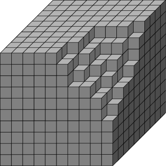
Figure 11: A melting crystal. The melting starts at the one corner of the crystal. Each cube is possibly removed (melt) only if its three faces do not touch the other cubes. Each removed cube contributes the factor $q=e^{-\mu/T}$ ($\mu>0$, $T>0$) to the weight of the configuration.

Figure 12: The stacked cubes corresponding to Figure 11. The configurations are in one-to-one correspondence with plane partitions. The above configuration is described by a configuration of the plane partition $|\pi|=58$.

Definition 6.1.

A plane partition $\pi$ is a two-dimensional array of non-negative integers $\pi_{ij}$ ($i,j>0$) satisfying $\pi_{ij}\geq\pi_{i+1\,j}$, $\pi_{ij}\geq\pi_{i\,j+1}$.

The plane partitions can be regarded as a three-dimensional generalization of the Young diagram. In this three-dimensional diagram, $\pi_{ij}$ corresponds to the height of stacked cubes on the coordinate $(i,j)$. Then the total number of the stacked cubes is given by $|\pi|:=\sum_{i,j\geq 1}\pi_{ij}$. For later convenience, let us describe some properties satisfying the diagonal slices of $\pi$, which is defined as follows.

Definition 6.2.

For a plane partition $\pi$, the $m$th ($m\in\mathbb{Z}$) diagonal slice $\pi^{(m)}$ is a sequence whose elements are defined as

$$\pi^{(m)}_{j}=\pi_{j-m\,\,j}\quad\text{for $j>\max(0,m)$}.$$ (6.1)

First, each diagonal slice $\pi^{(m)}$ is a partition, i.e., a sequence of weakly decreasing non-negative integers. Second, theses partitions satisfy the following interlacing property.

Lemma 6.3.

The series of partitions $\pi^{(m)}$ satisfies the interlacing relation

$$\cdots\pi^{(-2)}\prec\pi^{(-1)}\prec\pi^{(0)}\succ\pi^{(1)}\succ\pi^{(2)}\cdots.$$ (6.2)

See Figure 13 for an example of the diagonal slices.

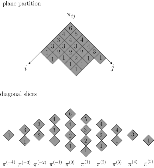
Figure 13: The diagonal slices of the plane partition $\pi$ defined in Figure 12.

The partition function $Z$ of the system of the melting crystal is regarded as the generating function of the plane partition, and is known to be given by the so-called MacMahon function [22]:

$$Z=\sum_{\pi}q^{|\pi|}=\prod_{n=1}^{\infty}\frac{1}{(1-q^{n})^{n}}\quad(0<q<1).$$ (6.3)

Now we consider the case that a plane partition $\pi$ is contained in a certain finite box of size, say $N_{1}\times N_{2}\times L$. Let us call such a partition the boxed plane partition and write it as $\pi\subseteq[N_{1},N_{2},L]$. For this boxed plane partition, the following is valid:

$$\pi^{(-N_{1})}=\pi^{(N_{2})}=\emptyset,\quad\pi_{i\,N_{2}+1}=\pi_{N_{1}+1\,j}=0\,\,\,(i,j\geq 1),$$ (6.4)

and hence the interlacing relation (6.2) is restricted to

$$\emptyset=\pi^{(-N_{1})}\prec\cdots\prec\pi^{(-1)}\prec\pi^{(0)}\succ\pi^{(1)}\succ\cdots\succ\pi^{(N_{2})}=\emptyset.$$ (6.5)

This case corresponds to a system of the melting rectangular crystal of size $N_{1}\times N_{2}\times L$. Then the partition function of the system is given by [22]:

$$Z_{\rm box}=\sum_{\pi\subseteq[N_{1},N_{2},L]}q^{|\pi|}=\prod_{j=1}^{N_{1}}\prod_{k=1}^{N_{2}}\frac{1-q^{L+j+k-1}}{1-q^{j+k-1}}.$$ (6.6)

In the limit $q\to 1$, this formula gives the number of the plane partitions contained in the box $N_{1}\times N_{2}\times L$. In [2], the formula (6.6) for the box $N\times N\times L$ is reproduced by utilizing the scalar products of the phase model.

Inspired by that work, we extend the method to the case for the non-Hermitian phase model and calculate the partition function for the statistical mechanical model of a melting crystal with the size $N\times N\times L$. The partition function of the model is defined as

$$Z_{\rm box}(\beta)=\sum_{\pi\subseteq[N,N,L]}\Phi(q,\beta;\pi)q^{|\pi|}\quad(0<q<1),$$

$$\Phi(q,\beta;\pi)=\prod_{j=1}^{N}\prod_{k=1}^{N-j}\left[(1+\beta q^{j})^{-\delta(\pi_{k}^{(j)},\,\pi_{k+1}^{(j-1)})}(1+\beta q^{1-j})^{1-\delta(\pi_{k}^{(-j)},\,\pi_{k}^{(1-j)})}\right],$$ (6.7)

where $\delta(i,j)$ denotes the Kronecker delta: $\delta(i,j)=\delta_{i\,j}$. Here we comment on the physical meaning of the additional potential factor $\Phi(q,\beta;\pi)$. This factor can be interpreted to reflect, such as microscopic interactions among atoms. For $\beta>0$, it brings out a surface flattening effect in the region $j>i$ in Figure 12 or 13. In contrast to this, in the region $j<i$, the potential causes a surface roughening effect. The strength of the effects decreases (resp. increases) with distance from the plane $i=j$ in the region $j>i$ (resp. $i<j$).

On the other hand, for $\beta<0$, the potential structure is much more complicated. (i) For $\beta<-2$, the potential $\Phi(q,\beta;\pi)$ denotes a roughening effect in $i<j<\log(-2/\beta)/\log(q)\cup j<i$, and a flattening effect in the other region. (ii) For $-2\leq\beta<0$, it denotes a roughening effect in $1-\log(-2/\beta)/\log q<j<i$, and a flattening effect in the other region. Note that for $\beta<0$, the model sometimes becomes physically ill-defined, because $\Phi(q,\beta;\pi)$ possibly takes negative values.

In any cases, due to the strength of the force is not symmetric with respect to the plane $i=j$, the expected shape of the melting crystal is not symmetric with respect to $i=j$ except for $\beta=0$.

The partition function $Z_{\rm box}(\beta)$ is explicitly evaluated by using the Cauchy identity (2.13) and Corollary 3.13. The following and subsequent Corollaries are the main results of this section.

Corollary 6.4.

The partition function $Z_{\rm box}(\beta)$ is given by

$$Z_{\rm box}(\beta) =\frac{q^{N(N-1)/2}\prod_{j=1}^{N}(1+\beta q^{j})^{j-1}}{\prod_{1\leq j<k\leq N}(q^{j}-q^{k})^{2}}\mathrm{det}_{N}\left[\frac{1-q^{(j+k-1)(L+N)}\left(\frac{1+\beta q^{1-k}}{1+\beta q^{j}}\right)^{N-1}}{1-q^{j+k-1}}\right].$$ (6.8)

Proof.

Consider the Cauchy identity given by (2.13) for $\lambda=\pi^{(0)}$. Then applying Corollary 3.13, the Grothendieck polynomials in the left hand side are given by

$$G_{\pi^{(0)}}(z_{1},\dots,z_{N};\beta)=\sum_{\pi^{(0)}\succ\dots\succ\pi^{(N)}=\emptyset}\prod_{l=1}^{N}z_{l}^{|\pi^{(l-1)}|-|\pi^{(l)}|}\prod_{j=1}^{N}\prod_{k=1}^{N-j}\left[1+\beta z_{j}-\beta z_{j}\delta_{\pi_{k+1}^{(j-1)}\,\pi_{k}^{(j)}}\right],$$

$$G_{\pi^{(0)\vee}}(w_{1},\dots,w_{N};\beta)=\sum_{\emptyset=\pi^{(-N)\vee}\prec\dots\prec\pi^{(0)\vee}}\prod_{l=1}^{N}w_{l}^{L+|\pi^{(-l)}|-|\pi^{(1-l)}|}$$

$$\qquad\qquad\qquad\qquad\qquad\quad\times\prod_{j=1}^{N}\prod_{k=1}^{N-j}\left[1+\beta w_{j}-\beta w_{j}\delta_{\pi_{k}^{(1-j)}\,\pi_{k}^{(-j)}}\right].$$ (6.9)

Here we have used $\pi^{(j)\vee}_{k}=L-\pi^{(j)}_{N-|j|-k+1}$ and the properties (3.4), (6.4) and (6.5) for the explicit evaluations. The insertion of them into the Cauchy identity (2.13) yields

$$\sum_{\pi\subseteq[N,N,L]}\prod_{j=1}^{N}z_{j}^{|\pi^{(j-1)}|-|\pi^{(j)}|}w_{j}^{|\pi^{(-j)}|-|\pi^{(1-j)}|}$$

$$\quad\qquad\quad\times\prod_{j=1}^{N}\prod_{k=1}^{N-j}\left[(1+\beta z_{j})^{-\delta(\pi_{k}^{(j)}\,,\pi_{k+1}^{(j-1)})}(1+\beta w_{j})^{1-\delta(\pi_{k}^{(-j)}\,,\pi_{k}^{(1-j)})}\right]$$

$$\quad=\frac{\prod_{j=1}^{N}(1+\beta z_{j})^{j-1}}{\prod_{1\leq j<k\leq N}(z_{j}-z_{k})(w_{j}^{-1}-w_{k}^{-1})}\mathrm{det}_{N}\left[\frac{1-(z_{j}w_{k}^{-1})^{L+N}\left(\frac{1+\beta w_{k}}{1+\beta z_{j}}\right)^{N-1}}{1-z_{j}w_{k}^{-1}}\right].$$ (6.10)

Setting $z_{j}=q^{j}$ and $w_{j}=q^{1-j}$ in the above, we finally arrive at (6.6). ∎

Set $\beta=0$ in (6.8), then the formula (6.6) is reproduced. Moreover taking the limit $L\to\infty$ and $N\to\infty$ we have the following generalized MacMahon function which reduces to the ordinary MacMahon function (6.3) for $\beta=0$ and Euler’s generating function at $\beta=-1$.

Corollary 6.5.

The partition function (6.8) in the limit $L\to\infty$ and $N\to\infty$ is given by

$$Z(\beta):=\lim_{L,N\to\infty}Z_{\rm box}(\beta)=\prod_{n=1}^{\infty}\frac{(1+\beta q^{n})^{n-1}}{(1-q^{n})^{n}},$$ (6.11)

which becomes the MacMahon function and Euler’s generating function at $\beta=0$ and $\beta=-1$ respectively.

For $\beta=0$, the partition function $Z(0)$ is nothing but the MacMahon function (6.6) which is a generating function of the plane partitions. And surprisingly, for $\beta=-1$ which corresponds to the TASEP (resp. TAZRP) in the language of the five-vertex model (resp. the non-Hermitian phase model), $Z(-1)$ is nothing but a generating function for the numbers of possible partitions of natural numbers which is due to Euler:

$$Z(-1)=\prod_{n=1}^{\infty}\frac{1}{1-q^{n}}=\sum_{\lambda}q^{|\lambda|}.$$ (6.12)

The expression for the partition function (6.11) means that the melting crystal model we introduced unifies the generating functions of the two-dimensional and three-dimensional Young diagrams (6.11). The enumeration problems for two-dimensional Young diagrams can be treated by the three-dimensional melting crystal model at the point $\beta=-1$. Note that there are other melting crystal models based on the Macdonald polynomials [25, 26], whose partition functions are different but have simple expressions in the infinite volume limit as ours, including the MacMahon function at a special point. But if one wants to relate the results in [25, 26] with the Euler’s generating function, one has to multiply infinite products. This means that one should multiply infinite products to the weights assigned to each plane partition, which seems to be an artificial operation, unnatural from the point of view of enumeration.

Note here that the partition function (6.11) is physically well-defined for $\beta\geq-1$ which is a condition for positivity of $Z(\beta)$. The entropy $S(\beta)$ for the model (6.11) can be calculated by using the relation $Z(\beta)=e^{S(\beta)-E/T}$, where $E:=T^{2}{\partial}^{2}\log Z(\beta)/{\partial}T^{2}$ is the internal energy. Explicitly it reads

$$S(\beta)=\sum_{n=1}^{\infty}\frac{\mu n}{T}\left[\frac{\beta(n-1)}{\beta+q^{-n}}+\frac{n}{q^{-n}-1}\right]+\sum_{n=1}^{\infty}\log\left[\frac{(1+\beta q^{n})^{n-1}}{(1-q^{n})^{n}}\right]\quad(\beta\geq-1),$$ (6.13)

where $q=e^{-\mu/T}$ $(\mu>0,T>0)$. From this expression, it can be easily followed that the entropy $S(\beta)$ is a monotonically increasing function of $\beta$. In Figure 14, the temperature dependence of the entropy is depicted for various values of $\beta$.

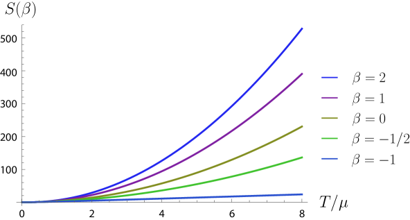
Figure 14: The temperature dependence of the entropy $S(\beta)$ (6.13) is depicted for various values of $\beta$.

7 Conclusion

In this paper, we studied the non-Hermitian phase model and showed that the wavefunctions is nothing but the Grothendieck polynomials. To show this, we reviewed the integrable five-vertex model, and introduced the skew Grothendieck polynomials for a single variable as matrix elements of a $B$-operator. The addition theorem for the Grothendieck polynomials follows from the equivalence between the wavefunctions of the five-vertex model and the Grothendieck polynomials. Showing that the matrix element of the $B$-operator in the non-Hermitian phase model is given by the skew Grothendieck polynomials, and then applying the addition theorem, we derive the wavefunctions of the non-Hermitian phase model, which can also be expressed by the Grothendieck polynomials. Our works establish the $K$-theoretic boson-fermion correspondence at the level of wavefunctions.

As another application of the boson-fermion correspondence, we discussed the statistical mechanical model of a three-dimensional melting crystal and exactly derive the partition functions, which is interpreted as a $K$-theoretic generalization of the MacMahon function. Surprisingly, the $K$-theoretic MacMahon function includes not only the generating function of the plane partitions but also Euler’s generating function of the partitions. Our refinement of the melting crystal model unifies the treatment of the enumeration problems of two-dimensional and three-dimensional Young diagrams. The reason why two-dimensional objects appear for $K$-theory is not known now, and its geometric meaning deserves to be investigated in the future.

The hermitian phase model is described by the Schur polynomials. Since the determinant representations of the scalar products are essentially the Cauchy identity for the Schur polynomials, it has connections with KP equation and the Toda lattice [26, 27, 28]. It is interesting to examine whether this classical integrable interpretation can be lifted to the case of the integrable five-vertex model and the non-Hermitian phase model, by making connection with the existing classical integrable system or extending to some extent.

In the words of geometry, our works on the relation between non-Hermitian integrable models and Grothendieck polynomials mean that non-Hermitian integrable models provide a natural framework to study the quantum $K$-theory of Grassmannian varieties. For the hermitian phase model, the quantum cohomology ring and the Verlinde ring are shown to be described by the ring defined by the model under the quasiperiodic boundary condition [4], where the Bethe ansatz equation plays the role of the ideal. We would like to make further investigations on quantum $K$-theoretic objects in our framework in the future.

One of the problems we are planning to investigate is to lift the relation between integrable models and $K$-theoretic objects to other types of Grassmannian varieties. There are several extensions and variations of the Schur polynomials. The Schur $P$, Schur $Q$, Jack, Hall-Littlewood and the Macdonald polynomials have connections with the $q$-boson model [6, 29, 30]. On the other hand, the $K$-theoretic extension of the Schur $P$ and Schur $Q$ polynomials are introduced in [13]. We expect to find connections between these $K$-theoretical symmetric polynomials and the integrable models such as the non-Hermitian $q$-boson model [31, 32, 33], for example.

Appendix

In this Appendix, we show the $L$-operator of the five-vertex model (2.2) is a particular reduction of a more general six-vertex model. We start from the $R$-matrix of the following six-vertex model satisfying the Yang-Baxter relation (2.5)

$$R(u,v) =\begin{pmatrix}f(v,u;t)&0&0&0\\ 0&t&g(v,u;t)&0\\ 0&g(v,u;t)&1&0\\ 0&0&0&f(v,u;t)\end{pmatrix},$$

$$f(v,u;t) =\frac{u^{2}-tv^{2}}{u^{2}-v^{2}},\,g(v,u;t)=\frac{(1-t)uv}{u^{2}-v^{2}},$$

including the $R$-matrix of the five-vertex model (2.4) as a special point $t=0$. One can show that the following $L$-operator solves the $RLL$ relation (2.3) for this $R$-matrix of the six-vertex model

$$L(u)=\begin{pmatrix}\alpha_{3}u+\alpha_{4}u^{-1}&0&0&0\\ 0&\alpha_{3}tu+\alpha_{4}u^{-1}&(1-t)\alpha_{1}&0\\ 0&(1-t)\alpha_{2}&\alpha_{5}u+\alpha_{6}u^{-1}&0\\ 0&0&0&\alpha_{5}u+\alpha_{6}tu\end{pmatrix},$$

where the parameters $\alpha_{j},\ j=1,\cdots,6$ and $t$ satisfy the relations

$$(1-t)\alpha_{1}\alpha_{2}+\alpha_{3}\alpha_{6}-\alpha_{4}\alpha_{5}=0,$$

$$(t^{2}-t)\alpha_{1}\alpha_{2}+t^{2}\alpha_{3}\alpha_{6}-\alpha_{4}\alpha_{5}=0.$$

The $R$-matrix of the six-vertex model is recovered from the $L$-operator by the choice of the parameters $\alpha_{1}=\alpha_{2}=\alpha_{3}=\alpha_{5}=1,\ \alpha_{6}=-1,\ \alpha_{4}=-t$.

Another particular choice of the $L$-operator of the general six-vertex model $t=\alpha_{4}=0,\ \alpha_{1}=\alpha_{2}=\alpha_{3}=1,\ \alpha_{6}=-1,\ \alpha_{5}=-\beta^{-1}$ gives the $L$-operator for the five-vertex model (2.2), whose wavefunction are the Grothendieck polynomials.

References

[1]
E. Date, M. Jimbo, M. Kashiwara and T. Miwa,
Transformation groups for soliton equations, in:
Nonlinear Integrable Systems-Classical Theory and
Quantum Theory (ed. by M. Jimbo and T. Miwa),
World Scientific, Singapore 1983, 39-119.
[2]
N.M. Bogoliubov,
Boxed plane partitions as an exactly solvable boson model,
J. Phys. A 38 (2005) 9415-9430.
[arXiv:cond-mat/0503748v1]
[3]
K. Shigechi and M. Uchiyama,
Boxed skew plane partition and integrable phase model,
J. Phys. A 38 (2005) 10287-10306.
[arXiv:cond-mat/0508090v2]
[4]
C. Korff and C. Stroppel,
The -WZNW fusion ring: a combinatorial construction
and a realization as a quotient of quantum cohomology,
Adv. in Math. 225 (2010) 200-268.
[arXiv:0909.2347v2]
[5]
B. Brubaker, D. Bump and S. Friedberg,
Schur polynomials and the Yang-Baxter equation,
Commun. Math. Phys. 308 (2011) 281-301.
[arXiv:0912.0911v3]
[6]
M. Wheeler,
Free fermions in classical and quantum integrable models,
PhD thesis,
Department of Mathematics and Statistics, University of Melbourne.
[arXiv:1110.6703v1]
[7]
S. Okuda and Y. Yoshida,
G/G gauged WZW model and Bethe Ansatz for the phase model,
JHEP 11 (2012) 146.
[arXiv:1209.3800v2]
[8]
A. Okounkov and N. Reshetikhin,
Correlation function of Schur process with application
to local geometry of a random 3-dimensional Young diagram,
J. Amer. Math. Soc. 16 (2003) 581-603.
[arXiv:math/0107056v3]
[9]
A. Okounkov, N. Reshetikhin and C. Vafa,
Quantum Calabi-Yau and classical crystals, in:
The unity of mathematics, Birkhäuser Boston, Boston, 2006
281-301.
[arXiv:hep-th/0309208v2]
[10]
K. Motegi and K. Sakai,
Vertex models, TASEP and Grothendieck polynomials,
J. Phys. A: Math. Theor. 46 (2013) 355201.
[arXiv:1305.3030v3]
[11]
A. Lascoux and M. Schützenberger,
Structure de Hopf de l’anneau de cohomologie et de
l’anneau de Grothendieck d’une variété de drapeaux,
C. R. Acad. Sci. Parix Sér. I Math
295 (1982) 629-633.
[12]
S. Fomin and A.N. Kirillov,