Electron events from the scattering with solar neutrinos in the search of keV scale sterile neutrino dark matter

Abstract

In a previous work we showed that keV scale sterile neutrino dark matter $\nu_{s}$ is possible to be detected in $\beta$ decay experiment using radioactive sources such as ³T or ¹⁰⁶Ru. The signals of this dark matter candidate are mono-energetic electrons produced in neutrino capture process $\nu_{s}+N^{\prime}\to N+e^{-}$. These electrons have energy greater than the maximum energy of the electrons produced in the associated decay process $N^{\prime}\to N+e^{-}+{\bar{\nu}}_{e}$. Hence, signal electron events are well beyond the end point of the $\beta$ decay spectrum and are not polluted by the $\beta$ decay process. Another possible background, which is a potential threat to the detection of $\nu_{s}$ dark matter, is the electron event produced by the scattering of solar neutrinos with electrons in target matter. In this article we study in detail this possible background and discuss its implication to the detection of keV scale sterile neutrino dark matter. In particular, bound state features of electrons in Ru atom are considered with care in the scattering process when the kinetic energy of the final electron is the same order of magnitude of the binding energy.

Introduction

Among many dark matter(DM) candidates, keV scale sterile neutrino warm DM is a very interesting possibility. It has several virtues. Among them include 1) it’s capable to smooth the structure of the universe at small scale and reduce the over-abundance of small scale structures observed in the simulation of cold DM scenarios structure ; 2) it provides a fermionic dark matter candidate with an appropriate mass scale which naturally avoids the cusp core in the halo density profile Cusp ; 3) it naturally gives a lifetime longer than the age of the universe and does not need to include by hand a discrete or global symmetry to guarantee the stability or long lifetime of the DM Liao ; Liao2 ; 4) it’s easy to get such a DM candidate in well motivated models such as the seesaw models ABS ; review2 which are the most popular models for explaining the tiny masses of active neutrinos.

Many aspects of this warm DM candidate, e.g. the production mechanism in the early universe DW ; ABS ; others ; blrv ; ST ; PK , the astrophysical and cosmological constraints, possible models and symmetries, etc., have been analyzed and considered  bhl ; bnrst ; bnr ; birs ; blrv2 ; bri ; sh ; LMN ; GT ; CDS ; RT model-independently or in special models. Among them, attention has been paid to the detection of this keV scale DM. It was realized that indirect detection of this DM background in the universe to a good sensitivity can be achieved in principle using satellite observation of mono-energetic X-rays produced in two-body decay of the DM: $\nu_{s}\to\nu+\gamma$. However this observation scheme requires large statistics which is not available in present scale satellite observation program indirect . Direct detection of this DM candidate in laboratory has also been investigated Liao ; Liao2 ; LX ; LX1 ; SV ; BS ; ak . Because of its small mass and weak interaction, some authors found it not possible to detect this DM candidate in laboratory LX1 ; BS ; ak ; SV .

In a previous work we proposed that keV scale $\nu_{s}$ DM can be detected using $\beta$ decay nuclei such as ³T and ¹⁰⁶Ru Liao . It was found that with a small mixing with electron neutrino $\nu_{e}$, $\nu_{s}$ can be captured by ³T and ¹⁰⁶Ru in process $\nu_{s}+N^{\prime}\to N+e^{-}$. The signals of $\nu_{s}$ DM are mono-energetic electrons with energy well beyond the end point of the $\beta$ decay spectrum. It was shown in Liao that the signal electrons produced in the $\nu_{s}$ capture process have kinetic energy $Q_{\beta}+m_{\nu_{s}}$ where $m_{\nu_{s}}$ is the mass of $\nu_{s}$. $Q_{\beta}$ is the decay energy of the decay process $N^{\prime}\to N+e^{-}+{\bar{\nu}}_{e}$. $Q_{\beta}$ equals to the maximal kinetic energy of electrons produced in the decay process, i.e. the kinetic energy at the end point of the decay spectrum. For ¹⁰⁶Ru, $Q_{\beta}=39.4$ keV. For ³T, $Q_{\beta}=18.59$ keV. So for $m_{\nu_{s}}=2-5$ keV, the signal electrons have kinetic energy around $20$ keV for ³T and around $40$ keV for ¹⁰⁶Ru respectively. We found that with reasonable amount of ³T and ¹⁰⁶Ru target we can get a few to tens signal electrons per year. Hence, we concluded that detection of keV scale sterile neutrino DM is possible using this detection scheme. This conclusion is of general significance and the detection scheme using $\beta$ decay nuclei can be applied to $\nu_{s}$ DM in different models. More details and general features of this detection scheme have been further analyzed in LX .

Two kinds of background electron events have also been discussed in  Liao . One type of background events are generated when radioactive nuclei ³T or ¹⁰⁶Ru capture solar electron neutrinos of energy around keV and produce final electrons in an energy range close to that of $\nu_{s}$ capture process. These electrons can mimick the signal electron of $\nu_{s}$ DM. Fortunately, this type of background is sufficiently small because solar neutrino flux at keV energy range is pretty small. Another possible background events are electrons kicked out by neutrinos in the scattering of solar neutrinos with electrons in target matter. This type of background should be discussed in detail, which however was not done in detail in Liao , for the following reasons: 1) solar neutrinos with higher energy can also participate in the scattering process and the total solar neutrino flux contributing to the background events is significantly higher than that for the first type background; 2) since signal electrons have energy of tens keV which is the same order of magnitude of the binding energy of the electrons in inner shell of ¹⁰⁶Ru atoms, the bound state feature of initial electrons in the scattering process should be taken into account at least for the scattering with electrons in inner shell of ¹⁰⁶Ru atoms.

In this article we will discuss in detail the scattering of neutrinos with bound state electrons. Attention will be paid to the scattering of neutrinos with electrons in inner shell of Ru atom and the events of final electrons with energy of tens keV. We will analyze the detailed energy distribution of the scattering of neutrinos with bound state electrons. We will discuss the dependence of the scattering process on the neutrino energy. We will analyze electron events caused by the scattering with solar neutrinos and the limitations for the detection of keV scale sterile neutrino DM. In the following we will first review the bound state feature of electrons in ¹⁰⁶Ru and discuss some general features of the scattering of neutrinos with bound electrons. Then we will come to detailed discussions of the scattering of neutrinos with electrons in ¹⁰⁶Ru. Finally, we will discuss the events of the scattering of solar neutrinos with bound state electrons and discuss the implication for DM detection.

Electrons in ¹⁰⁶Ru atoms and its interaction with neutrinos

In this section we briefly review features of bound electrons in ¹⁰⁶Ru atom and discuss some general features of the scattering of neutrinos with bound electrons. For reasons to be explained below, we will not discuss in detail the scattering with bound electrons in ³T atom.

As noted above, the signal electrons produced in $\nu_{s}$ DM capture process, $\nu_{s}+N^{\prime}\to N+e^{-}$, have kinetic energy $Q_{\beta}+m_{\nu_{s}}$. For a keV scale $\nu_{s}$ DM with a mass $2-5$ keV, the signal electrons have kinetic energy around $20$ keV for ³T and $40$ keV for ¹⁰⁶Ru separately.

The atomic number of the Ruthenium element is 44. In Table. 1 we list the electronic levels of the ground state configuration of neutral Ruthenium atom CRC and the corresponding binding energies obtained from X-ray data CRC ; X-ray-evaluation . One can see that electrons in $K$ and $L$ shells have binding energies greater than keV. When considering final electrons with energy round $40$ keV, one would expect that bound state features may give some effects to the scattering of neutrinos with electrons at these energy levels. We would also expect that the effect of the bound state features in the scattering with electrons in L shell should be weaker than that in the scattering with electrons in K shell.

Electronic level	$K$	$L_{I}$	$L_{II}$	$L_{III}$	$M_{I}$	$M_{II}$	$M_{III}$	$M_{IV}$	$M_{V}$	$N_{I}$	$N_{II}$	$N_{III}$	$N_{IV}$	$N_{V}$	$O_{I}$
State	$1s$	$2s$	$2p_{\frac{1}{2}}$	$2p_{\frac{3}{2}}$	$3s$	$3p_{\frac{1}{2}}$	$3p_{3\over 2}$	$3d_{3\over 2}$	$3d_{5\over 2}$	$4s$	$4p_{1\over 2}$	$4p_{3\over 2}$	$4d_{3\over 2}$	$4d_{5\over 2}$	$5s$
No. of electrons	2	2	2	4	2	2	4	4	6	2	2	4	4	3	1
Binding E(keV)	$22.1$	$3.22$	$2.97$	$2.84$	$0.59$	$0.48$	$0.46$	$0.28$	$0.28$	$0.075$	$0.043$	$0.043$	$0.002$	$0.002$

Table 1: Ground state configuration of neutral $Ru$ atom and the binding energy from X-ray experiment X-ray-evaluation ; CRC .

For the scattering with electrons in M, N and O shells in Ru atom, we expect that bound state features of these electrons should not give large correction to the neutrino-electron scattering of interests to us. As noted above, we would be interested in the events of electrons with energy around $40$ keV. As can be seen in Table 1, this energy is at least about two orders of magnitude larger than the binding energy of electrons in M, N and O shells. Detailed studies, to be given in the following, shows that even effects of the bound state feature of the electrons in L shell are not large in the energy range $\lower 3.01385pt\hbox{$\;\stackrel{{\scriptstyle\textstyle>}}{{\sim}}\;$}40$ keV. These studies support what we expect for the scattering with electrons in M, N and O shells.

For ³T, the binding energy is the famous $13.6$ eV. It is three orders of magnitude smaller than the kinetic energy of interests to us, say $\sim 20$ keV. Similar to the discussion above for the electrons in M, N and O shells of Ru atom, it’s natural to expect that bound state features of initial electron in ³T should not give significant effect to the neutrino-electron scattering process when discussing events with final electrons of an energy around $20$ keV.

To understand in detail the scattering of neutrino with bound electron in Ru atom we need the wavefunction of the bound electron. Neglecting relativistic corrections, interactions of non-relativistic electrons in an atom include interaction with the nucleus through a central force and the interaction with other electrons. The Hamiltonian for such a system can be written as

$${\cal H}=\sum_{i}\frac{{\hat{p}_{i}}^{2}}{2m_{e}}-\sum_{i}\frac{Ze^{2}}{r_{i}}+\sum_{i<j}\frac{e^{2}}{r_{ij}},$$ (1)

where ${\hat{p}}_{i}$ is the momentum operator of the $i$th electron, $r_{i}$ the radius of the $i$th electron, $r_{ij}$ the distance between $i$th electron and $j$th electron, $e$ the charge of electron, $Z$ the atomic number. It’s very difficult to solve states of electrons including all details of these interactions. Fortunately, one can take the approximation that the forces acted by all other electrons on a single electron can be approximated to be a mean central force and the state of a single electron can be solved using an effective Hamiltonian

$${\cal H}_{i}=\frac{{\hat{p}_{i}}^{2}}{2m_{e}}-\frac{Ze^{2}}{r_{i}}+V_{i}(r_{i}),$$ (2)

where $V_{i}$ arises from the interaction of $i$th electron with all other electrons. A further approximation one can use is that the effect of an electron in an outer shell on an electron in an inner shell can be taken small, since the distance between these electrons can be considered large compared to distances between electrons in inner shell.

For electron in K shell of Ru atom, the above approximation works well. According to the approximation described above, an electron in K shell is similar to an electron in the ground state of the hydrogen atom except that the atomic number is replaced by $Z=44$. Using this approximation, the binding energy of an electron in K shell is estimated to be $\varepsilon=m_{e}Z^{2}\alpha^{2}/2$ where $\alpha$ is the fine structure constant. Using this approximation for an electron in K shell of Ru atom, we find that $\varepsilon\approx 26.3$ keV which is consistent with the binding energy from X-ray data shown in Table 1. This convinces us that the wavefunction of an electron in K shell of Ru atom can be approximated as the one similar to the wavefunction of 1s state in hydrogen atom. In momentum space this wavefunction can be written as

$$\varphi_{1s}(p)=\frac{2\sqrt{2}}{\pi}\frac{a_{K}^{3/2}}{(p^{2}a_{K}^{2}+1)^{2}}.$$ (3)

It satisfies

$$\int~{}d^{3}p~{}|\varphi_{1s}(p)|^{2}=1.$$ (4)

Eq. (3) is normalized to give a kinetic energy $1/(2m_{e}a_{K}^{2})$ where $a_{K}$ is the effective radius of the electron in the state of K shell. The binding energy equals to the kinetic energy $\varepsilon_{K}=1/(2m_{e}a_{K}^{2})$, as a consequence of the Virial theorem. So $a_{K}$ can be determined using binding energy shown in Table 1. If using only the central force from the interaction with the nucleus one has $a_{K}=1/(m_{e}Z\alpha)$ and one can recover the previous estimate:$\varepsilon_{K}=m_{e}Z^{2}\alpha^{2}/2$.

For electrons in L shell of Ru atom, the above approximation seems also working well. The evidence is the quasi-degeneracy of binding energies of $L_{I}$, $L_{II}$ and $L_{III}$ states as shown in Table 1. One can see that the binding energies of these energy levels are almost the same. This suggests that the dynamical $SO(4)$ symmetry works well for electrons in these states and the mean potentials acted on these electrons should be close to a $1/r$ law. So the wavefunctions of electrons in L level can be approximated as that similar to the $2s$ and $2p$ wavefunctions in the hydrogen atom. In momentum space we write these wavefunctions as

$$\varphi_{2s}(p) =\frac{a_{L}^{3/2}}{\pi}\frac{p^{2}a_{L}^{2}-1/4}{(p^{2}a_{L}^{2}+1/4)^{3}},$$ (5)

$$\varphi_{2p0}(p) =-\frac{ia_{L}^{3/2}}{\pi}\frac{p_{z}a_{L}}{(p^{2}a_{L}^{2}+1/4)^{3}},$$ (6)

$$\varphi_{2p\pm 1}(p) =\frac{a_{L}^{3/2}}{\sqrt{2}\pi}\frac{(p_{x}\pm ip_{y})a_{L}}{(p^{2}a_{L}^{2}+1/4)^{3}},$$ (7)

where $2pi$($i=0,\pm 1$) refers to states with different projections of angular momentum onto z direction. These wavefunctions satisfy

$$\int~{}d^{3}p~{}|\varphi_{l}(p)|^{2}=1,~{}~{}\textrm{$l=2s,2p0,2p+1,2p-1$}.$$ (8)

They are normalized to give a kinetic energy $1/(2^{3}m_{e}a_{L}^{2})$. The binding energy equals to the kinetic energy $\varepsilon_{L}=1/(2^{3}m_{e}a_{L}^{2})$, as a consequence of the Virial theorem. So $a_{L}$ can be determined using binding energy shown in Table 1. For simplicity we use a universal $\varepsilon_{L}$ for all $2s$ and $2p$ states in definitions given in Eqs. (5), (6) and (7).

For electrons in M, N and O shells, the situation is a bit complicated. As can be seen in Table 1, there are no quasi-degeneracies of states in M, N and O shells. Fortunately, these states have much smaller binding energies than the states in K and L shells. In particular, their binding energies are about two orders of magnitude smaller than the energy range of the kinetic energy of scattered electrons, i.e. $\lower 3.01385pt\hbox{$\;\stackrel{{\scriptstyle\textstyle>}}{{\sim}}\;$}40$ keV, which is of interests to us. We would expect that the bound state features of electrons in these states should not alter the scattering process significantly and we should be able to approximate these electrons as at rest with the energy equals to the rest mass.

Scattering of neutrino with bound electrons in Ru atom

For the scattering of a neutrino with free electron at rest, the cross section is well known RPP :

$$\frac{d\sigma_{0}}{dE_{k}}=\frac{G_{F}^{2}m_{e}}{2\pi}\bigg{[}(g_{V}+g_{A})^{2}+(g_{V}-g_{A})^{2}(1-\frac{E_{k}}{E_{\nu}})^{2}-(g_{V}^{2}-g_{A}^{2})\frac{E_{k}m_{e}}{E_{\nu}^{2}}\bigg{]},$$ (9)

where $E_{\nu}$ is the energy of initial neutrino, $E_{k}$ the kinetic energy of scattered electron, $g_{V,A}$ are the vector and axial-vector coupling constants RPP . $g_{V}=-\frac{1}{2}+2\sin^{2}\theta_{W}$ and $g_{A}=-\frac{1}{2}$ for muon and tau neutrino. For electron neutrino $g_{V}=\frac{1}{2}+2\sin^{2}\theta_{W}$, $g_{A}=\frac{1}{2}$. $\theta_{W}$ is the weak mixing angle with $\sin^{2}\theta_{W}=0.231$. The kinetic energy of the scattered electron lies in the range

$$E_{k}\subset[0,E_{\nu}/(1+m_{e}/(2E_{\nu}))].$$ (10)

One can see in Eq. (9) that the differential cross section varies slowly with respect to $E_{k}$.

For the scattering of a neutrino with bound electron in Ru atom, the neutrino directly transfers energy and momentum to the electron. The neutrino neither affects the other parts of the atom nor is affected by the other parts of the atom. This is the exactly the case that the impulse approximation works PWIA . Furthermore, we can approximate the wavefunction of the scattered electron as the plane wave. This is because we would concentrate on the energy range, $\lower 3.01385pt\hbox{$\;\stackrel{{\scriptstyle\textstyle>}}{{\sim}}\;$}40$ keV, for the scattered electron. For kinetic energy larger than the binding energy one can take the plane wave approximation for the wavefunction of the scattered electrons PWIA .

The scattering of a neutrino with bound electrons should in principle be treated in a relativistic framework. This requirement would give rise to complication if taking into account relativistic wavefunction of electron in bound state. Fortunately, we can simplify the discussion by noticing that the electrons in Ru atoms can be considered non-relativistic, as can be seen in Table 1. Furthermore, the spin-orbit coupling is zero for electrons in K shell which have zero angular momentum and the energy shift due to the spin-orbit coupling to electrons in L shell should give negligible effect to our result for the events with scattered electrons of $E_{k}\lower 3.01385pt\hbox{$\;\stackrel{{\scriptstyle\textstyle>}}{{\sim}}\;$}40$ keV. So we can approximately take spin and angular momentum as independent variables, as in the case of non-relativistic quantum mechanics. In this approximation the total wavefunction of the bound electron can be approximated as a product of a spinor and a wavefunction in x or p coordinates:

$$\Psi({\vec{x}})=\psi\phi({\vec{x}}),~{}~{}\Phi({\vec{p}})=\psi\varphi({\vec{p}}),$$ (11)

where $\psi$ is a spinor and it equals to $(1,0,0,0)^{T}$ or $(0,1,0,0)^{T}$ in standard Dirac representation of spinor.

In this approximation, one can find that the cross section of the scattering of a neutrino with an electron in a particular state $l$ can be written as

$$\frac{d\sigma_{l}}{dE_{k}}=\int~{}d^{3}p_{B}~{}|\varphi_{l}({\vec{p}}_{B})|^{2}\frac{d\sigma_{{\vec{p}}_{B}}}{dE_{k}},$$ (12)

where $E_{k}$ is the kinetic energy of final electron, $\sigma_{{\vec{p}}_{B}}$ the cross section of the scattering of a neutrino with an electron of energy $E_{B}=m_{e}-\varepsilon$ and momentum ${\vec{p}}_{B}$. Eq. (12) says that the neutrino has a probability, $|\varphi_{l}({\vec{p}}_{B})|^{2}d^{3}p_{B}$, to scatter with an electron carrying momentum ${\vec{p}}_{B}$ and the cross section is a sum of contributions of the scattering with electrons carrying all possible ${\vec{p}}_{B}$.

The energy and momentum conservation conditions for $\sigma_{{\vec{p}}_{B}}$ are

$$E_{\nu}+E_{B}=E^{\prime}_{\nu}+E_{e},~{}~{}{\vec{p}}_{\nu}+{\vec{p}}_{B}={\vec{p}}_{\nu}^{\hskip 2.84544pt\prime}+{\vec{p}}_{E},$$ (13)

where $E_{B}$ is the energy of bound electron as given above, $E_{e}$ the energy of final electron, $E_{\nu}$ the energy of initial neutrino, $E^{\prime}_{\nu}$ the energy of final neutrino, ${\vec{p}}_{\nu}$ the momentum of initial neutrino, ${\vec{p}}_{\nu}^{\hskip 2.84544pt\prime}$ the momentum of final neutrino, ${\vec{p}}_{E}$ the momentum of final electron. Using Eq. (11) one can find that

$$\frac{d\sigma_{{\vec{p}}_{B}}}{dE_{k}}=\frac{G_{F}^{2}}{4\pi^{2}|{\vec{p}}_{\nu B}|}~{}\int_{0}^{2\pi}~{}d\phi~{}\frac{1}{2}\sum_{spin}|{\cal M}|^{2}$$ (14)

where ${\vec{p}}_{\nu B}={\vec{p}}_{\nu}+{\vec{p}}_{B}$, $\phi$ is the azimuthal angle of ${\vec{p}}_{E}$ with respect to the axis of ${\vec{p}}_{\nu B}$ and

$$\frac{1}{2}\sum_{spin}|{\cal M}|^{2}=(g_{V}+g_{A})^{2}p^{\prime}_{\nu}\cdot p_{E}+(g_{V}-g_{A})^{2}p_{\nu}\cdot p_{E}\frac{E^{\prime}_{\nu}}{E_{\nu}}-(g_{V}^{2}-g_{A}^{2})\frac{m_{e}}{E_{\nu}}p_{\nu}\cdot p^{\prime}_{\nu}.$$ (15)

$p_{\nu},p^{\prime}_{\nu},p_{E}$ are the four-momenta of initial neutrino, final neutrino and final electron respectively. In Eq. (15) an average over spin of the initial electron has been performed.

Using Eq. (13) one can find that

$$p^{\prime}_{\nu}\cdot p_{E}=\frac{1}{2}(E_{T}^{2}-|{\vec{p}}_{\nu B}|^{2}-m_{e}^{2}),$$ (16)

$$2{\vec{p}}_{\nu B}\cdot{\vec{p}}_{E}=|{\vec{p}}_{\nu B}|^{2}+|{\vec{p}}_{E}|^{2}-(E_{T}-E_{e})^{2}$$ (17)

where $E_{T}=E_{\nu}+E_{B}$ is the total energy of the scattering process. One can see that the projection of ${\vec{p}}_{E}$ onto the axis of ${\vec{p}}_{\nu B}$ is fixed by the energy-momentum conservation condition but the azimuthal angle $\phi$ is not fixed. Using Eq. (17) one can easily find that

$$\frac{1}{2\pi}~{}\int_{0}^{2\pi}~{}d\phi~{}{\vec{p}}_{E}={\vec{p}}_{\nu B}~{}S,$$ (18)

where

$$S=\frac{|{\vec{p}}_{\nu B}|^{2}+|{\vec{p}}_{E}|^{2}-(E_{T}-E_{e})^{2}}{2|{\vec{p}}_{\nu B}|^{2}}.$$ (19)

Using Eq. (18) one can find that

$$\frac{d\sigma_{{\vec{p}}_{B}}}{dE_{k}}=\frac{G_{F}^{2}}{2\pi|{\vec{p}}_{\nu B}|}\frac{1}{2}\sum_{spin}|{\tilde{M}}|^{2}$$ (20)

where

$$\frac{1}{2}\sum_{spin}|{\tilde{M}}|^{2} =\frac{1}{2}(g_{V}+g_{A})^{2}(E_{T}^{2}-|{\vec{p}}_{\nu B}|^{2}-m_{e}^{2})+(g_{V}-g_{A})^{2}(E_{\nu}E_{e}-{\vec{p}}_{\nu}\cdot{\vec{p}}_{\nu B}S)\frac{E^{\prime}_{\nu}}{E_{\nu}}$$ (21)

$$-(g_{V}^{2}-g_{A}^{2})\frac{m_{e}}{E_{\nu}}[E_{\nu}(E_{T}-E_{e})-{\vec{p}}_{\nu}\cdot{\vec{p}}_{\nu B}(1-S)].$$

For ${\vec{p}}_{B}=0$ and $E_{B}=m_{e}$ one can easily show that Eq. (20) recovers Eq. (9).

Using Eq. (13) one can find that the energies of final electron and final neutrino lie in the following range

$$E_{e} \subset\bigg{[}\frac{(E_{T}-|{\vec{p}}_{\nu B}|)^{2}+m_{e}^{2}}{2(E_{T}-|{\vec{p}}_{\nu B}|)},\frac{(E_{T}+|{\vec{p}}_{\nu B}|)^{2}+m_{e}^{2}}{2(E_{T}+|{\vec{p}}_{\nu B}|)}\bigg{]}$$ (22)

$$E^{\prime}_{\nu} \subset\bigg{[}\frac{E_{T}^{2}-|{\vec{p}}_{\nu B}|^{2}-m_{e}^{2}}{2(E_{T}+|{\vec{p}}_{\nu B}|)},\frac{E_{T}^{2}-|{\vec{p}}_{\nu B}|^{2}-m_{e}^{2}}{2(E_{T}-|{\vec{p}}_{\nu B}|)}\bigg{]}.$$ (23)

A number of comments are as follows:

A) From Eqs. (17), (22) and (23) one can read out that not all electrons with all possible ${\vec{p}}_{B}$ can contribute to the cross section. Some ${\vec{p}}_{B}$ range is forbidden due to kinematical constraint. ${\vec{p}}_{B}$ allowed to contribute to the scattering process should satisfy

$$E_{T}^{2}-|{\vec{p}}_{\nu B}|^{2}-m_{e}^{2}\geq 0.$$ (24)

If $E_{T}^{2}-m_{e}^{2}\leq 0$, no ${\vec{p}}_{B}$ range can contribute to the kinematically allowed range and the process is forbidden. This is just the threshold condition for the process to happen, i.e. $E_{\nu}>\varepsilon$.

B) From Eqs. (22) and (23) one can read out that the energy ranges of the final particles depend on $|{\vec{p}}_{\nu B}|$. The total width of the range of electron energy is

$$\Delta E_{e}=E_{e}|_{max}-E_{e}|_{min}=\frac{E_{T}^{2}-|{\vec{p}}_{\nu B}|^{2}-m_{e}^{2}}{E_{T}^{2}-|{\vec{p}}_{\nu B}|^{2}}|{\vec{p}}_{\nu B}|.$$ (25)

C) One can check in Eq. (22) that the minimum of the energy of final electron is larger than or equals to $m_{e}$. To allow the energy range to reach $m_{e}$ it requires

$$E_{T}-|{\vec{p}}_{\nu B}|=m_{e}.$$ (26)

This requires that ${\vec{p}}_{B}$ lies in a very narrow range. Hence, the differential cross section for $E_{k}\approx 0$ range is suppressed by a factor arising from the momentum distribution of ${\vec{p}}_{B}$: $|\varphi({\vec{p}}_{B})|^{2}\delta^{3}p_{B}$.

D) From Eq. (22) one can show that $E_{e}|_{\max}$ increases with $|{\vec{p}}_{\nu B}|$. Using Eq. (24) one can find out the maximum energy of final electron in the scattering process:

$$E_{e}\leq\frac{1}{2}\bigg{(}E_{T}+\sqrt{E_{T}^{2}-m_{e}^{2}}+\frac{m_{e}^{2}}{E_{T}+\sqrt{E_{T}^{2}-m_{e}^{2}}}\bigg{)}=E_{T}.$$ (27)

As a comparison, we can find in Eq. (10) that for the scattering with free electron at rest the maximum energy of final electron is $\frac{1}{2}[m_{e}+2E_{\nu}+m_{e}^{2}/(m_{e}+2E_{\nu})]$. For $E_{\nu}\gg\varepsilon$ we can easily figure out that the energy of final electron extends beyond the range allowed by the scattering with free electron at rest.

E) Eqs. (12) and (20) appear to be singular for $|{\vec{p}}_{\nu B}|\to 0$. This is an artificial singularity. As can be seen in Eq. (25), the energy range of final electron shrinks also as $|{\vec{p}}_{\nu B}|\to 0$. This cancels the singular term in Eqs. (12) and (20) in the integrated cross-section. Furthermore, one can see that $|{\vec{p}}_{\nu B}|\approx 0$ corresponds to a very narrow range of ${\vec{p}}_{B}$. In numerical calculation, the contribution to differential cross section of electrons in this narrow range can be easily controlled by taking it as $|\varphi({\vec{p}}_{B})|^{2}~{}\delta^{3}p_{B}~{}\Delta E_{e}/|{\vec{p}}_{\nu B}|~{}\frac{1}{2}G_{F}^{2}|{\tilde{M}}|^{2}/(2\pi)$. Using Eq. (25), one can see that it is suppressed by the factor $|\varphi({\vec{p}}_{B})|^{2}~{}\delta^{3}p_{B}$ and in practice one can neglect it by taking a small enough range of $\delta^{3}p_{B}$.

Numerical result and discussion

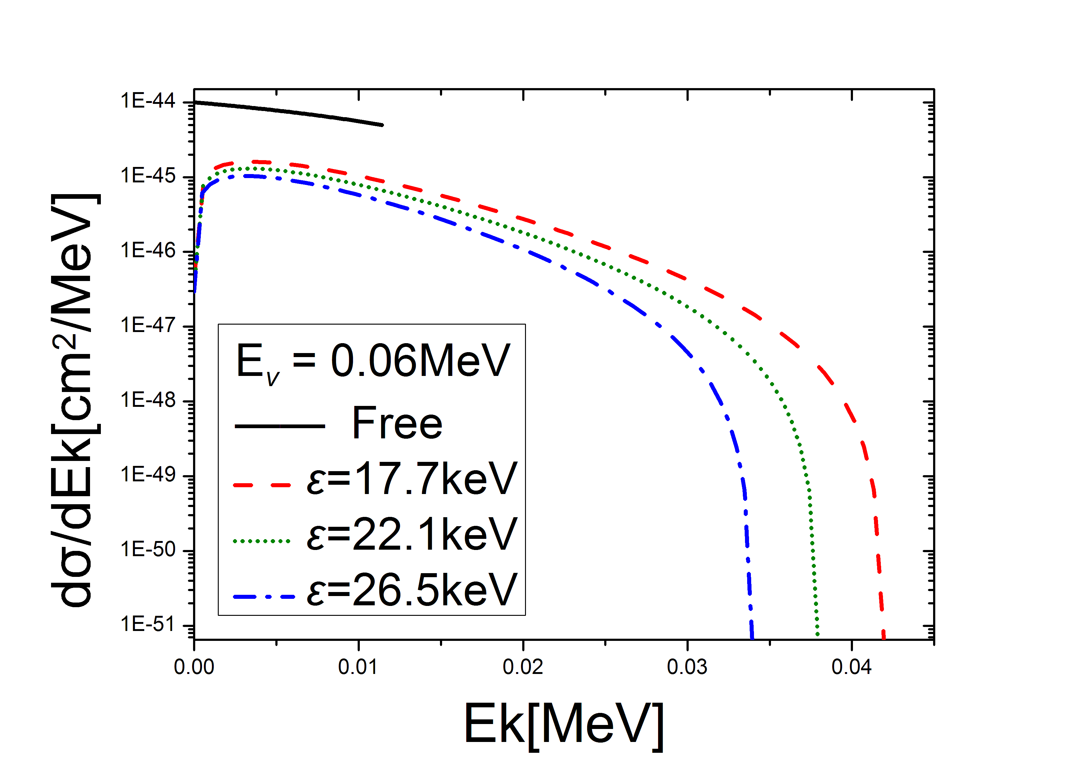
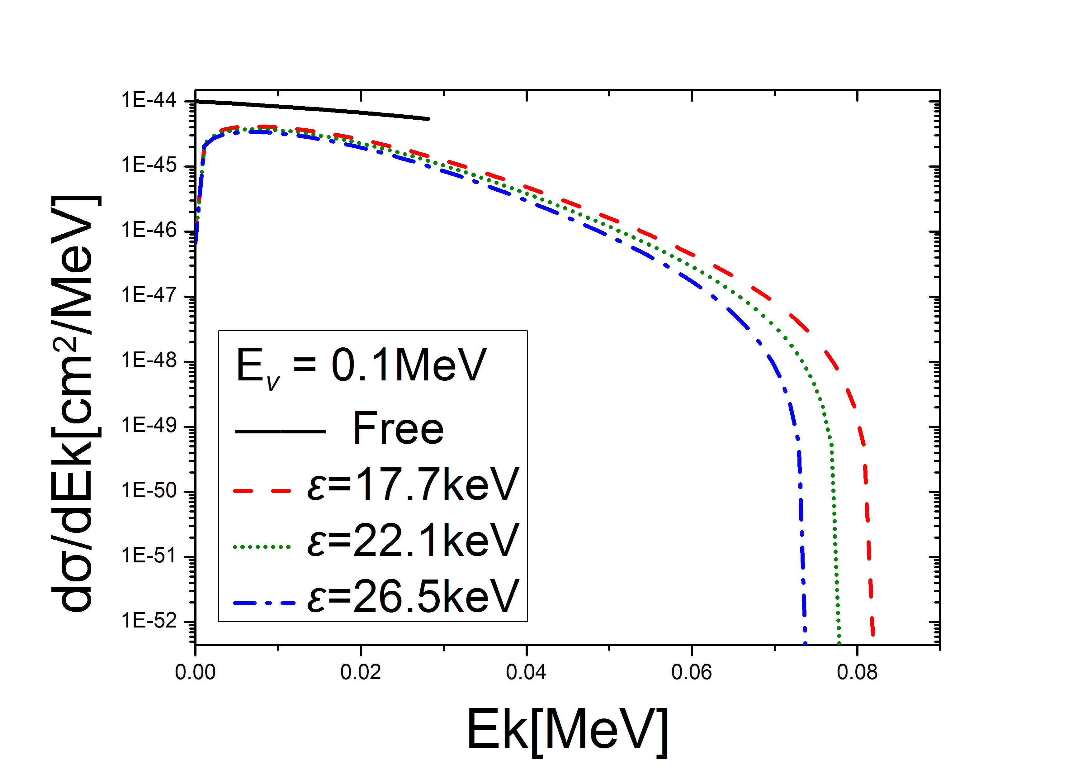
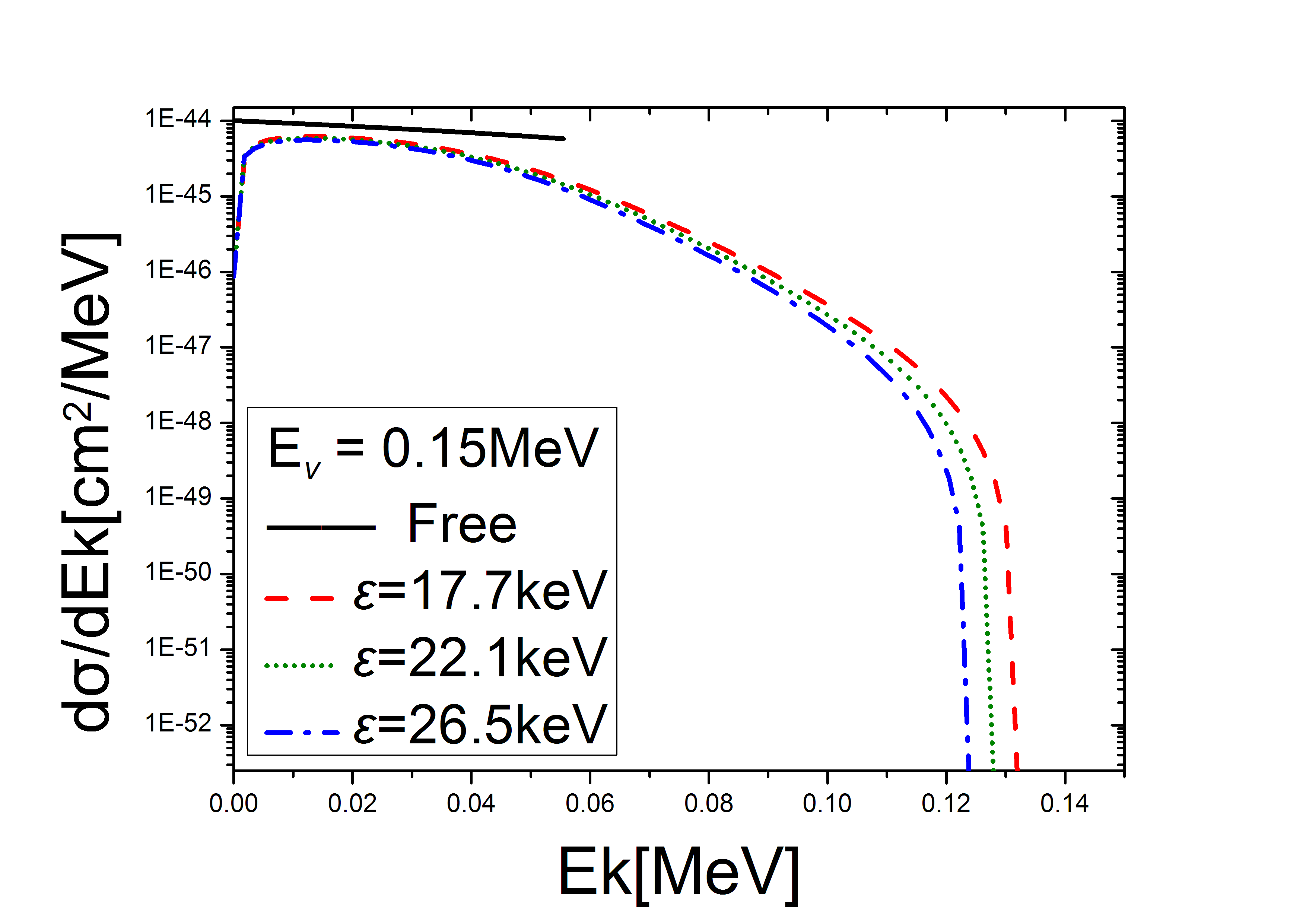
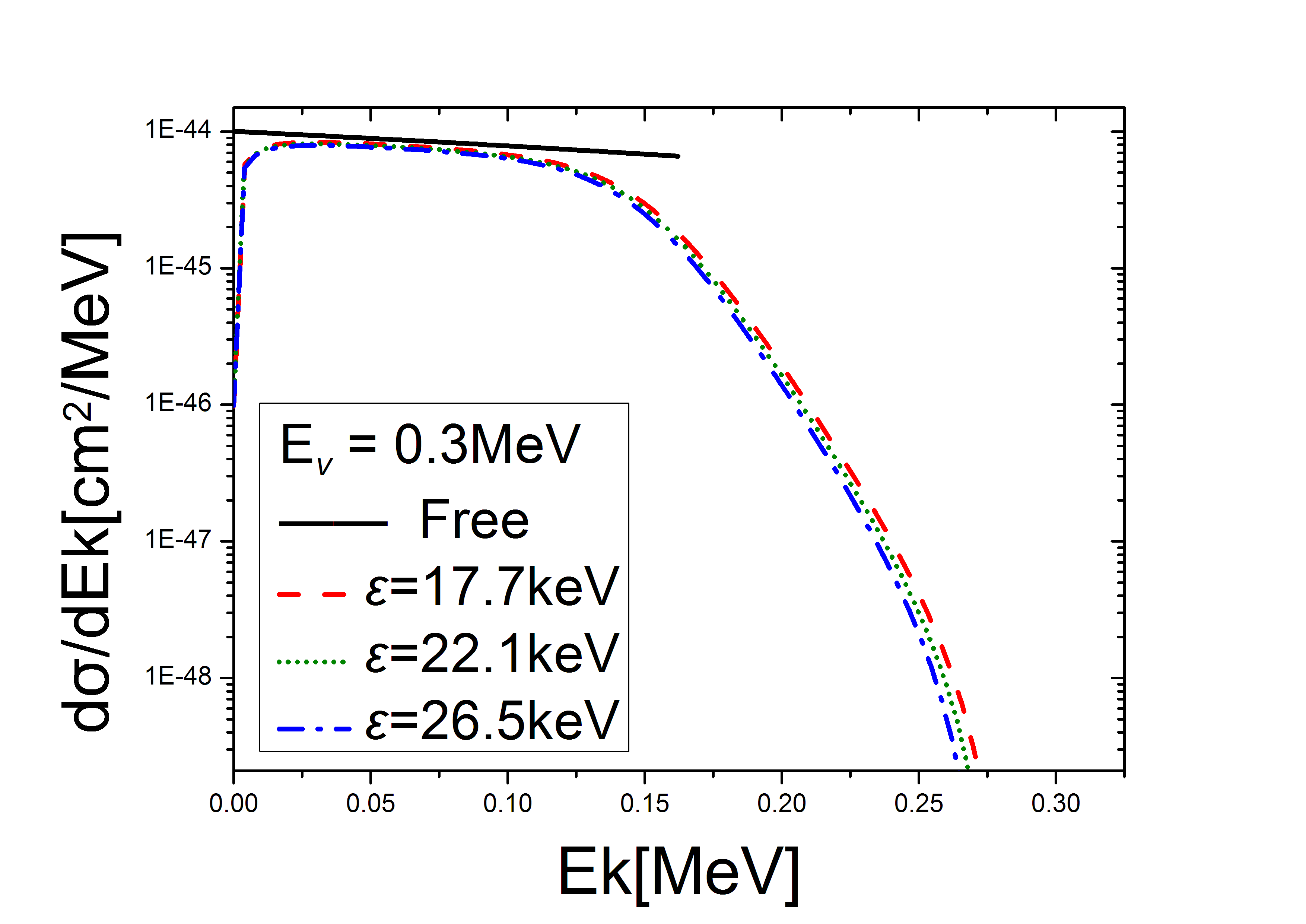
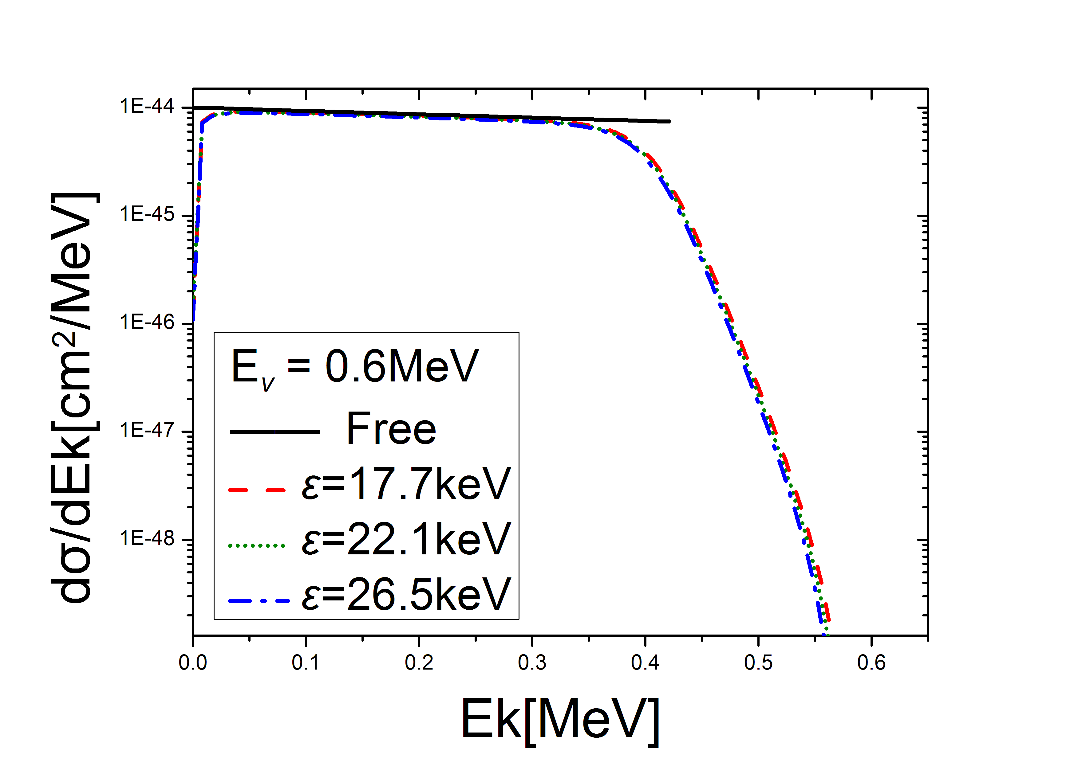
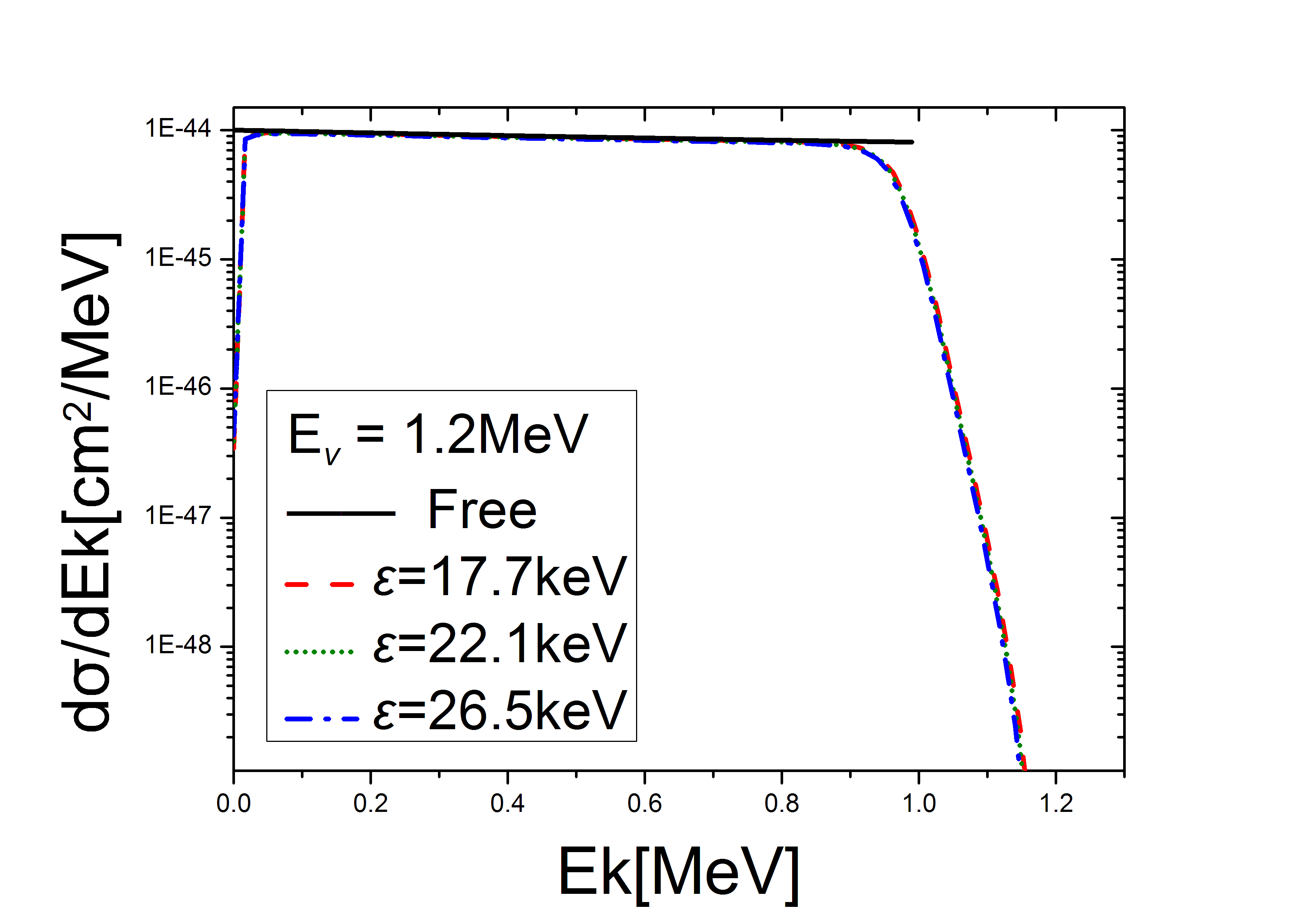
Figure 1: Differential cross section of the scattering of an electron neutrino with bound electron in K shell of Ru atom. The black solid line is for the scattering with electron at rest with $E_{k}$ in the kinematically allowed range $[0,E_{\nu}/(1+m_{e}/(2E_{\nu}))]$. Three colored lines are for $\varepsilon=17.7,22.1,26.5$ keV respectively.

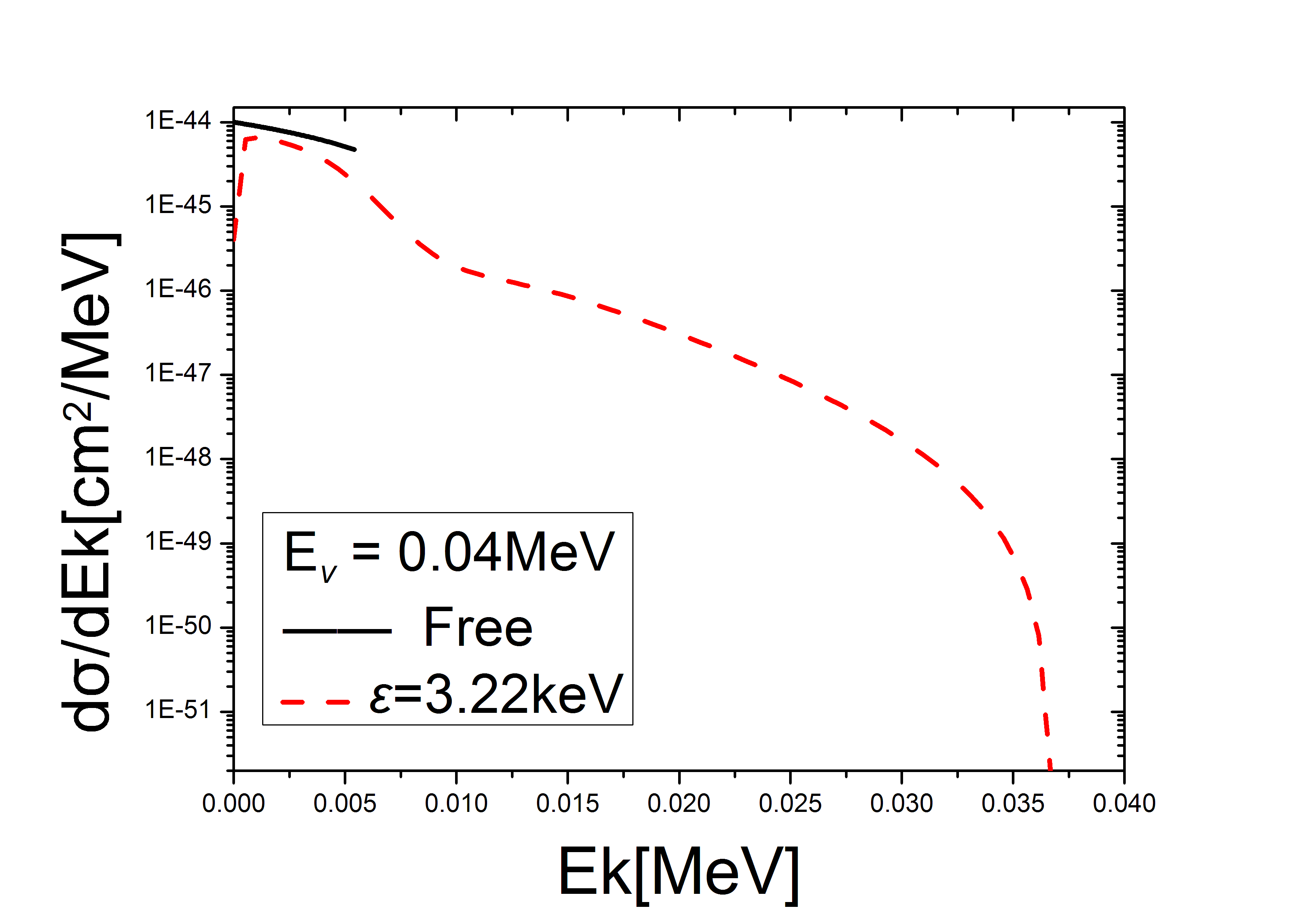
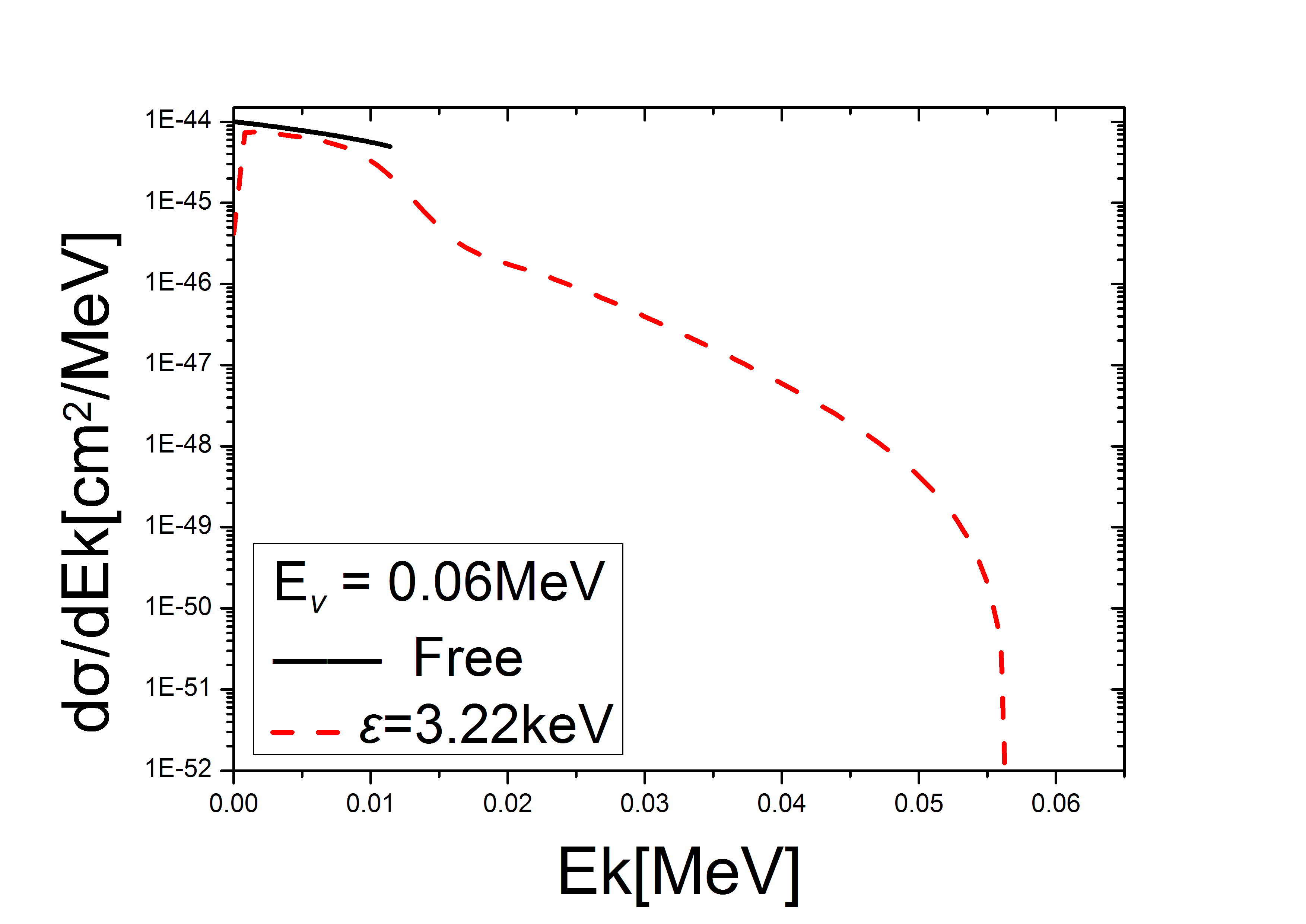
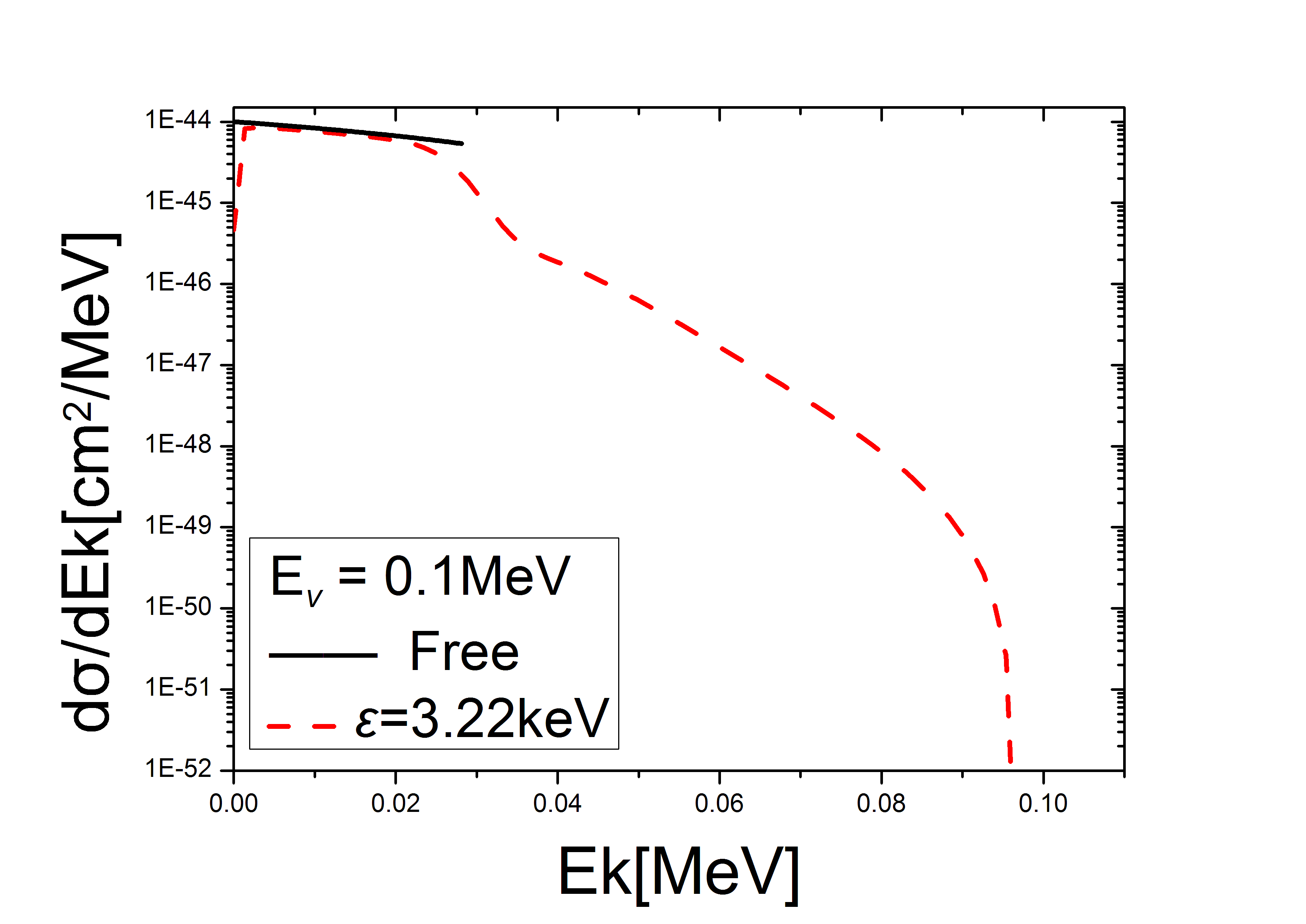
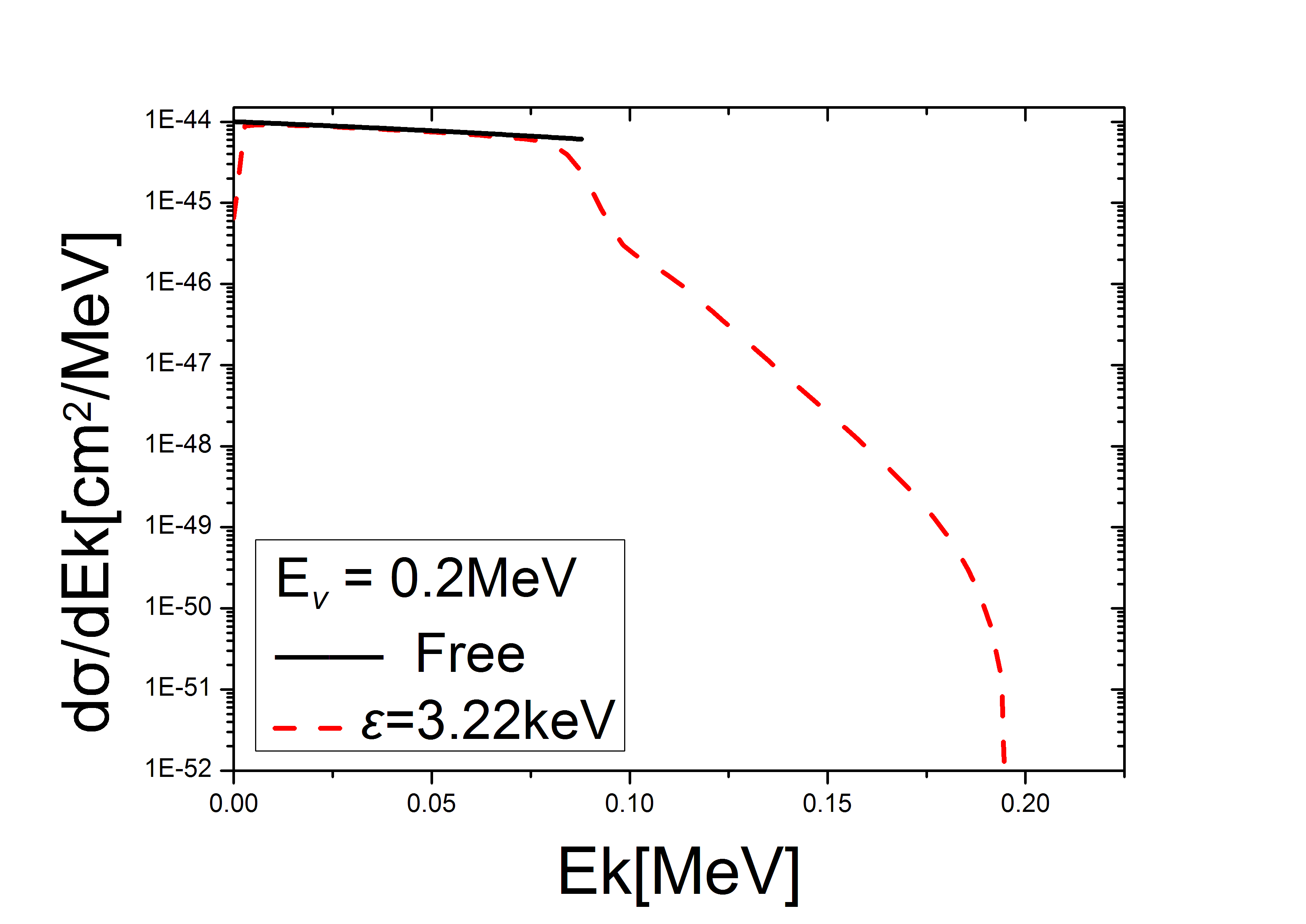
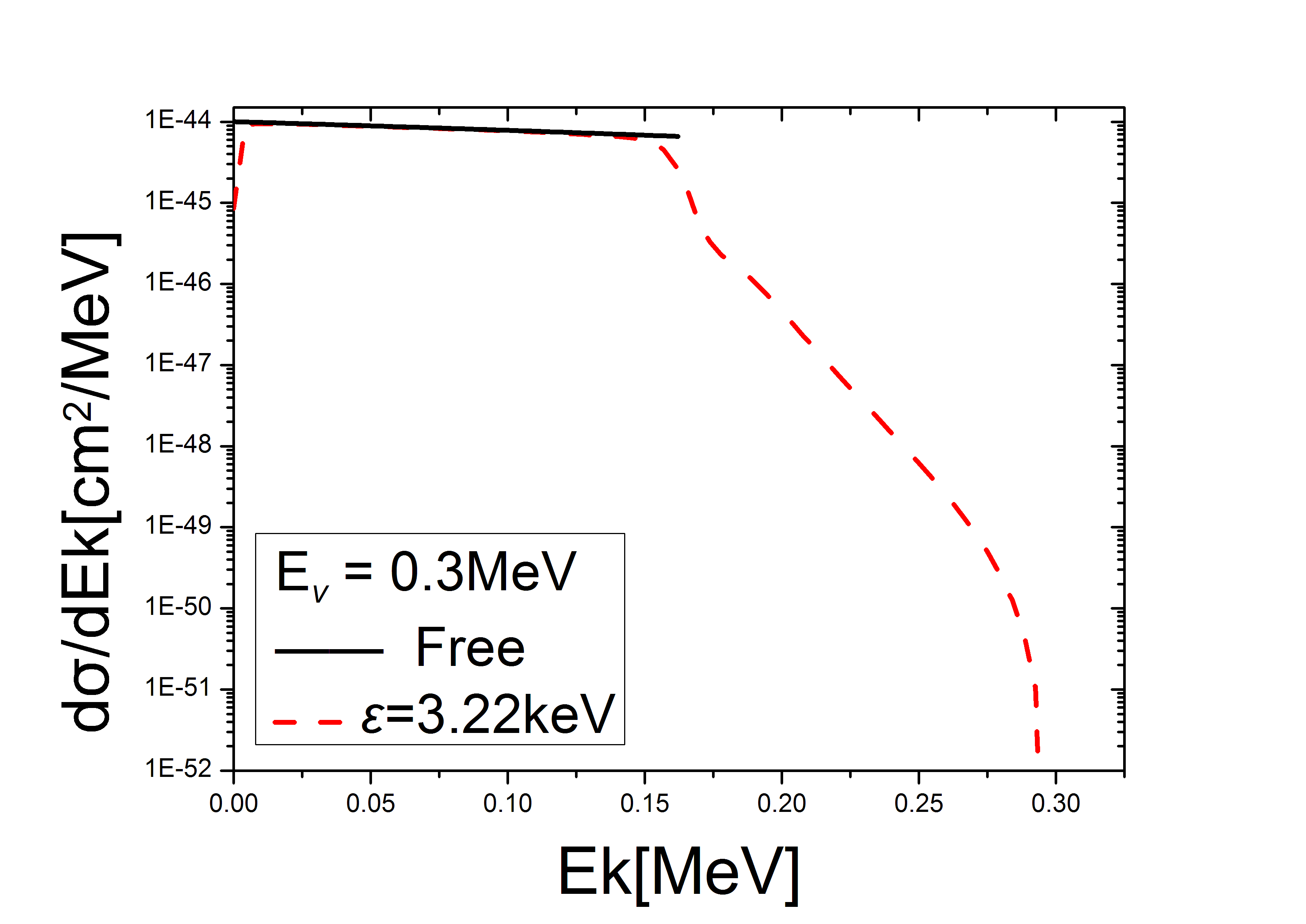
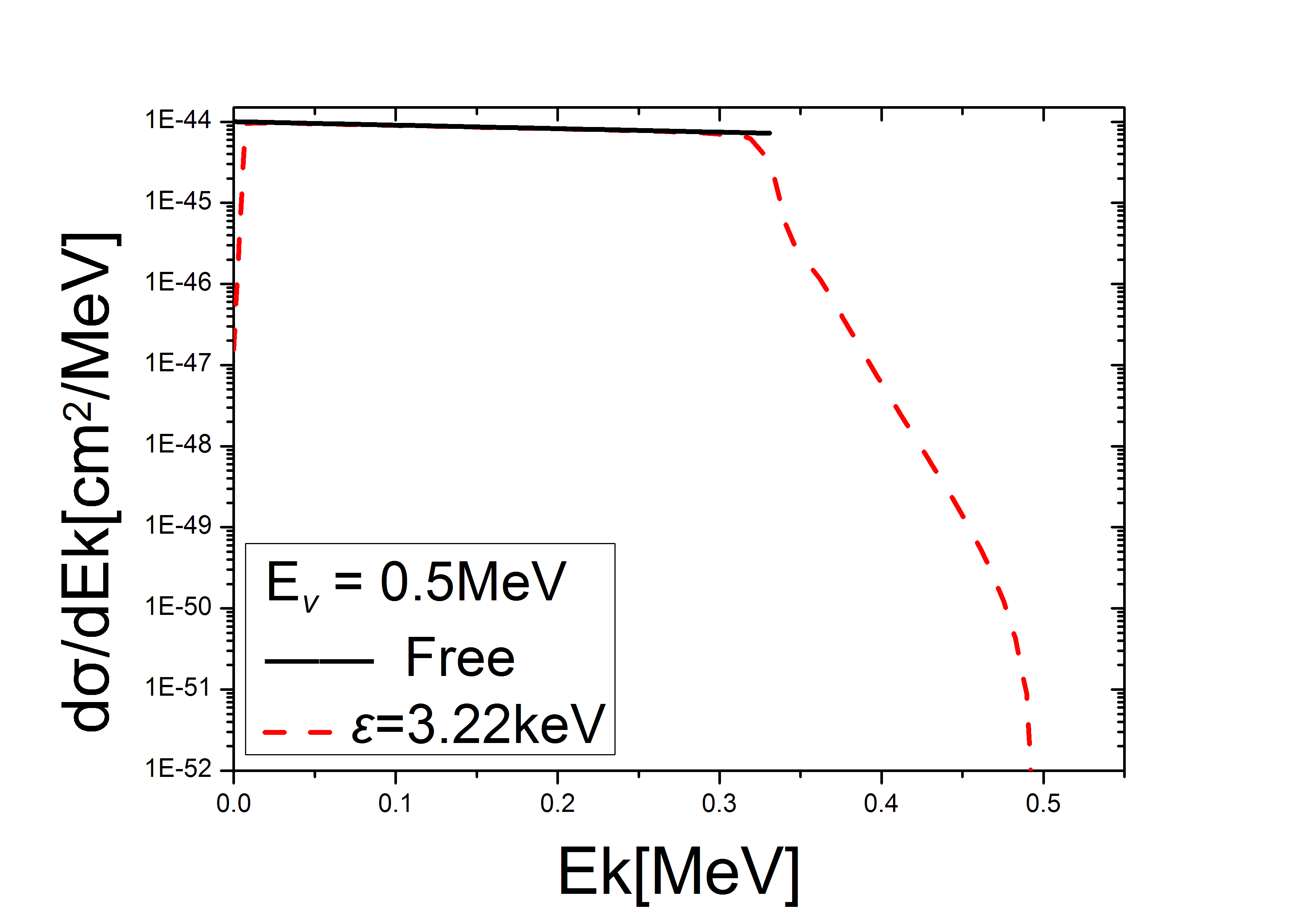
Figure 2: Differential cross section of the scattering of an electron neutrino with bound electron in $2s$ state of Ru atom. The black solid line is for the scattering with electron at rest with $E_{k}$ in the kinematically allowed range $[0,E_{\nu}/(1+m_{e}/(2E_{\nu}))]$. The binding energy is chosen as $\varepsilon=3.22$ keV.

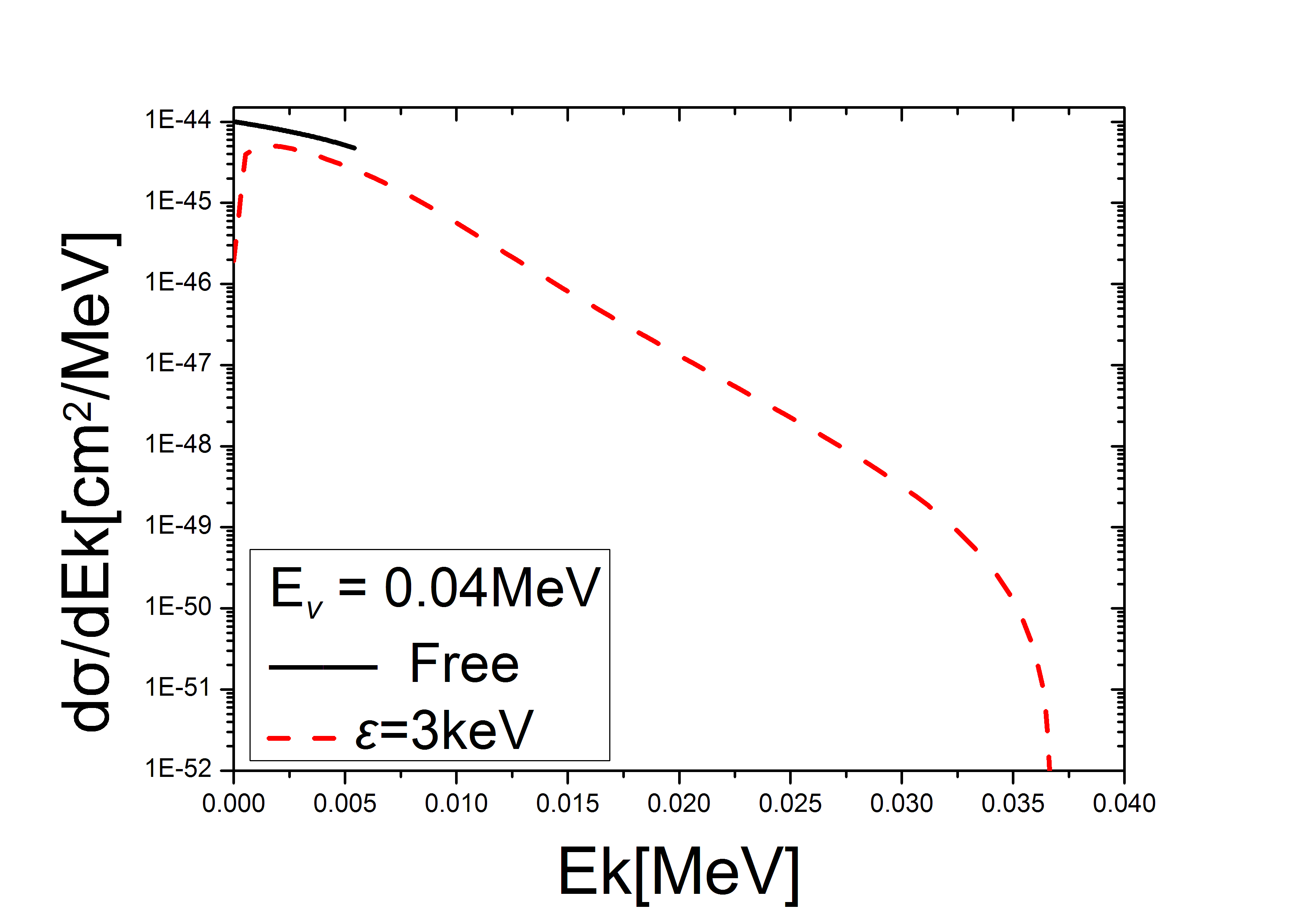
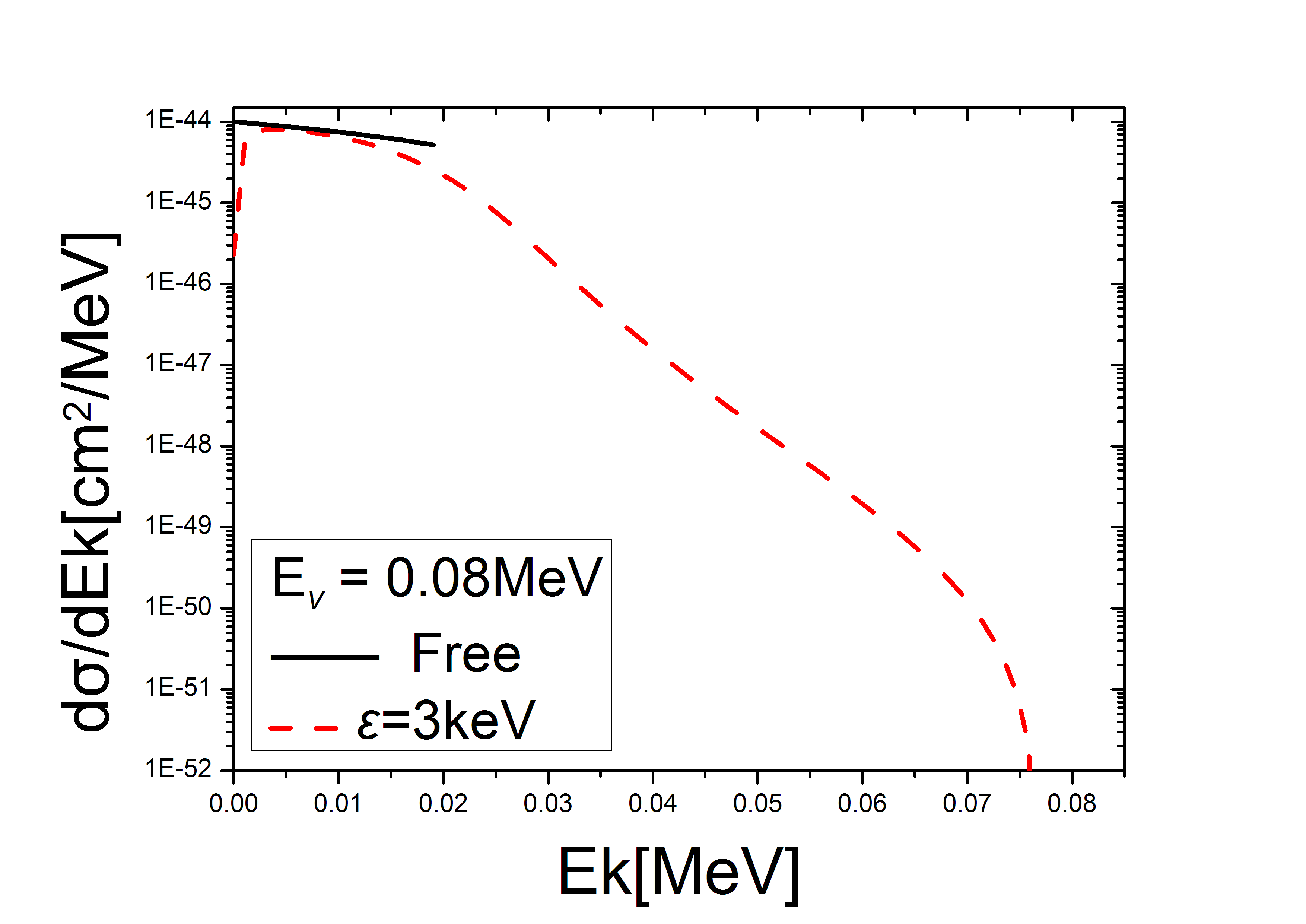
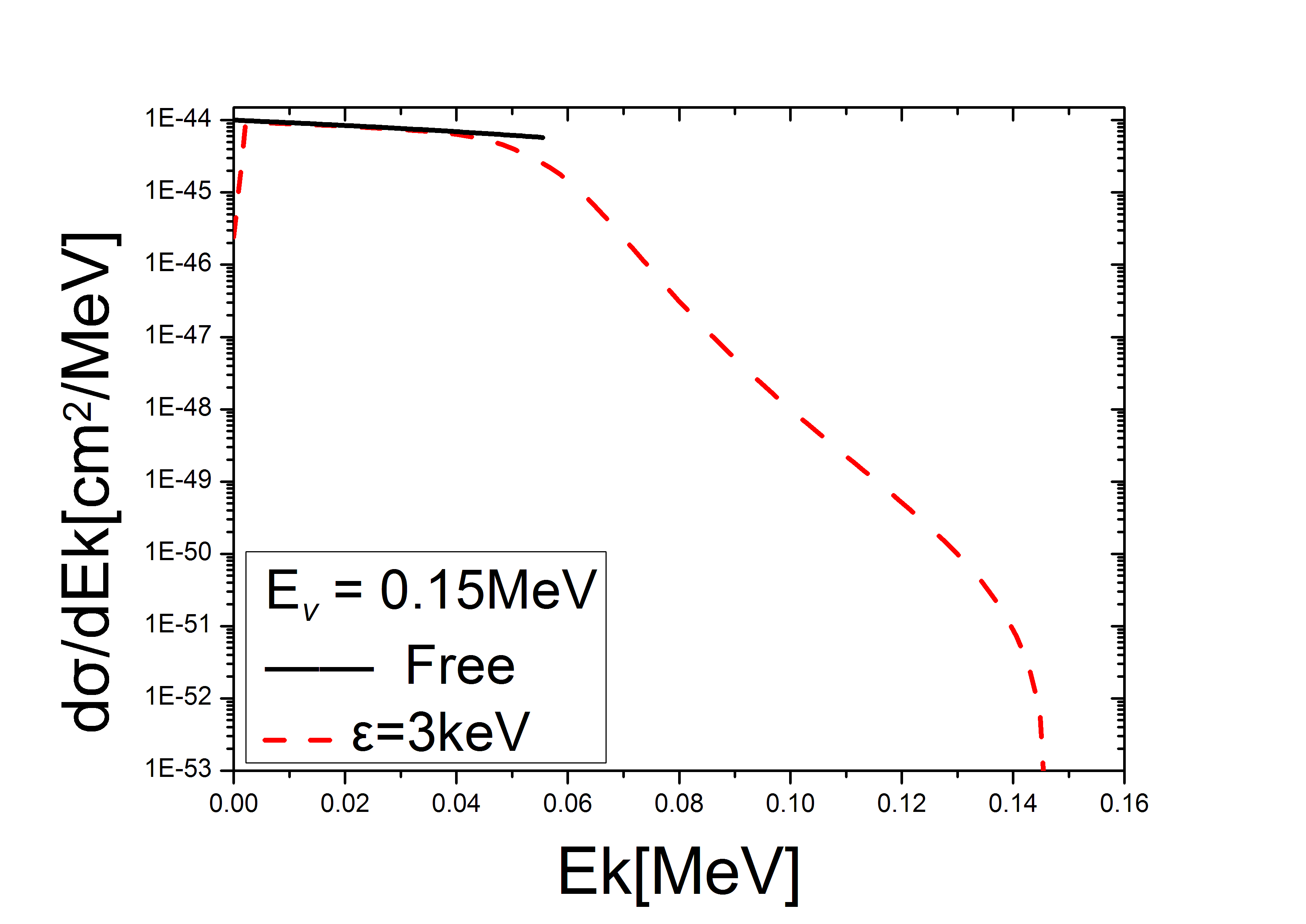
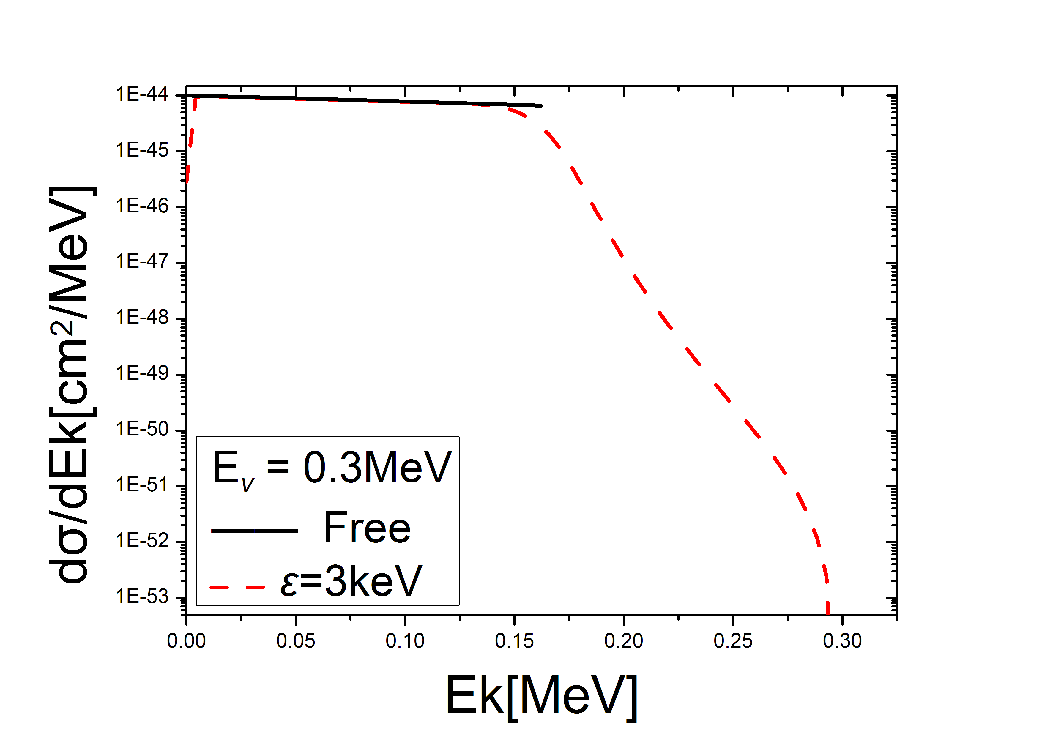
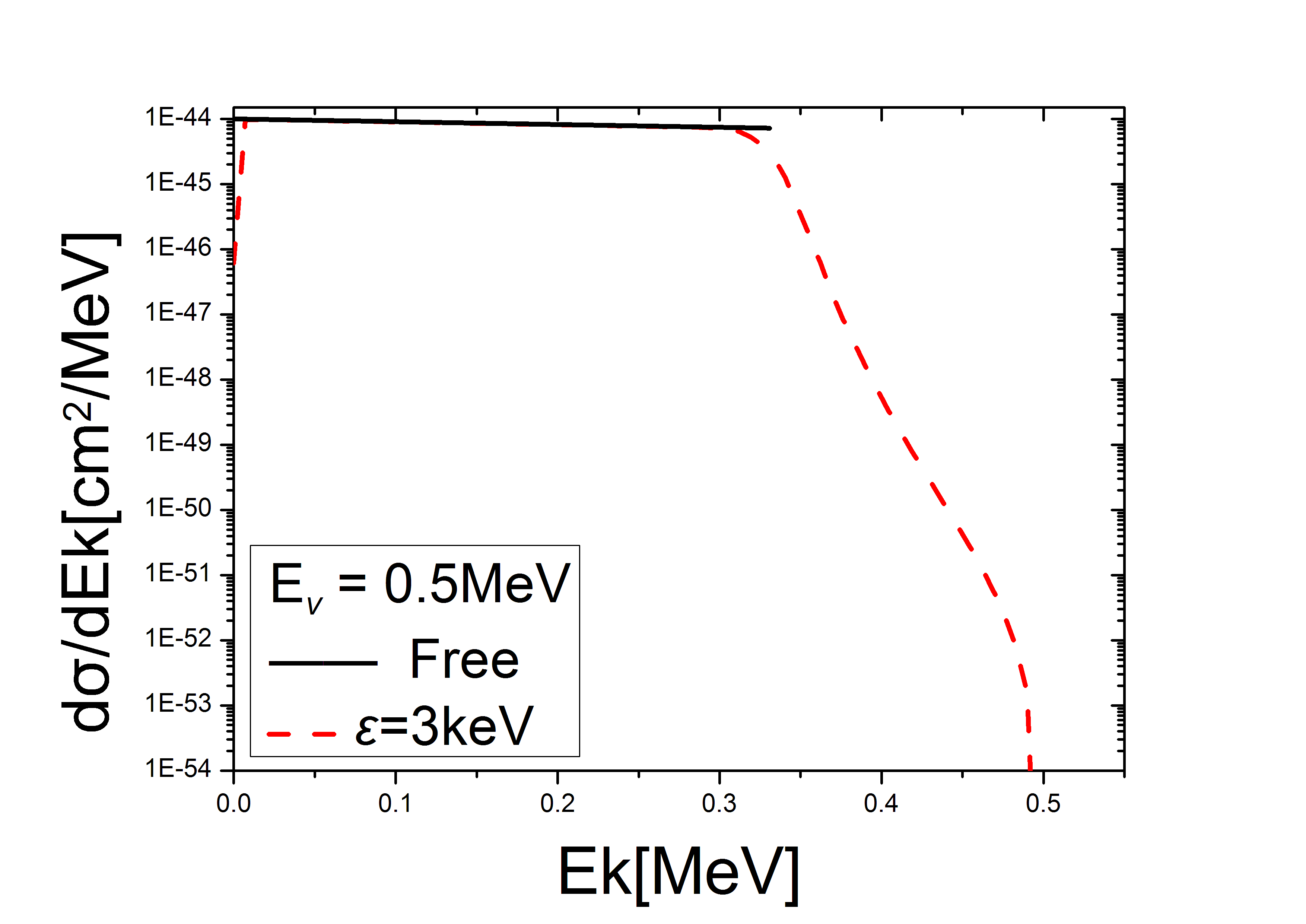
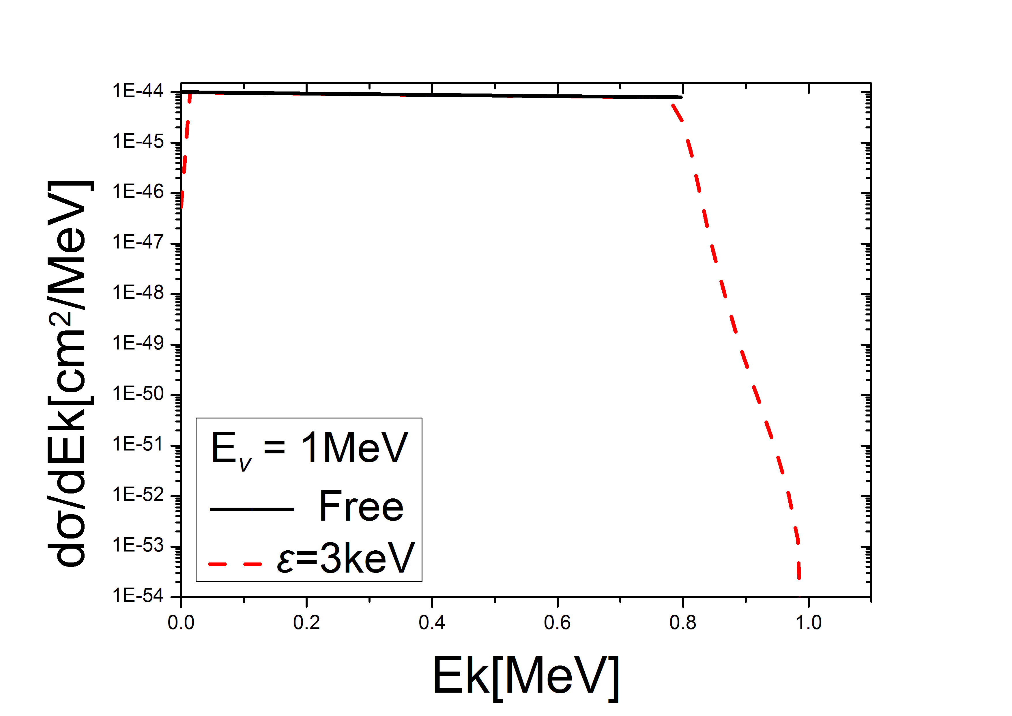
Figure 3: Differential cross section of the scattering of an electron neutrino with bound electron in $2p$ state of Ru atom.The black solid line is for the scattering with electron at rest with $E_{k}$ lies in the kinematically allowed range $[0,E_{\nu}/(1+m_{e}/(2E_{\nu}))]$. The binding energy is chosen as $\varepsilon=3$ keV.

In Fig. 1 we show the differential cross section for the scattering of an electron neutrino with electron in K shell of Ru atom. One can see that at $E_{k}\approx 0$ tail the differential cross section drops down sharply. As a comparison, one can see that the cross section of the scattering with free electron at rest remains constant for $E_{k}=0$. As noted in comment C) shown above, this is because the initial electron has a distribution of momentum and the probability of finding electron in the required momentum range, i.e. the range for reaching $E_{k}\approx 0$, is small.

In Fig. 1 we can see that the scattering of a neutrino with a bound electron has an $E_{k}$ spectrum wider than that of the scattering with free electron at rest. As shown in Eq. (10), the kinetic energy of the final electron in the scattering with free electron at rest lies in a limited range with a maximum value which can be much smaller than $E_{\nu}$ when $E_{\nu}<m_{e}$. In contrast, the final electron is allowed to get a kinetic energy as large as $E_{\nu}-\varepsilon$ for the scattering with bound electron, as noted in comment D) above. One can find that for $E_{\nu}\lower 3.01385pt\hbox{$\;\stackrel{{\scriptstyle\textstyle<}}{{\sim}}\;$}0.15$ MeV the difference between the allowed energy ranges of the scattering with free electron and the scattering with bound electron is very large. For $E_{\nu}>m_{e}$, the difference becomes negligible.

One can see in Fig. 1 that for large $E_{\nu}$ the cross section of the scattering with bound electron becomes close to that of the scattering with free electron at rest. In particular, for $E_{\nu}\lower 3.01385pt\hbox{$\;\stackrel{{\scriptstyle\textstyle>}}{{\sim}}\;$}0.3$ MeV the cross section of the scattering with bound electron agrees well with that of the free electron case in the kinematically allowed region of $E_{k}$ in the free electron case. Although there is still a tail beyond the range allowed by the scattering with free electron at rest, the differential cross section in tail region is suppressed by several orders of magnitude.

Figure 4: Differential cross section versus $E_{\nu}$, the energy of the initial neutrino, for the scattering of an electron neutrino with bound electron in Ru atom. The binding energies for 1s, 2s and 2p states are chosen the same as in Figs. 1, 2 and 3 saperately.The energy of the final electron is fixed as $E_{k}=42$ keV.

As a comparison we plot three lines in Fig. 1 for $\varepsilon=22.1$ keV and $\pm 20\%$ variation of this value of binding energy. One can see that $20\%$ variation does not lead to large difference for the scattering with $E_{\nu}>0.1$ MeV. It has impact to the scattering with $E_{\nu}=0.06$ MeV. In particular, there are visible differences close to the end of the tails in the plot for $E_{\nu}=0.06$ MeV. This corresponds to the change of the threshold for the production of a final electron with a particular energy. It’s not a surprise that this threshold would depend on value of $\varepsilon$.

In Fig. 2 we plot the differential cross section of the scattering of an electron neutrino with electron in $2s$ state. We can find phenomena similar to that discussed above for the scattering with electron in $1s$ state. A major difference is that the lines for the scattering with electron in $2s$ state get close to that of the free electron case at smaller $E_{\nu}$ compared to the lines of the scattering with electron in $1s$ state. One can see in Fig. 2 that for $E_{\nu}\lower 3.01385pt\hbox{$\;\stackrel{{\scriptstyle\textstyle>}}{{\sim}}\;$}0.06$ MeV the differential cross section of the scattering with bound electron is already quite close to that of the scattering with free electron in the energy range, $[0,E_{\nu}/(1+m_{e}/(2E_{\nu}))]$, allowed by the scattering with free electron.

In Fig. 3 we plot the differential cross section of the scattering of an electron neutrino with electron in $2p$ state of Ru atom. The plot is given for the cross section evaluated for the average momentum distribution $|\varphi_{2p}|^{2}$ of electrons in $2p$ state:

$$\frac{d\sigma_{2p}}{dE_{k}}=\int~{}d^{3}p_{B}~{}|\varphi_{2p}({\vec{p}}_{B})|^{2}\frac{d\sigma_{{\vec{p}}_{B}}}{dE_{k}},$$ (28)

where

$$|\varphi_{2p}({\vec{p}}_{B})|^{2}=\frac{1}{3}(|\varphi_{2p0}({\vec{p}}_{B})|^{2}+|\varphi_{2p+1}({\vec{p}}_{B})|^{2}+|\varphi_{2p-1}({\vec{p}}_{B})|^{2}).$$ (29)

For convenience we choose a universal binding energy $\varepsilon_{L}=3$ keV for $\varphi_{2p0}$ and $\varphi_{2p\pm 1}$. We note that $2p_{1\over 2}$ and $2p_{3\over 2}$ states correspond to linear combinations of $\varphi_{2p0}$ and $\varphi_{2p\pm 1}$ together with spinors. An advantage of computing Eq. (28) is that it’s invariant after recombination of wavefunctions $\varphi_{2p0}$ and $\varphi_{2p\pm 1}$. In particular, computation using $2p_{1\over 2}$ and $2p_{3\over 2}$ wavefunctions lead to the same result as in Eq. (29) after averaging contributions of all electrons in $2p_{1\over 2}$ and $2p_{3\over 2}$ states.

In Fig. 3 we can find phenomena similar to that discussed for the scattering with electron in $2s$ state. Similarly, we can find in Fig. 3 that for $E_{\nu}\lower 3.01385pt\hbox{$\;\stackrel{{\scriptstyle\textstyle>}}{{\sim}}\;$}0.06$ MeV the differential cross section of the scattering with bound electron is already quite close to that of the scattering with free electron in the energy range, $[0,E_{\nu}/(1+m_{e}/(2E_{\nu}))]$, allowed by the scattering with free electron at rest.

Figure 5: Differential cross section versus $E_{\nu}$, the energy of the initial neutrino, for the scattering of a muon neutrino with bound electron in Ru atom. The binding energies for 1s, 2s and 2p states are chosen the same as in Figs. 1, 2 and 3 saperately. The energy of the final electron is fixed as $E_{k}=42$ keV.

We have seen in Figs. 1,2,3 that the final electron has an energy range wider than that for the scattering with free electron at rest. In particular, one can show that neutrinos with energy $E_{\nu}<\frac{1}{2}(E_{k}+\sqrt{E_{k}^{2}+2E_{k}m_{e}})$ do not contribute to the differential cross section, Eq. (9), for a fixed $E_{k}>0$. If considering electron events of a particular kinetic energy $E_{k}$, some low energy neutrinos in the initial spectrum would be found not to contribute to this type of events when using the cross section of the scattering with free electron at rest. According to the above discussion, these low energy neutrinos can indeed contribute to this type of events when using the cross section of the scattering with bound electron.

In Fig. 4 we plot the differential cross section for $E_{k}=42$ keV versus the initial $E_{\nu}$. One can see in Fig. 4 that for the scattering of electron neutrino with free electron the cross section starts to be non-zero from a non-zero value of $E_{\nu}$ which is $(E_{k}+\sqrt{E_{k}^{2}+2m_{e}E_{k}})/2$ as discussed above. For the scattering with bound electron, the cross section starts to be non-zero from a much smaller value of $E_{\nu}$ than that of the scattering with free electron at rest. For $E_{\nu}$ close to the threshold value, the differential cross section of the scattering with bound electrons can start from a value infinitely close to zero. One can see that the lines for the scattering with electrons in 2s or 2p states are very close to the line for the scattering with free electron at rest in the kinematically allowed energy range of the scattering with free electron. Outside this allowed energy range, the cross sections of the scattering with electrons in 2s or 2p states decrease sharply for orders of magnitude. This means that the bound state features of 2s and 2p states just give small corrections to the scattering process. For comparison one can see that the line for the scattering with electron in 1s state is not very close to the line for the free electron case. There are visible differences between the line for the free electron case and the line for electron in 1s state up to $E_{\nu}\sim 0.2-0.3$ MeV. In Fig. 5 we give a plot similar to Fig.4 but for the scattering of muon neutrino with bound electrons. One can see phenomena similar to that in Fig. 4.

In Figs. 4 and 5 we have seen that the cross section of the scattering with bound electrons in L shell(2s or 2p states) agrees well with the cross section of the scattering with free electron at rest and the bound state features give small corrections to the scattering process. It’s natural to expect that the bound state features of electrons in M, N and O shells should give even smaller corrections compared that of the electrons in L shell. This is easy to understand because the binding energies of states in these shells are much smaller than that of the states in L shell, as can be seen in Table 1. According to this discussion we can approximate the cross section of the scattering with electrons in M, N and O shells as that of the scattering with free electron at rest.

Scattering of solar neutrino with bound electron in Ru atom

Sources	Fluxes ($10^{10}$ cm-2 s-1)	Energy(MeV)
pp	$6.0$ ($\pm 2\%$)	[0, 0.423]
pep	$0.014$($\pm 5\%$)	1.44
hep	$8.\times 10^{-7}$	[0, 18.78]
7Be	$0.47$($\pm 15\%$)	0.861
8B	$5.8\times 10^{-4}$ ($\pm 37\%$)	[0, 16.40]
13N	$0.06$ ($\pm 50\%$)	[0, 1.199]
15O	$0.05$ ($\pm 58\%$)	[0, 1.732]
17F	$5.2\times 10^{-4}$($\pm 46\%$)	[0, 1.74]

Table 2: Calculated solar neutrino fluxbahcall . Uncertainties of solar neutrino fluxes are shown in brackets.

Solar neutrinos are electron neutrinos produced in fusion reactions or in decays of radioactive nuclei. As can be seen in Table 2, solar neutrino fluxes are dominated by the pp neutrino and ⁷Be neutrino. Fluxes of ¹³N neutrinos, ¹⁵O neutrinos and pep neutrinos are also not small. Solar neutrinos also have a quite wide spectrum. For $E_{\nu}\lower 3.01385pt\hbox{$\;\stackrel{{\scriptstyle\textstyle<}}{{\sim}}\;$}0.4$ MeV, the solar neutrino spectrum is dominated by the pp neutrinos. For $E_{\nu}\lower 3.01385pt\hbox{$\;\stackrel{{\scriptstyle\textstyle>}}{{\sim}}\;$}1.74$ MeV, it is dominated by ⁸B neutrinos. In between $0.4$ MeV and $1.74$ MeV, major contributions are from ⁷Be neutrinos, ¹³N neutrinos and ¹⁵O neutrinos  bahcall .

Solar electron neutrinos oscillate into muon neutrinos and tau neutrinos in propagation from the Sun to the Earth w ; ms . The probability of electron neutrinos surviving as electron neutrinos after propagation to the Earth depends on the energy of the neutrinos and on the matter density profile in the Sun. In  Liao0 it was shown that the survival probability of solar electron neutrinos can be well described using a formula with an average density associated with the neutrino production in the Sun. Since eight types of solar neutrinos, as shown in Table 2, have different production distribution in the Sun, the average survival probabilities are different for different types of solar neutrinos. For solar neutrino of type k, we label $P_{k}$ as the survival probability of the electron neutrinos after propagation to the Earth. $P_{k}$ can be found in  Liao0 . The survival probability also depends on the mass squared difference, $\Delta m^{2}_{21}$, and the vacuum mixing angle $\theta_{12}$. When computing $P_{k}$ we use

$$\Delta m^{2}_{21}=7.62\times 10^{-5}~{}\textrm{eV}{{}^{2}},~{}~{}sin^{2}\theta_{12}=0.32.$$ (30)

In the previous section we find that in the scattering with bound electrons solar neutrinos in a very wide energy range can contribute to the events with final electron of a kinetic energy $E_{k}\approx 42$ keV. In particular, this means that neutrinos with energy less than $\frac{1}{2}(E_{k}+\sqrt{E_{k}^{2}+2E_{k}m_{e}})$, that is $\lower 3.01385pt\hbox{$\;\stackrel{{\scriptstyle\textstyle<}}{{\sim}}\;$}126$ keV for $E_{k}\approx 42$ keV, can contribute to the events with $E_{k}\approx 42$ keV.

Using the calculated neutrino fluxes and the energy spectrum for all eight types of neutrinos given in  bahcall , we can compute the rate of events in the interested energy range, i.e. in range $E_{k}\approx 42$ keV. The differential event rate of contributions of neutrinos with energy $E_{\nu}$ is computed as follows

$$\frac{dR}{dE_{\nu}}=\frac{d\sigma_{\nu_{e}}(E_{\nu})}{dE_{k}}~{}N_{e}~{}\sum_{k}F^{k}_{\nu}(E_{\nu})P_{k}+\frac{d\sigma_{\nu_{\mu}}(E_{\nu})}{dE_{k}}~{}N_{e}~{}\sum_{k}F^{k}_{\nu}(E_{\nu})(1-P_{k}),$$ (31)

where $k$ runs over eight types of solar neutrinos, $F^{k}_{\nu}$ the flux distribution of type k solar neutrino, $N_{e}$ the number of electrons in Ru target. $\sigma_{\nu_{e}}$ and $\sigma_{\nu_{\mu}}$ are the cross sections for scattering of electron neutrino and muon neutrino separately. $P_{k}=P_{k}(E_{\nu})$ is the survival probability of electron neutrino described above. $1-P_{k}$ is the probability of solar electron neutrinos oscillating into muon neutrinos and tau neutrinos. Since the scattering of $\nu_{\mu}$ and $\nu_{\tau}$ with electrons are universal, we use $\sigma_{\mu}$ in Eq. (31). For simplicity, we neglect the Earth matter effect in our calculation since it would lead to at most about $4\%$ corrections for large energy solar neutrino Liao0 . For solar neutrinos with energy less about 1 MeV, the Earth matter effect would be smaller than $1\%$ and can be safely neglected.

The differential cross section used in (31) is an average for the scattering with all electrons in the neutral Ru atom. It is written as

$$\frac{d\sigma_{\nu_{e}}}{dE_{k}}=\frac{1}{Z}\sum_{l}~{}n_{l}~{}\frac{d\sigma_{l}}{dE_{k}},$$ (32)

where $l$ runs over all states in Table 1, $n_{l}$ the number of electrons in state $l$, $Z=44$ for Ru atom. For electrons in M, N and O shells we approximate $d\sigma_{l}/dE_{k}$ as the same as that of the scattering with free electron at rest, as discussed in the last section. Similarly we have an expression for $d\sigma_{\nu_{\mu}}$.

The total rate is obtained after integrating Eq. (31) over $E_{\nu}$. For 10 tons of ¹⁰⁶Ru we obtain

$$R=0.21\times\frac{\Delta E_{k}}{10~{}\textrm{eV}}~{}\textrm{year}^{-1}.$$ (33)

We can see in Eq. (33) that if the energy of final electron can be measured to a resolution of $10$ eV, solar neutrinos would produce about 0.2 electron events in the scattering with electrons in 10 tons of ¹⁰⁶Ru target. In Liao it was shown that for $\theta$, the mixing of the sterile neutrino DM to electron neutrino, of order $\theta^{2}=10^{-6}$, the $\nu_{s}$ capture by ¹⁰⁶Ru can produce tens of events per year. Eq. (33) says that background from the scattering with solar neutrinos allows us to measure $\theta^{2}$ to a precision of $10^{-7}$ if the energy of the final electron can be measured to a precision of 10 eV. If the energy of final electron can only be measured to a resolution of 100 eV, this background allows us to measure $\theta^{2}$ to a precision of $10^{-6}$.

In calculation of the events rate we find that the scattering with solar neutrinos of energy $\lower 3.01385pt\hbox{$\;\stackrel{{\scriptstyle\textstyle<}}{{\sim}}\;$}126$ keV gives small contribution to the result given in Eq. (33). This is because 1) the cross section in this energy range is suppressed compared to that in the energy range $E_{\nu}\lower 3.01385pt\hbox{$\;\stackrel{{\scriptstyle\textstyle>}}{{\sim}}\;$}126$ keV, as can be seen in Figs. 4 and 5; 2) the solar neutrinos in this energy range only account for about $7\%$ of the total solar neutrino flux. We note that electron after passing out of the target can lose energy and create broadening of spectrum. But this does not change our result in Eq. (33) because the event rate R varies very slowly with $E_{k}$. A spectrum broadening of $10-100$ eV level just gives rise to a mild re-distribution of events in the original spectrum and it would not change the estimate of a continuous spectrum in a range as wide as a few to around ten keV.

Conclusion:

In summary we have studied in detail the scattering of solar neutrinos with bound electrons in Ru atom. This study is helpful to clarify the background events caused by solar neutrinos in the search of keV scale sterile neutrino DM using ¹⁰⁶Ru target.

We concentrate on the scattering of solar neutrinos with electrons in the 1s, 2s and 2p states in Ru atom. We find that for small $E_{\nu}$ the scattering of neutrinos with free electron at rest and the scattering with bound electron can be quite different. For large $E_{\nu}$, the difference tends to be small. For $E_{\nu}>m_{e}$, the difference tends to be negligible. For events of final electrons with a fixed kinetic energy, say $E_{k}\approx 42$ keV, we find that the scattering of neutrino with free electron at rest starts to contribute when $E_{\nu}\lower 3.01385pt\hbox{$\;\stackrel{{\scriptstyle\textstyle>}}{{\sim}}\;$}126$ keV. On the other hand, the scattering of neutrino with bound electron starts to contribute from values of $E_{\nu}$ much smaller than $126$ keV. This means that low energy part of the solar neutrino spectrum can contribute to the scattering. This part of solar neutrino spectrum would be neglected when using the cross section of the scattering of neutrino with free electrons at rest. Fortunately, solar neutrinos with energy $E_{\nu}\lower 3.01385pt\hbox{$\;\stackrel{{\scriptstyle\textstyle<}}{{\sim}}\;$}126$ keV only account for about $7\%$ of the total neutrino flux and the scattering with bound electrons does not give a large difference compared to that computed using the scattering with free electron at rest.

We estimate the event rate of electrons produced by the scattering of solar neutrinos with electrons in Ru atom. We find that events of final electrons having $E_{k}\approx 42$ keV are $0.2$ per year if the energy of the final electron can be measured to a precision of $10$ eV. This allows to search for the $\nu_{s}$ DM with a mixing of $\nu_{s}$ and $\nu_{e}$ at order $\theta^{2}=10^{-7}$. If the energy of the final electron can be measured to a precision of $100$ eV, it allows to search for the $\nu_{s}$ DM with a mixing of $\nu_{s}$ and $\nu_{e}$ at order $\theta^{2}=10^{-6}$. For 10 kg ³T as used in Liao for the search of $\nu_{s}$ DM, the rate of this type of background events is smaller by about three orders of magnitude. It does not create problem for the search of $\nu_{s}$ DM using ³T target. We find that for larger energy resolution, the event rate of the background is larger. To avoid the pollution of this type of electron events in the search of sterile neutrino DM, we should have good energy resolution to suppress this type of background events.

- (1) J. Sommer-Larsen, A. Dolgov, Astrophys. J. 551, 608(2001); P. Colin, V. Avila-Reese, O. Valenzuela, Astrophys. J. 542, 622(2000).
- (2) C. Destri, H. J. de Vega and N. G. Sanchez, New Astron. 22, 39(2013); Astrop. Phys. 46, 14 (2013).
- (3) W. Liao, Phys. Rev. D82, 073001(2010).
- (4) W. Liao, in Highlights and Conclusions of the Chalonge CIAS Meudon Workshop 2012, eds. P.L. Biermann, H. J. de Vega, N.G. Sanchez, arXiv: 1305.7452.
- (5) T. Asaka, S. Blanchet and M. Shaposhnikov, Phys. Lett. B631, 151(2005).
- (6) For recent reviews, see A. Merle, Int. J. Mod. Phys. D22, 1330020(2013); M. Drewes, Int. J. Mod. Phys. E22, 1330019(2013).
- (7) S. Dodelson and L. W. Windrow, Phys. Rev. Lett. 72, 17(1994).
- (8) A. D. Dolgov and S. H. Hansen, Astropart. Phys. 16, 339 (2002); K. Abazajian, G.M. Fuller, and M. Patel, Phys. Rev. D64, 023501 (2001); K. Abazajian, G.M. Fuller, and W.H. Tucker, Astrophys. J. 562, 593 (2001).
- (9) A. Boyarsky, et.al., Phys. Rev. Lett. 102, 201304(2009).
- (10) M. Shaposhnikov and I. Tkachev, Phys. Lett. B639, 414 (2006).
- (11) K. Petraki and A. Kusenko, Phys. Rev. D77, 065014 (2008).
- (12) F. Bezrukov, H. Hettmansperger, M. Lindner, Phys. Rev. D81, 085032(2010).
- (13) A. Boyarsky, et.al., Phys. Rev. Lett. 97, 261302(2006).
- (14) A. Boyarsky, J. Nevalainen and O. Ruchayskiy, Astron. Astrophys. 471, 51(2007).
- (15) A. Boyarsky, D. Iakubovskyi, O. Ruchayskiy and V. Savchenko, MNRAS 387, 1361(2008).
- (16) A. Boyarsky, J. Lesgourgues, O. Ruchayskiy, M. Viel, JCAP 0905, 012(2009).
- (17) A. Boyarsky, O. Ruchayskiy, D. Iakubovskyi, JCAP 0903, 005(2009).
- (18) M. Shaposhnikov, Nucl. Phys. B763, 49(2007).
- (19) M. Lindner, A. Merle, V. Niro, JCAP 1101 (2011) 034.
- (20) C.-Q. Geng, R. Takahashi, Phys. Lett. B710, 324(2012).
- (21) L. Canetti, M. Drewes, M. Shaposhnikov, Phys. Rev. Lett. 110, 061801(2013).
- (22) D. J Robinson, Y. Tsai, JHEP 1208 (2012) 161.
- (23) A. Boyarsky, D. Iakubovskyi, O. Ruchayskiy, Phys. Dark Univ. 1, 136(2012).
- (24) Y. F. Li and Z. Z. Xing, JCAP 1108(2011)006.
- (25) Y. F. Li and Z. Z. Xing, Phys. Lett. B695, 205(2011).
- (26) H. de Vega, et.al, Nucl. Phys. B866, 177 (2013).
- (27) F. Bezrukov and M. Shaposhnikov, Phys. Rev. D75, 053005(2007).
- (28) S. Ando and A. Kusenko, Phys. Rev. D81, 113006(2010).
- (29) David R. Lide, ed., CRC Handbook of Chemistry and Physics, CRC Press, Boca Raton, FL, 2005
- (30) J. A. Bearden and A. F. Burr, Rev. Mod. Phys. 39, 125(1967).
- (31) Review of Particle Physics, Phys. Rev. D86, 010001(2012).
- (32) M. A. Coplan et al., Rev. Mod. Phys. 66, 985(1994).
- (33) Neutrino Astrophysics, J. N. Bahcall, Cambridge University Press 1989; see also online data at website: http://www.sns.ias.edu/ jnb/SNdata/sndata.html
- (34) L. Wolfenstein, Phys. Rev. D 17, 2369 (1978); L. Wolfenstein, in ”Neutrino-78”, Purdue Univ. C3 - C6, (1978).
- (35) S. P. Mikheyev and A. Yu. Smirnov, Yad. Fiz. 42, 1441 (1985) [ Sov. J. Nucl. Phys. 42, 913 (1985)]; Nuovo Cim. C9, 17 (1986); S. P. Mikheyev and A. Yu. Smirnov, ZHETF, 91, (1986), [Sov. Phys. JETP, 64, 4 (1986)] (reprinted in ”Solar neutrinos: the first thirty years”, Eds. J.N.Bahcall et. al.).
- (36) P. C. de Holanda, W. Liao, A. Yu. Smirnov, Nucl. Phys. B 702, 307(2004).