Wigner localization in quantum dots from Kohn-Sham density functional theory without symmetry breaking

Abstract

We address low-density two-dimensional circular quantum dots with spin-restricted Kohn-Sham density functional theory. By using an exchange-correlation functional that encodes the effects of the strongly-correlated regime (and that becomes exact in the limit of infinite correlation), we are able to reproduce characteristic phenomena such as the formation of ring structures in the electronic total density, preserving the fundamental circular symmetry of the system. The observation of this and other well-known effects in Wigner-localized quantum dots such as the flattening of the addition energy spectra, has until now only been within the scope of other, numerically more demanding theoretical approaches.

I Introduction

The effects of strong electronic correlation in low-dimensional semiconductor nanostructures have attracted large research interest for decades, both from purely fundamental and from applied points of view.Ghosal et al. (2006); Guclu et al. (2008); Yannouleas and Landman (2007); Auslaender et al. (2005); Kristinsdottir et al. (2011) The high degree of tunability of, e.g., quantum wires or quantum dots, nowadays easily realized in laboratories,Auslaender et al. (2005); Kristinsdottir et al. (2011) renders them a fertile playground to investigate strong-correlation phenomena. For example, it is well known that, for sufficiently low densities, such finite systems may display charge localization,Creffield et al. (1999); Egger et al. (1999); Yannouleas and Landman (1999); Reimann et al. (2000); Filinov et al. (2001); Pederiva et al. (2002); Ghosal et al. (2007) reminiscent of the Wigner crystallization of the bulk electron gasWigner (1934) and a consequence of the dominance of the Coulomb repulsion over the electronic kinetic energy. From the practical side, potential applications of Wigner-localized systems include the design and manipulation of qubits and quantum computing devices,Weiss et al. (2006); Deshpande and Bockrath (2008); Taylor and Calarco (2008); Yannouleas and Landman (2007) or the realization of infrared sensors to control the electron filling in semiconductor nanostructures.Ballester et al. (2010)

Along with the fundamental and practical interest, strongly-correlated systems are well-known to pose serious challenges for the different theoretical approaches commonly used to study them. On the one hand, the configuration interaction (CI) method becomes numerically unaffordable if one wants to treat more than five or six electrons.Reimann and Manninen (2002); Rontani et al. (2006); Ghosal et al. (2007) By using coupled-cluster methods, which allow for a larger basis set, it has very recently been shown that the number of particles can be raised up to twelve in two-dimensional quantum dots.Waltersson et al. (2013) Other wavefunction approaches, such as quantum Monte Carlo (QMC) methodsGhosal et al. (2006, 2007); Guclu et al. (2008) or density matrix renormalization group (DMRG),Stoudenmire et al. (2012) can treat larger systems (still less than $\sim 10^{2}$ particles) but face limitations as well if the correlations become too strong.Ghosal et al. (2007) On the other hand, spin-unrestricted Hartree-Fock (HF)Yannouleas and Landman (1999, 2007) or density-functional Borgh et al. (2005) approaches, much less computationally demanding, mimic the effects of strong correlation by breaking the spin and other symmetries of the system. This makes them much less reliable than wavefunction methods, sometimes with unphysical results and controversial interpretations.Anisimov et al. (1991); Harju et al. (2004); Borgh et al. (2005); Stoudenmire et al. (2012)

Kohn-Sham (KS) density functional theory (DFT), in its original restricted formulation,Hohenberg and Kohn (1964); Kohn and Sham (1965) has been known for a long time to deliver very poor results when applied to strongly-correlated systems. The reason for this is not fundamental, as KS DFT is, in principle, an exact theory. The problem is that the available approximations for the exchange-correlation functional fail in the strongly-correlated regime, Anisimov et al. (1991); Cohen et al. (2008); Ghosal et al. (2007); Abedinpour et al. (2007) sometimes making it extremely difficult to even get converged results at all.Zeng et al. (2009) For example, the local-density approximation (LDA) wrongly predicts largely delocalized electronic densities in strongly-correlated quantum wires,Abedinpour et al. (2007) being unable to reproduce the expected $N$-electron-peak structure due to charge localization.Abedinpour et al. (2007)

Recently, a novel way of constructing exchange-correlation functionals for KS DFT has been proposed,Malet and Gori-Giorgi (2012); Malet et al. (2013) based on the exact strong-coupling limit of DFT, which was formulated a few years ago within the so-called strictly-correlated-electrons (SCE) formalism.Seidl et al. (2007); Gori-Giorgi et al. (2009a); Gori-Giorgi and Seidl (2010) The first applications on quasi-one-dimensional quantum wiresMalet and Gori-Giorgi (2012); Malet et al. (2013) have shown that the resulting exchange-correlation functional is able to qualitatively describe arbitrary correlation regimes without artificially breaking any symmetry. This is achieved since the SCE functional is able to create barriers (or “bumps”) in the corresponding Kohn-Sham potential, which are a known feature of the exact one.Buijse et al. (1989); Helbig et al. (2009) Precisely these barriers can localize the charge density, avoiding the need of symmetry breaking to describe systems in which charge localization effects are important.

In this paper, we extend this approach to the study of two-dimensional circularly-symmetric quantum dots with parabolic confinement. By considering different confinement strengths, we investigate the crossover between the weakly-interacting and the strongly-correlated regimes. In particular, we reproduce well-known features of low-density quantum dots such as the formation of sharp rings in the electronic densityGhosal et al. (2006, 2007) or the flattening of the addition energy spectra.Yannouleas and Landman (1999) Due to the relatively low computational cost of our approach, we thus provide here an alternative powerful tool to study these kinds of systems.

II Quantum Dot Model

We consider two-dimensional (2D) quantum dots with $N$ electrons, laterally confined by a parabolic potential and described by the Hamiltonian (see, e.g., Ref. Reimann and Manninen, 2002)

$$\hat{H}=\sum_{i=1}^{N}\left(-\frac{\hbar^{2}}{2{m^{*}}}\nabla_{i}^{2}+m^{*}\frac{\omega^{2}}{2}r_{i}^{2}\right)+\frac{e^{2}}{\epsilon}\sum_{i=1}^{N-1}\sum_{j=i+1}^{N}\frac{1}{|\mathbf{r}_{i}-\mathbf{r}_{j}|},$$ (1)

where $m^{*}$ is the effective mass and $\epsilon$ the dielectric constant. We use effective Hartree (H^∗) units ($\hbar=1$, $a_{B}^{*}=\frac{\epsilon}{m^{*}}a_{B}=1$, $e=1$, $m^{*}=1$) throughout the rest of the paper.

The correlation regime is determined by the confinement strength: small (large) values of $\omega$ correspond to low (high) densities, for which the Coulomb repulsion dominates over (is dominated by) the kinetic energy. In order to characterize the correlation quantitatively, one defines the so-called electron gas parameter. In 2D it is given in terms of the electronic density as $r_{s}=(\pi\bar{n})^{-1/2}$, where $\bar{n}\equiv\int\rho(\mathbf{r})^{2}d\mathbf{r}/N$ is the average electron density. In the first calculations presented here, we have considered $N=1,\dots,10$ and $\omega\in[0.001,1]$, corresponding to values of $r_{s}$ between $\sim 1$ and 68.

In the non-interacting case, the eigenfunctions of the system are the so-called Fock-Darwin states,Jacak et al. (1998) with associated energies given by

$$\varepsilon_{n,m}=2\omega\left(n+\frac{1}{2}+\frac{|m|}{2}\right)\;,$$ (2)

where $m\in{\mathbb{Z}}$ and $n\in{\mathbb{N}}_{0}$ are, respectively, the angular and radial quantum numbers.

III Theoretical Approach

III.1 KS DFT with the SCE functional

We use the zeroth-order “KS-SCE DFT” approach, which was introduced in Ref. Malet and Gori-Giorgi, 2012 and described in more detail in Ref. Malet et al., 2013. Essentially, the method consists of solving the standard spin-restricted Kohn-Sham equations,Kohn and Sham (1965)

$$\left(-\frac{\nabla^{2}}{2}+v_{\rm KS}[\rho](\mathbf{r})\right)\phi_{i}(\mathbf{r})=\varepsilon_{i}\phi_{i}(\mathbf{r})\;,$$ (3)

where $v_{\rm KS}[\rho](\mathbf{r})$ is the Kohn-Sham potential

$$v_{\rm KS}[\rho](\mathbf{r})=v_{\rm ext}[\rho](\mathbf{r})+v_{\rm Hartree}[\rho](\mathbf{r})+v_{\rm xc}[\rho](\mathbf{r})\;,$$ (4)

and $v_{\rm xc}[\rho](\mathbf{r})$ an approximate exchange-correlation potential that is constructed from the functional derivative of the exact strong-interaction limit of the Hohenberg-Kohn functional. The resulting potential is able to capture the features of the strongly-correlated regime without introducing any spin or spatial symmetry breaking in the system. Below we briefly describe how the functional and the potential are built, and we refer the reader to Ref. Malet et al., 2013 for further details.

The strictly-correlated-electrons (SCE) functional $V_{\rm ee}^{\rm SCE}[\rho]$ of Seidl and co-workersSeidl (1999); Seidl et al. (1999, 2000, 2007) is defined as the minimum possible electron-electron repulsion in a given smooth density $\rho(\mathbf{r})$:

$$V_{\rm ee}^{\rm SCE}[\rho]\equiv\min_{\Psi\to\rho}\langle\Psi|\hat{V}_{\rm ee}|\Psi\rangle,$$ (5)

where $\hat{V}_{\rm ee}$ is the Coulomb repulsion operator, i.e., the last term in Eq. (1). It can be shown that in the low-density (or strong-interaction) limit, the Hohenberg-Kohn functional tends asymptotically to $V_{\rm ee}^{\rm SCE}[\rho]$.Malet et al. (2013) The SCE functional is the natural counterpart of the KS kinetic energy $T_{s}[\rho]$: the latter defines a reference system of non-interacting electrons with the same density of the physical system, while the former introduces a reference system (again with the same density) in which the electrons are infinitely (or perfectly) correlated, in the sense that the position of one of them determines all the relative positions in order to minimize the total Coulomb repulsion.

Thus, in the SCE system, if one electron (which we can label as “1” and take as a reference) is at position $\mathbf{r}_{1}\equiv\mathbf{r}$, the positions of the remaining $N-1$ electrons are given by the so-called co-motion functions, $\mathbf{r}_{i}\equiv\mathbf{f}_{i}[\rho](\mathbf{r})$ ($i=2,\dots,N$), which are non-local functionals of the density. They satisfy the differential equationSeidl et al. (2007)

$$\rho(\mathbf{r})d\mathbf{r}=\rho(\mathbf{f}_{i}(\mathbf{r}))d\mathbf{f}_{i}(\mathbf{r})\;,$$ (6)

or, equivalently, are such that the probability of finding one electron at position $\mathbf{r}$ is the same of finding the electron $i$ at $\mathbf{f}_{i}(\mathbf{r})$. The co-motion functions also satisfy the following cyclic group properties, which are a consequence of the indistinguishability of the electrons, ensuring that there is no dependence on which electron is chosen as reference, Seidl et al. (2007)

$$\begin{split}&\mathbf{f}_{1}(\mathbf{r})\equiv\mathbf{r},\\ &\mathbf{f}_{2}(\mathbf{r})\equiv\mathbf{f}(\mathbf{r}),\\ &\mathbf{f}_{3}(\mathbf{r})=\mathbf{f}(\mathbf{f}(\mathbf{r})),\\ &\mathbf{f}_{4}(\mathbf{r})=\mathbf{f}(\mathbf{f}(\mathbf{f}(\mathbf{r}))),\\ &\qquad\ \vdots\\ &\underbrace{\mathbf{f}(\mathbf{f}(\ldots\mathbf{f}(\mathbf{f}(\mathbf{r}))))}_{\text{$N$ times}}=\mathbf{r}.\end{split}$$ (7)

Notice that the SCE system describes a smooth $N$-electron quantum-mechanical density by means of an infinite superposition of degenerate classical configurations, which fulfill Eq. (6) for every $\mathbf{r}$. The square modulus of the corresponding wave function (which becomes a distribution in this limitButtazzo et al. (2012); Cotar et al. (2013)) is given by

$$|\Psi_{\rm SCE}(\mathbf{r}_{1},\mathbf{r}_{2},\dots,\mathbf{r}_{N})|^{2}=\frac{1}{N!}\sum_{\wp}\int d\mathbf{r}\,\frac{\rho(\mathbf{r})}{N}\,\delta(\mathbf{r}_{1}-\mathbf{f}_{\wp(1)}(\mathbf{r}))\\ \times\delta(\mathbf{r}_{2}-\mathbf{f}_{\wp(2)}(\mathbf{r}))\cdots\delta(\mathbf{r}_{N}-\mathbf{f}_{\wp(N)}(\mathbf{r}))\;,$$ (8)

where $\wp$ denotes a permutation of ${1,\dots,N}$, such that $\rho(\mathbf{r})=N\int|\Psi_{\rm SCE}(\mathbf{r},\mathbf{r}_{2},\dots,\mathbf{r}_{N})|^{2}\,d\mathbf{r}_{2}\cdots d\mathbf{r}_{N}$. The SCE system can thus be visualized as a “floating” Wigner crystal in a metricGori-Giorgi et al. (2009b) that describes the smooth density distribution $\rho(\mathbf{r})$.

In terms of the co-motion functions, the SCE functional $V_{\rm ee}^{\rm SCE}[\rho]$ of Eq. (5) is given bySeidl et al. (2007); Mirtschink et al. (2012)

$$\begin{split}V_{\rm ee}^{\rm SCE}[\rho]&=\int d\mathbf{r}\,\frac{\rho(\mathbf{r})}{N}\sum_{i=1}^{N-1}\sum_{j=i+1}^{N}\frac{1}{|\mathbf{f}_{i}(\mathbf{r})-\mathbf{f}_{j}(\mathbf{r})|}\\ &=\frac{1}{2}\int d\mathbf{r}\,\rho(\mathbf{r})\sum_{i=2}^{N}\frac{1}{|\mathbf{r}-\mathbf{f}_{i}(\mathbf{r})|}\;.\end{split}$$ (9)

Another important property of the SCE system is the following: since the position of one electron at a given $\mathbf{r}$ determines the other $N-1$ electronic positions, the net Coulomb repulsion acting on an electron at a certain position $\mathbf{r}$ becomes a function of $\mathbf{r}$ itself. This force can be written in terms of the negative gradient of some one-body local potential $v_{\rm SCE}(\mathbf{r})$,Malet et al. (2013) such that

$$-\nabla v_{\rm SCE}[\rho](\mathbf{r})=\sum_{i=2}^{N}\frac{\mathbf{r}-\mathbf{f}_{i}[\rho](\mathbf{r})}{|\mathbf{r}-\mathbf{f}_{i}[\rho](\mathbf{r})|^{3}}\;.$$ (10)

In turn, $v_{\rm SCE}[\rho](\mathbf{r})$ satisfies the important exact relationMalet et al. (2013)

$$v_{\rm SCE}[\rho](\mathbf{r})=\frac{\delta V_{\rm ee}^{\rm SCE}[\rho]}{\delta\rho(\mathbf{r})}\;,$$ (11)

providing a very powerful shortcut for the construction of the functional derivative of $V_{\rm ee}^{\rm SCE}[\rho]$.

The “KS-SCE” DFT approach to zeroth-orderMalet et al. (2013) consists in approximating the Hohenberg-Kohn functional as

$$F[\rho]=T[\rho]+V_{\rm ee}[\rho]\simeq T_{s}[\rho]+V_{\rm ee}^{\rm SCE}[\rho]\;,$$ (12)

where $T_{s}[\rho]$ is the usual non-interacting Kohn-Sham kinetic energy. By varying the total energy density functional

$$E[\rho]\simeq T_{s}[\rho]+V_{\rm ee}^{\rm SCE}[\rho]+\int\rho(\mathbf{r})v_{\rm ext}(\mathbf{r})d\mathbf{r}\;$$ (13)

with respect to the KS orbitals, and using Eq. (11), we see that our approximation for the KS potential is

$$v_{\rm KS}(\mathbf{r})\simeq v_{\rm ext}(\mathbf{r})+v_{\rm SCE}(\mathbf{r})\;$$ (14)

or, equivalently,

$$v_{\rm Hartree}(\mathbf{r})+v_{\rm xc}(\mathbf{r})\simeq v_{\rm SCE}(\mathbf{r})\;.$$ (15)

Equation (13) shows that the KS-SCE DFT approach treats both the kinetic energy and the electron-electron interaction on the same footing, letting the two terms compete in a self-consistent way within the Kohn-Sham scheme. It can be shown that the method becomes asymptotically exact both in the very weak and very strong correlation limits.Malet and Gori-Giorgi (2012); Malet et al. (2013) At intermediate correlation regimes it is expected to be less accurate, but still qualitatively correct, as has already been shown when applied to one-dimensional quantum wires.Malet et al. (2013)

III.2 Practical implementation for circularly-symmetric 2D quantum dots

The potential $v_{\rm SCE}(\mathbf{r})$ can be obtained by integrating Eq. (10). This requires the calculation of the co-motion functions $\mathbf{f}_{i}(\mathbf{r})$ for a given density $\rho(\mathbf{r})$ via the solution of Eq. (6).

For circularly symmetric two-dimensional systems, where the density depends only on the radial coordinate $r$, the problem can be separated into a radial and an angular part.Seidl et al. (2007); Gori-Giorgi and Seidl (2010) The positions of the electrons, given by the co-motion functions, can then be expressed in polar coordinates as $\mathbf{f}_{i}(\mathbf{r})=\mathbf{f}_{i}(r,\theta)\equiv(f_{i}(r),\theta_{i}(r))$, where the radial components satisfy Eq. (6) rewritten as Seidl et al. (2007); Gori-Giorgi and Seidl (2010)

$$2\pi r\,\rho(r)\,dr=2\pi f_{i}(r)\,\rho(f_{i}(r))\,|f_{i}^{\prime}(r)|\,dr\;.$$ (16)

These equations for the $f_{i}(r)$ can be solved by defining the function

$$N_{e}(r)=\int_{0}^{r}2\pi r^{\prime}\,\rho(r^{\prime})\,dr^{\prime}\;,$$ (17)

and its inverse $N_{e}^{-1}$. The radial coordinates of the co-motion functions are then given byGori-Giorgi and Seidl (2010)

$$\begin{split}f_{2k}(r)&=\begin{cases}N_{e}^{-1}(2k-N_{e}(r)),&r\leq a_{2k}\\ N_{e}^{-1}(N_{e}(r)-2k),&r>a_{2k}\end{cases}\\ f_{2k+1}(r)&=\begin{cases}N_{e}^{-1}(N_{e}(r)+2k),&r\leq a_{N-2k}\\ N_{e}^{-1}(2N-2k-N_{e}(r)),&r>a_{N-2k},\end{cases}\end{split}$$ (18)

where $a_{k}=N_{e}^{-1}(k)$, and the integer index $k$ runs from 1 to $(N-1)/2$ for odd $N$, and from 1 to $(N-2)/2$ for even $N$. In the latter case, the $N^{\rm th}$ co-motion function is obtained separately via

$$f_{N}(r)=N_{e}^{-1}(N-N_{e}(r))\;.$$ (19)

Equations (17)–(19) show explicitly the non-local dependence of the $f_{i}(r)$ on $\rho(r)$. One must then calculate the angular coordinates $\theta_{i}(r)$ of the co-motion functions as a function of $r$, the distance of one of the electrons from the center. These are obtained,Seidl et al. (2007); Gori-Giorgi and Seidl (2010) for each value of $r$, by minimizing the total electron-electron repulsion energy

$$E_{\rm ee}(r)=\sum_{i>j}\Big{(}f_{i}(r)^{2}+f_{j}(r)^{2}-2f_{i}(r)f_{j}(r)\cos\theta_{ij}\Big{)}^{-1/2}\;,$$ (20)

with respect to the relative angles $\theta_{ij}=\theta_{j}-\theta_{i}$ between electrons $i$ and $j$ at positions $(f_{i}(r),\theta_{i})$ and $(f_{j}(r),\theta_{j})$.

In two-dimensional problems, the number of relative angles to minimize is equal to $N-1$. In this first pilot implementation, whose primary goal is to check whether the KS SCE method is able to correctly describe the physics of low-density quantum dots, this angular minimization is done at each radial grid point, numerically. Thus, in each cycle of the self-consistent KS problem we perform $N_{\rm grid}$ times a $(N-1)$-dimensional minimization, where $N_{\rm grid}$ is the number of grid points for the radial problem. As the angular minimization has also local minima, we proceed in the following way. For an initial non-degenerate radial configuration and given initial starting angles, we use the quasi-Newton Broyden-Fletcher-Goldfarb-Shanno (BFGS) algorithm to find the closest local minimum. Then we change the radial position of the “first” electron in small discrete steps, calculate the radial positions of the remaining electrons via Eqs. (18)-(19) and repeatedly optimize the angles using the BFGS algorithm, with starting angles taken from the previous step. This procedure rests on the assumption that the optimal angles change continuously with the radial configuration. Our numerical calculations suggest that this assumption is reasonable. Of course, the remaining open question is how to choose the starting angles for the initial radial configuration. We have experimented with simulated annealing as global optimization strategy. However, in these pilot applications we found it more practical to choose $N-1$ pairwise different numbers “by hand” and probe several permutations of these numbers as starting angles.

This strategy is by far not optimal, leaving space to several improvements that will be the object of future work. First of all, it should be noticed that the set of $N$ radial distances is periodic, as each circular shell $r\in[a_{i},a_{i+1}]$ (with $a_{i}=N_{e}^{-1}(i)$, $i\in{\mathbb{N}}$), corresponds to the same physical situation,Seidl et al. (2007) simply describing a permutation of the set of distances occurring in the first shell $r\in[0,a_{1}]$. Thus, by keeping track of the minimizing angles, and by readapting the grid in every circular shell, it is possible to do the angular minimization only $N_{\rm grid}/N$ times rather than $N_{\rm grid}$ times in each self-consistent field-iteration. Another important point that needs to be further investigated is the actual sensitivity of the results to the accuracy of the angular minimization. The optimal angles are used to determine the SCE potential by integrating Eq. (10), and we observe that this potential is not so sensitive to little variations of the optimal values, although a systematic study needs to be carried out.

Overall, while in one dimension the SCE functional has a computational cost similar to LDA, in two dimensions the SCE is more expensive, because of the angular minimization. Still, its computational cost is much lower than that of wavefunction methods. Evaluating the total electron-electron repulsion energy scales like $\mathcal{O}(N^{2})$ since all pairs of electrons have to be taken into account. The number of grid points can be made almost $N$-independent if we exploit the periodicity of the co-motion functions, so that one can always treat only one radial shell. With the local quasi-Newton scheme described above, we expect that the number of optimization steps increases moderately with $N$, such that the time complexity of our algorithm scales polynomially in $N$, with an exponent depending on how accurate the angular minimization needs actually to be. The storage requirements are also quite low compared to other methods like coupled cluster: storing all polar coordinates for the co-motion functions requires $\mathcal{O}(N_{\mathrm{grid}}\times N)=\mathcal{O}(N^{2})$, which can be made linear in $N$ if we exploit the periodicity of the SCE problem. In future work, we will focus on optimizing the algorithm, studying larger numbers of particles.

IV Results

IV.1 One-electron densities

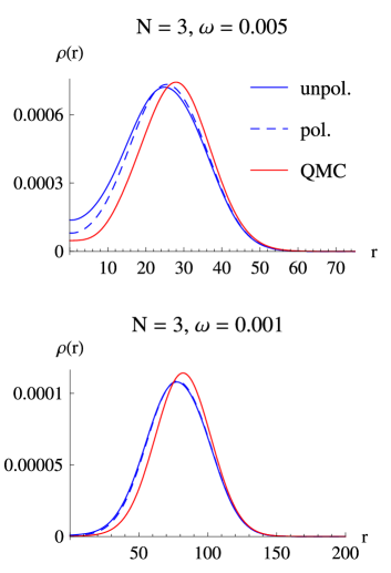
Figure 1: (Color online) Comparison between the densities corresponding to $N=3$ obtained with the KS-SCE approach, both spin-polarized (dashed blue line) and spin-unpolarized (solid blue line) and with spin-polarized Quantum Monte Carlo (red line) from Refs. Ghosal et al., 2006; Guclu et al., 2008.

We have solved the self-consistent Kohn-Sham equations (3) with the SCE potential for different values of the particle number $N$ and the confinement strength $\omega$.

As mentioned, the main objective of this work is to show that KS DFT with the SCE functional is able to capture the features of the strongly-correlated regime without breaking any symmetry. A systematic comparison of the KS-SCE accuracy with available wavefunction results, as well as the optimization of the algorithm, will be the object of future work, where higher-order corrections to the SCE functional will also be developed and tested. Nonetheless, we want to provide an impression for the kind of quantitative accuracy that can be expected from our results. We thus compare, in Fig. 1, the Quantum Monte Carlo densities of Refs. Ghosal et al., 2006; Guclu et al., 2008 for three-electron fully-spin-polarized quantum dots in the strongly-correlated regime with those obtained with our approach (both fully- and non-spin-polarized). It can be seen that already for $\omega=0.005$ the qualitative agreement is rather good, and that there is a small difference between the spin-polarized and unpolarized KS-SCE densities. As the correlation increases with smaller $\omega=0.001$, this difference becomes almost negligible as one would expect, and the agreement between our results and QMC improves. It should be mentioned, however, that in contrast to the QMC calculations at these densities, the KS-SCE energy for the unpolarized cases has slightly lower energy than the spin-polarized solution. We attribute this discrepancy to the fact that the SCE functional, being intrinsically of classical nature, is spin-independent and therefore unable to yield the lowest energy by occupying three different KS orbitals with the same spin. In future works we plan to add magnetic exchange and superexchange corrections to the SCE functional, which should allow the method to recognize the fully-spin-polarized solution as the ground-state one. Quantitatively, the KS-SCE total energy has an error, with respect to QMC, of about 6 mH^∗ ($\sim 6\%$) at $\omega=0.005$ and of about 1 mH^∗ ($\sim 4\%$) at $\omega=0.001$. Notice that, while the fixed-node diffusion Monte Carlo provides an upper bound to the ground-state energy, the KS-SCE self-consistent energies are always a rigorous lower bound to the exact ground-state energy.Malet and Gori-Giorgi (2012); Malet et al. (2013)

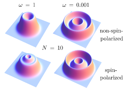
Figure 2: (Color online) Electronic density $\rho(r)$ for a quantum dot with $N=10$ electrons, for $\omega=1$ and $\omega=0.001$.

We now illustrate and discuss the physical features of our results for the electronic densities, going from weakly to strongly-correlated quantum dots. Fig. 2 shows the self-consistent KS-SCE densities for quantum dots with $N=10$ electrons, considering both a strong ($\omega=1$) and a weak ($\omega=0.001$) confinement strength, for the fully-spin-polarized (one electron per Kohn-Sham orbital) and the non-spin-polarized (two electrons per orbital) cases. As mentioned above, when the confinement is strong the quantum dot is in the high-density regime and well described by the fermi-liquid shell structure, with a density distribution qualitatively similar to that obtained from the non-interacting Fock-Darwin states of Eq. (2). Besides some slight oscillations due to the nodal structure of the different orbitals, the resulting densities are rather “thick” or smoothed out, and, particularly in the spin-polarized dot, quite delocalized within the system. In both cases the values of the electron-gas parameter $r_{s}$ are $\simeq 1$.

As the confinement strength becomes weaker, the electron-electron correlation plays an increasingly prominent role. The value $\omega=0.001$ corresponds to extremely low-density quantum dots, with $r_{s}\simeq 68$, significantly larger than the maximum values achieved in previous works using wavefunction methods ($r_{s}\simeq 55$). Guclu et al. (2008) From the figure one can see how the density becomes much sharper in the radial direction, forming two very thin concentric rings centered at the origin. Integration of the density reveals the presence of two electrons in the inner ring and of 8 electrons in the outer one, in agreement with the “8+2” picture of the corresponding classical configuration made up of point-like charges — see table 1 of Ref. Bedanov and Peeters, 1994.

It should be stressed that, as clearly seen from Fig. 2, the densities obtained with the KS-SCE approach correctlyGhosal et al. (2007) preserve the fundamental circular symmetry of the Hamiltonian of Eq. (1). When the $v_{\rm SCE}(\mathbf{r})$ potential, which is constructed from the co-motion functions, is imported into the Kohn-Sham approach, it is able to describe properly the strongly-correlated regime, without introducing any artificial spatial or spin symmetry breaking.

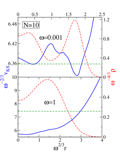
Figure 3: (Color online) Self-consistent Kohn-Sham potentials (blue solid line) and densities (red dashed line) for the strongly- and weakly-correlated unpolarized cases of Fig. 2 (top and bottom, respectively). The green dashed horizontal lines correspond to the energies of the highest occupied KS orbitals. Notice the presence of classically forbidden regions inside the trap in the strongly-correlated case ($\omega=0.001$).

This happens because the SCE exchange-correlation potential self-consistently builds “bumps” that separate the charge density, capturing the physics of charge localization within the non-interacting KS formalism. These structures were already observed in the case of one-dimensional quantum wires using the KS-SCE approach,Malet and Gori-Giorgi (2012); Malet et al. (2013) with each maximum in the density corresponding to a minimum in the Kohn-Sham potential between consecutive “bumps”. In Fig. 3 we show the self-consistent Kohn-Sham SCE potentials for 10-electron quantum dots with $\omega=0.001$ and $\omega=1$. Indeed, in the first case the potential has a local maximum at the origin and a second one in the middle region, giving rise to the density rings of Fig. 2, also reported again in Fig. 3. In particular, the deep second minimum of the KS potential is responsible for the sharp ring of the density in that region. In this way, restricted KS DFT reproduces the effect of strong correlation by means of a local one-body potential. Conversely, in the weakly-interacting case $\omega=1$, the Kohn-Sham potential does not display such structures. Here, the minimum of the density at the origin is not due to any maximum in the potential, but simply results from a fermionic-shell-structure effect. In the same Fig. 3 we also show, as horizontal green dashed lines, the highest occupied KS eigenvalue in both cases. One can clearly see that in the strongly-correlated case ($\omega=0.001$) the barriers in the KS potential create classically forbidden regions inside the trap, giving rise to charge localization.

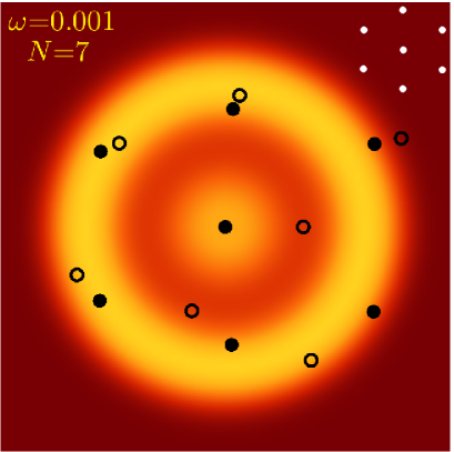
Figure 4: (Color online) Co-motion functions $\mathbf{f}_{i}(\mathbf{r})=(f_{i}(r),\theta_{i}(r))$ for two different configurations of the infinite superposition of Eq. (8), corresponding to the unpolarized dot with $N=7$ and $\omega=0.001$. Empty (solid) symbols represent the co-motion functions for a configuration with a small (large) weight. The classical “1+6” configuration is shown in the top right inset for the sake of comparison. The density is also shown as contour plot, with lighter colors indicating higher density regions.

In order to visualize the internal ordering of the electrons, in wavefunction methods one usually makes use of two-body quantities such as the pair-density distribution,Ghosal et al. (2007) which is not accessible in density-functional approaches. Nevertheless, in the KS-SCE approach this internal ordering can be observed by looking at the co-motion functions of the SCE system, as we illustrate in Fig. 4 for the unpolarized dot with $N=7$ and $\omega=0.001$. The figure shows the co-motion functions $\mathbf{f}_{i}(\mathbf{r})=(f_{i}(r),\theta_{i}(r))$ corresponding to two different configurations, with large and small weight $\rho(r)/N$ in the infinite superposition of Eq. (8), respectively. For this system, the density consists of a peak in the origin (which integrates to one electron) and a sharp ring surrounding it (integrating to six electrons), as illustrated by the superimposed contour plot (lighter colors: higher values of the density). The large-weight configuration is represented by solid symbols, and the low-weight one by empty symbols. In the first case the distribution of the co-motion functions closely resembles the classical point-charge configuration for this system, namely the “6+1” distribution with one charge in the origin surrounded by an hexagon made up of the remaining six charges.Bedanov and Peeters (1994) Notice that in order to yield a smooth density, also unusual configurations (like the one with empty symbols) need to have non-zero weight in the SCE $N$-body density of Eq. (8). However, such configurations have a very small weight in the strongly-correlated regime.

IV.2 Addition energies

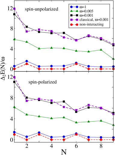
Figure 5: (Color online) Addition energies as a function of $N$, calculated via Eq. (21) from the second difference in total energies, for different values of the confinement strength $\omega$. For comparison, the noninteracting and classical cases are also shown.

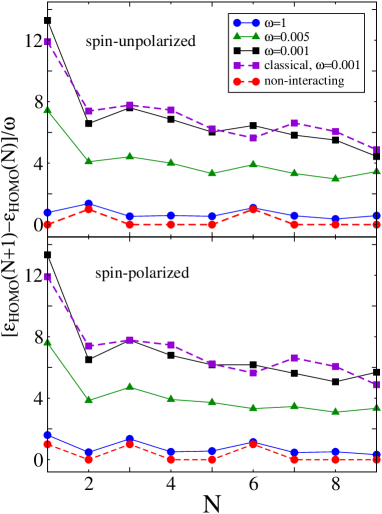
Figure 6: (Color online) Same as Fig. 5, but calculating the addition energies via Eq. (22) from the difference between the Kohn-Sham eigenvalues for the highest occupied orbitals.

In quantum-dot systems, the so-called addition energies provide useful information about the electronic structure of the system and can be probed experimentally.Ashoori (1996); Kouwenhoven et al. (2001) They are defined as the second energy difference

$$E_{\rm add,E}\equiv\Delta_{2}E(N)=E(N+1)-2E(N)+E(N-1)\;,$$ (21)

where $E(N)$ is the total energy for the $N$-electron quantum dot. For KS DFT calculations, one can also use the alternative expression

$$E_{\rm add,HO}=\varepsilon_{\rm HO}(N+1)-\varepsilon_{\rm HO}(N)\;.$$ (22)

It results from the fact that in the exact KS theory — that is, if the exact exchange-correlation potential were used — the highest occupied (HO) Kohn-Sham eigenvalue $\varepsilon_{\rm HO}(N)$ is equal to minus the ionization energy of the physical, interacting, $N$-electron system,Almbladh and von Barth (1985); Levy et al. (1984) i.e., $\varepsilon_{\rm HO}(N)=E(N)-E(N-1)$. Notice that whereas the calculation of the addition energies using Eq. (21) requires knowledge about three different systems, the second alternative formula of Eq. (22) only involves two of them. When using approximate functionals, the two expressions will not, in general, give the same results.

Figures 5 and 6 show the KS-SCE addition energies for quantum dots with up to $10$ electrons computed via Eq. (21) and Eq. (22), respectively, for different strengths of the confining potential. From both figures one can see that for strong confinement ($\omega=1$) the addition energies are qualitatively similar to the non-interacting ones. In particular, for the non-spin-polarized systems they show the well-known peaks at $N=2$ and 6, corresponding to the closure of the first ($m=0$) and second ($m=\pm 1$) shells, and also the smaller peak at $N=4$ due to Hund’s rule. In the spin-polarized case, instead, the peaks are found at $N=1$ (first shell, $m=0$), at $N=3$ (second shell, $m=\pm 1$) and at $N=5$ (third shell, $m=\pm 2$). When the quantum dots become strongly correlated, the shell structure changes radically. The first main well-known feature is a flattening of the addition spectrum (notice that in the figure the energies are divided by $\omega$, which in the low-density cases takes values as low as $0.005$ and $0.001$). Secondly, the peak sequence becomes more irregular and resembles qualitatively the equivalent classical point-charge system.Guclu et al. (2008)

V Conclusions and Perspectives

We have demonstrated the feasibility of constructing an exchange-correlation potential for spin-restricted Kohn-Sham density functional theory which is able to describe strong correlation effects in two-dimensional model quantum dots. This functional is derived from the exact properties of the strong-coupling limit of the Hohenberg-Kohn functional. It allows us to treat low-density quantum dots at relatively low computational cost when compared to other commonly employed approaches for studying these systems. Notice that, already for the number of particles and at the low densities considered here, CI calculations are not feasible. In the case of QMC, one has needed, so far, to make use of orbitals localized on different sites, thus breaking the circular symmetry of the system.Guclu et al. (2008) Our approach is numerically much less expensive, providing access to a broader parameter range than before. It also yields a set of radically new KS orbitals, which could be used in QMC instead of the localized gaussian ones. In other words, it would be very interesting to see if the KS-SCE orbitals provide good nodes for fixed-node diffusion Monte Carlo at low densities, avoiding the need of breaking the circular symmetry.Reinhardt et al. (2012)

Overall, this new methodology shows the promise of becoming a powerful tool in low-dimensional, low-density, electronic structure calculations. To exploit its full potential, several issues still need to be addressed in future works. First of all, corrections need to be designed to take the effects of the spin state in the SCE functional into account, for example using approximate magnetic exchange and superexchange functionals. Secondly, an efficient algorithm to solve (exactly or in a reasonably approximate way) the SCE equations for general (non-circularly symmetric) geometry needs to be fully developed. A viable route for this seems to be the dual Kantorovich formulation of the SCE functional,Buttazzo et al. (2012) whose first pilot implementationMendl and Lin (2013) has given promising results.

Acknowledgments

We thank Cyrus Umrigar and Devrim Guclu for the QMC densities of the $N=3$ quantum dots and for interesting discussions. C.B.M. acknowledges support from the DFG project FR 1275/3-1. P.G-G. acknowledges support from the Netherlands Organization for Scientific Research (NWO) through a Vidi grant. Finally, this research was supported by a Marie Curie Intra European Fellowship within the 7th European Community Framework Programme (F.M.).

References

- Ghosal et al. (2006) A. Ghosal, A. D. Guclu, C. J. Umrigar, D. Ullmo, and H. U. Baranger, Nature Phys. 2, 336 (2006).
- Guclu et al. (2008) A. D. Guclu, A. Ghosal, C. J. Umrigar, and H. U. Baranger, Phys. Rev. B 77, 041301 (2008).
- Yannouleas and Landman (2007) C. Yannouleas and U. Landman, Rep. Prog. Phys. 70, 2067 (2007).
- Auslaender et al. (2005) O. M. Auslaender, H. Steinberg, A. Yacoby, Y. Tserkovnyak, B. I. Halperin, K. W. Baldwin, L. N. Pfeiffer, and K. W. West, Science (New York, N.Y.) 308, 88 (2005).
- Kristinsdottir et al. (2011) L. H. Kristinsdottir, J. C. Cremon, H. A. Nilsson, H. Q. Xu, L. Samuelson, H. Linke, A. Wacker, and S. M. Reimann, Phys. Rev. B 83, 041101 (2011).
- Creffield et al. (1999) C. E. Creffield, W. Hausler, J. H. Jefferson, and S. Sarkar, Phys. Rev. B 59, 10719 (1999).
- Egger et al. (1999) R. Egger, W. Hausler, C. H. Mak, and H. Grabert, Phys. Rev. Lett. 82, 3320 (1999).
- Yannouleas and Landman (1999) C. Yannouleas and U. Landman, Phys. Rev. Lett. 82, 5325 (1999).
- Reimann et al. (2000) S. Reimann, M. Koskinen, and M. Manninen, Phys. Rev. B 62, 8108 (2000).
- Filinov et al. (2001) A. V. Filinov, M. Bonitz, and Y. E. Lozovik, Phys. Rev. Lett. 86, 3851 (2001).
- Pederiva et al. (2002) F. Pederiva, A. Emperador, and E. Lipparini, Phys. Rev. B 66, 165314 (2002).
- Ghosal et al. (2007) A. Ghosal, A. D. Guclu, C. J. Umrigar, D. Ullmo, and H. U. Baranger, Phys. Rev. B 76, 085341 (2007).
- Wigner (1934) E. P. Wigner, Phys. Rev. 46, 1002 (1934).
- Weiss et al. (2006) S. Weiss, M. Thorwart, and R. Egger, Europhys. Lett. 76, 905 (2006).
- Deshpande and Bockrath (2008) V. V. Deshpande and M. Bockrath, Nature Phys. 4, 314 (2008).
- Taylor and Calarco (2008) J. M. Taylor and T. Calarco, Phys. Rev. A 78, 062331 (2008).
- Ballester et al. (2010) A. Ballester, J. M. Escartín, J. L. Movilla, M. Pi, and J. Planelles, Phys. Rev. B 82, 115405 (2010).
- Reimann and Manninen (2002) S. M. Reimann and M. Manninen, Rev. Mod. Phys. 74, 1283 (2002).
- Rontani et al. (2006) M. Rontani, C. Cavazzoni, D. Bellucci, and G. Goldoni, J. Chem. Phys. 124, 124102 (2006).
- Waltersson et al. (2013) E. Waltersson, C. J. Wesslén, and E. Lindroth, Phys. Rev. B 87, 035112 (2013).
- Stoudenmire et al. (2012) E. Stoudenmire, L. O. Wagner, S. R. White, and K. Burke, Phys. Rev. Lett. 109, 056402 (2012).
- Borgh et al. (2005) M. Borgh, M. Toreblad, M. Koskinen, M. Manninen, S. Aberg, and S. M. Reimann, Int. J. Quantum Chem. 105, 817 (2005).
- Anisimov et al. (1991) V. I. Anisimov, J. Zaanen, and O. K. Andersen, Phys. Rev. B 44, 943 (1991).
- Harju et al. (2004) A. Harju, E. Räsänen, H. Saarikoski, M. J. Puska, R. M. Nieminen, and K. Niemelä, Phys. Rev. B 69, 153101 (2004).
- Hohenberg and Kohn (1964) P. Hohenberg and W. Kohn, Phys. Rev. 136, B 864 (1964).
- Kohn and Sham (1965) W. Kohn and L. J. Sham, Phys. Rev. A 140, 1133 (1965).
- Cohen et al. (2008) A. J. Cohen, P. Mori-Sanchez, and W. T. Yang, Science 321, 792 (2008).
- Abedinpour et al. (2007) S. H. Abedinpour, M. Polini, G. Xianlong, and M. P. Tosi, Eur. Phys. J. B 56, 127 (2007).
- Zeng et al. (2009) L. Zeng, W. Geist, W. Y. Ruan, C. J. Umrigar, and M. Y. Chou, Phys. Rev. B 79, 235334 (2009).
- Malet and Gori-Giorgi (2012) F. Malet and P. Gori-Giorgi, Phys. Rev. Lett. 109, 246402 (2012).
- Malet et al. (2013) F. Malet, A. Mirtschink, J. C. Cremon, S. M. Reimann, and P. Gori-Giorgi, Phys. Rev. B 87, 115146 (2013).
- Seidl et al. (2007) M. Seidl, P. Gori-Giorgi, and A. Savin, Phys. Rev. A 75, 042511 (2007).
- Gori-Giorgi et al. (2009a) P. Gori-Giorgi, M. Seidl, and G. Vignale, Phys. Rev. Lett. 103, 166402 (2009a).
- Gori-Giorgi and Seidl (2010) P. Gori-Giorgi and M. Seidl, Phys. Chem. Chem. Phys. 12, 14405 (2010).
- Buijse et al. (1989) M. A. Buijse, E. J. Baerends, and J. G. Snijders, Phys. Rev. A 40, 4190 (1989).
- Helbig et al. (2009) N. Helbig, I. V. Tokatly, and A. Rubio, J. Chem. Phys. 131, 224105 (2009).
- Jacak et al. (1998) L. Jacak, P. Hawrylak, and A. Wójs, Quantum Dots (Springer, Berlin, 1998).
- Seidl (1999) M. Seidl, Phys. Rev. A 60, 4387 (1999).
- Seidl et al. (1999) M. Seidl, J. P. Perdew, and M. Levy, Phys. Rev. A 59, 51 (1999).
- Seidl et al. (2000) M. Seidl, J. P. Perdew, and S. Kurth, Phys. Rev. Lett. 84, 5070 (2000).
- Buttazzo et al. (2012) G. Buttazzo, L. De Pascale, and P. Gori-Giorgi, Phys. Rev. A 85, 062502 (2012).
- Cotar et al. (2013) C. Cotar, G. Friesecke, and C. Klüppelberg, Comm. Pure Appl. Math. 66, 548 (2013).
- Gori-Giorgi et al. (2009b) P. Gori-Giorgi, G. Vignale, and M. Seidl, J. Chem. Theory Comput. 5, 743 (2009b).
- Mirtschink et al. (2012) A. Mirtschink, M. Seidl, and P. Gori-Giorgi, J. Chem. Theory Comput. 8, 3097 (2012).
- Bedanov and Peeters (1994) V. M. Bedanov and F. M. Peeters, Phys. Rev. B 49, 2667 (1994).
- Ashoori (1996) R. C. Ashoori, Nature 379, 413 (1996).
- Kouwenhoven et al. (2001) L. P. Kouwenhoven, D. G. Austing, and S. Tarucha, Rep. Prog. Phys. 64, 701 (2001).
- Almbladh and von Barth (1985) C.-O. Almbladh and U. von Barth, Phys. Rev. B 31, 3231 (1985).
- Levy et al. (1984) M. Levy, J. P. Perdew, and V. Sahni, Phys. Rev. A 30, 2745 (1984).
- Reinhardt et al. (2012) P. Reinhardt, J. Toulouse, R. Assaraf, C. J. Umrigar, and P. E. Hoggan, ACS Symposium Series 53, 1094 (2012).
- Mendl and Lin (2013) C. B. Mendl and L. Lin, Phys. Rev. B 87, 125106 (2013).