Exact and approximate solutions for the quantum minimum-Kullback-entropy estimation problem

Abstract

The minimum Kullback entropy principle (mKE) is a useful tool to estimate quantum states and operations from incomplete data and prior information. In general, the solution of a mKE problem is analytically challenging and an approximate solution has been proposed and employed in different context. Recently, the form and a way to compute the exact solution for finite dimensional systems has been found, and a question naturally arises on whether the approximate solution could be an effective substitute for the exact solution, and in which regimes this substitution can be performed. Here, we provide a systematic comparison between the exact and the approximate mKE solutions for a qubit system when average data from a single observable are available. We address both mKE estimation of states and weak Hamiltonians, and compare the two solutions in terms of state fidelity and operator distance. We find that the approximate solution is generally close to the exact one unless the initial state is near an eigenstate of the measured observable. Our results provide a rigorous justification for the use of the approximate solution whenever the above condition does not occur, and extend its range of application beyond those situations satisfying the assumptions used for its derivation.

I Introduction

Let us consider a situation where a quantum system is prepared in a known state and , after some time and unknown evolution, some measurements are performed in order to gather information on the final state. The exact solution to this state estimation problem is provided by quantum tomography, which however requires the measurement of a complete set (i.e. a quorum) of observables Dar01 .

Measuring a quorum of observables may be experimentally challenging, or require too many resources, and therefore it is worth exploring the case where the set of observables that can be measured on the system is incomplete LNP . In this case, we cannot obtain complete information about the state of the system from the outcomes of these measurements, i.e. the measurements are not fully determining the state of the system. We thus need some additional ingredient to fill the information gap and single out a quantum state that is compatible with the data, and with the information that is possibly available prior to the measurements zhr97 ; zhr00 .

When we have no a priori information, e.g. because the initial state of the system is unknown or the interaction with the environment is strong enough to wash out any initial information, the problem may be attacked using the maximum entropy principle (ME) Jaynes ; rmp13 . With the ME we take all the states (density matrices) compatible with the evidences, i.e. reproducing the correct probabilities of the observed data, and pick up the one maximizing the Von Neumann entropy. In this way, the only knowledge about the state is that coming from the measurements made on the system, without the addition of any unwanted piece of extra information which is not available from the experimental evidences Buz97 ; Zim08 .

On the other hand, there are several situation of interest where some a priori information is indeed available, in the form of a a priori state. This may be due to some constraints imposed to the physical preparation of the system, or to the fact that the coupling of the system with the rest of the universe is weak, so that the state remains close to the initial preparation. In these cases, the minimum Kullback entropy (mKE) principle Kull51 ; Shore80 provides an effective tool to include this new ingredient in the solution and to complement the experimental data, thus allowing to obtain a unique estimated state.

The mKE principle has received attention in the recent years and has been applied to both finite and infinite-dimensional systems Geo06 ; Oli07 ; Tic10 ; Zor11 . In particular, applications to qubit and harmonic oscillator systems have been initially put forward upon exploiting an approximate solution of the minimization problem Oli07 ; Oli12 . More recently, the analysis of the feasibility, the form of the general solution and a method to compute it has been derived for finite dimensional systems Ticozzi and a question naturally arises on how the approximate solution compares to the exact one, and in which regimes it could be convenient to employ the former. Indeed, our analysis is motivated by two relevant properties of the approximate solution: on the one hand it is given in a closed form which is more convenient for applications and, on the other hand, it may be applied to a larger class of a priori states, including those described by a density operator not having full rank.

This paper focuses on qubit systems in situations where only the average of a single observable can be accessed. We consider the use of mKE for estimation of states and for the characterization of weak Hamiltonians, and compare the two solutions in terms of state fidelity and operator distance respectively. We find that the approximate solution is generally close to the exact one unless the initial state is near an eigenstate of the measured observable. Our results thus provide a rigorous justification for the use of the approximate solution whenever the above condition does not occur.

The paper is structured as follows. In Sec. II we review the mKE principle for a qubit system where a single observable is measured, and present both the approximate and the exact solutions to the mKE estimation problem. In Sec. III a systematic comparison between the approximate and the exact solution is performed in terms of fidelity, and the role of initial purity is discussed. In Sec. IV we address estimation of weak Hamiltonians by mKE and compare the approximate and the exact solutions in terms of operator trace distance. Sec. V closes the paper with some concluding remarks.

II The minimum Kullback entropy principle

The quantum Kullback (Umegaki’s) relative entropy between two quantum states is defined as Umegaki ; Pet91 ; Hay01 ; Ved02 :

$$K(\rho|\tau)=\mathrm{Tr}\left[{\rho(\log\;\rho-\log\;\tau)}\right]\,.$$ (1)

As for its classical counterpart, the Kullback-Leiber divergence, it can be demonstrated that $0\leq K(\rho|\tau)<\infty$ when it is definite, i.e. when the support of the first state in the Hilbert space is contained in that of the second one. In particular, $K(\rho|\tau)=0$ iff $\rho\equiv\tau$. This quantity, though not defining a proper metric in the Hilbert space (it is not simmetric in its arguments), has been widely used in different fields of quantum information Ved02 ; Sch02 ; Gal00 ; Qin08 ; ng1 ; ng2 because of its additivity properties and statistical meaning in state discrimination.

Let us now consider a quantum system initially prepared in the state $\tau$ that, after some kind of evolution, unitary or not, is now in the final state $\rho$. In this case we have some prior information that we can regard as a bias towards $\tau$. Furthermore, when some observables are measured, the information achieved (e.g. their mean values or their full probability distributions) gives some constraints about the state. The mKE principle, states that the best estimate for the state $\rho$ is then the density matrix that satisfies the constraints and, at the same time, is somehow closer to the initial state $\tau$, i.e. minimize the quantum Kullback entropy, given the constraints. The mKE principle allows one to take into account the available prior information as well as the new evidence coming from the data, while not introducing any other kind of spurious or unwanted piece of information.

The minimization can be done by Lagrange multipliers. If the constraint is given by the mean value of the observable $A$ (and by the normalization), then the quantity that should be minimized is:

$$F(\rho,\lambda_{1},\lambda_{2})=K(\rho|\tau)\; +\lambda_{1}(\mathrm{Tr}\left[{\rho}\right]-1)$$

$$+\lambda_{2}(\mathrm{Tr}\left[{\rho A}\right]-\langle A\rangle),$$ (2)

$\lambda_{k}$ being the Lagrange multipliers. Two approaches have been developed to solve this mKE problem. The first is approximate and leads to analytic solutions in several cases, e.g. when the final state is close to the initial one Bra96 ; Oli07 . More recently, the general feasibility of this estimation problem and an exact method has been developed, valid when the quantum system under investigation is finite dimensional Ticozzi . Having at disposal an exact solution allows us to assess the approximate one and to individuate the situations where it may safely apply instead of the exact one. In the following we are going to systematically compare the two solutions for a qubit system subjected to the measurement of a single observable.

II.1 General Solution

It is possible to show that, for finite-dimensional Hilbert spaces, the minimum of the Eq. (II) exists, is unique and continuous with respect to the data Ticozzi . After a suitable reduction of the problem to a subspace that ensures that the solution is full rank, and assuming that $\tau$ is full-rank on the same subspace, the optimal solution of the problem, when the only outcome of the measurement is the mean value of observable $A$, is the following one:

$$\rho(\lambda_{1},\lambda_{2})=e^{\log{\tau}-\mathbb{I}-\lambda_{1}X_{1}-\lambda_{2}X_{2}}$$ (3)

where $\lambda_{1}$, $\lambda_{2}$ are Lagrange multipliers, and $X_{1}$, $X_{2}$ are the operators obtained from $\mathbb{I}$ and $A$ through the Gram-Schmidt orthogonalization process. Notice that if $\tau$ is not full rank the above formula does not return a valid density operator. In order to evaluate the Lagrange multipliers, the constraints of normalization $\hbox{Tr}[\rho(\lambda_{1},\lambda_{2})]=1$ and mean value of $A$, $\hbox{Tr}[\rho(\lambda_{1},\lambda_{2})\,A]=\langle A\rangle$ should be imposed.

II.2 Approximate solution

Assuming that the evolution is not leading the system too far away from its initial preparation, we can find an approximate solution to the mKE estimation problem upon writing the infinitesimal increment of the density operator. More explicitly: in the Hilbert space of statistical operators, one considers an infinitesimal increment of the operator $\rho$ correspoding to the increment of an arbitrary parameter $\lambda$. Upon assuming that increments of the density operator are evaluated according to the Fisher metric it is possible to introduce the differential equation Bra96 :

$$\frac{d\rho}{d\lambda}=-\frac{1}{2}\{\rho,A-\langle A\rangle\}$$ (4)

where $\{\ ,\ \}$ is the anticommutator. As already mentioned, the same equation can be obtained from Eq. (II), when the final state $\rho$ is close to the initial state $\tau$, according to the Fisher metric. In turn, the state $\rho$ obtained by integration of Eq. (4) is the approximate solution of the mKE problem with $\lambda$ playing the role of a Lagrange multiplier.

This work focuses on statistical operator in the qubit space, when the initial state is given and the only information obtained from measurement is the mean value of the observable $A$. The solution of the previous equation for this case (notice that it is also correct for spaces with dimension larger than two) is:

$$\rho(\lambda)=\frac{e^{-A\lambda/2}\tau e^{-A\lambda/2}}{\mathrm{Tr}\left[{\tau e^{-A\lambda}}\right]}$$ (5)

where $\lambda$ can be found using the constraint $\mathrm{Tr}\left[{A\rho}\right]=\langle A\rangle$. As mentioned above, the approximate solution $\rho(\lambda)$ may be computed also if $\tau$ is not full rank. In addition, we notice that $\rho(\lambda)$ has the same rank of the a priori state $\tau$.

Since the approximate solution has been derived assuming that evolved state is close to the initial one Bra96 , one may expect that $\rho(\lambda)$ obtained from Eq. (5) is not too far away from the a priori state $\tau$. As we will show in the following, this is basically true in the case of nearly pure initial states. Otherwise, when the initial state is appreciably mixed, the approximate solution can, in fact, be far away from the initial preparation. On the other hand, also in these cases the approximate solution is close to the exact one. In other words, having at disposal the exact solution allows us to assess the approximate one also outisde the assumptions made to derive it, and to extend the regimes where it may be safely employed.

III Comparison between the exact and the approximate mKE estimates

In this section the two solutions are compared, through the use of the fidelity, in order to establish whether, and in which conditions, the approximate solution can be considered as a good replacement for the exact one. The comparison is made for qubits systems.

In particular, we address situations where a single observable $A$ is measured. The most general qubit observable may be written as

$$A=a_{0}\mathbb{I}+{\boldsymbol{a}}\cdot\boldsymbol{\sigma}\,,$$

where $a_{0}$ and $\boldsymbol{a}=(a_{1},a_{2},a_{3})$ are real parameters and $\boldsymbol{\sigma}=(\sigma_{1},\sigma_{2},\sigma_{3})$ denote the Pauli matrices vector. Without loss of generality it is always possible to perform a rotation and a scaling in order to rewrite the observable as

$$U^{\dagger}\,A\,U=A=\alpha\mathbb{I}+\sigma_{3}$$ (6)

i.e. as a function of a single real parameter $\alpha$.

Once the rotation is made, we rewrite the general state of the qubit in the new reference as

$$\tau=\frac{1}{1+\epsilon}(\left|{\psi}\right\rangle\left\langle{\psi}\right|+\epsilon\left|{\psi^{\perp}}\right\rangle\left\langle{\psi^{\perp}}\right|)\,,$$

where

$$\left|{\psi}\right\rangle=\cos{\frac{\theta}{2}}\left|{0}\right\rangle+e^{i\phi}\sin{\frac{\theta}{2}}\left|{1}\right\rangle$$

is the generic pure state and $\left|{\psi^{\perp}}\right\rangle$ its orthogonal complement. The parameter $\epsilon$ depends on the purity $\mu[\tau]$ of the initial state $\tau$, we have:

$$\mu[\tau]=\frac{1+\epsilon^{2}}{(1+\epsilon)^{2}}\,,$$

with $\mu\in[1/2,1]$.

The parameters involved in this problem are five. The three parameters $\theta\in[0,\pi]$, $\phi\in[0,2\pi)$ and $\mu\in[1/2,1]$ are needed to fully characterize the initial state, whereas $\alpha\in\mathbb{R}$ and $\langle\sigma_{3}\rangle\in[-1,1]$ specify the measured observable and its mean values respectively: $\langle A\rangle=\alpha+\langle\sigma_{3}\rangle$. Since we are dealing with qubit measurements (which have two possible outcomes) the knowledge of the mean value is equivalent to that of the full distribution.

Once we fix both $\tau$ and $A$, the approximate and exact solutions can be evaluated using, respectively, Eq. (5) and Eq. (3). The approximate solution in Eq. (5) has an analytic form, which is independent of $\alpha$, and is given by Oli07

$$\rho(\lambda)=\frac{e^{-\frac{1}{2}\lambda\sigma_{3}}\,\tau\,e^{-\frac{1}{2}\lambda\sigma_{3}}}{\hbox{Tr}[\tau\,e^{-\lambda\sigma_{3}}]}\,,$$ (7)

where $\lambda$ is determined by solving the equation $\hbox{Tr}[\rho(\lambda)\,\sigma_{3}]=\langle\sigma_{3}\rangle$. The analytic form of the Bloch vector ${\boldsymbol{r}}=(r_{1},r_{2},r_{3})$ of $\rho(\lambda)=\frac{1}{2}\left({\mathbb{I}}+{\mathbf{r}}\cdot{\boldsymbol{\sigma}}\right)$ is given by:

$$r_{1}=\frac{t_{1}}{Z}\ ;\ r_{2}=\frac{t_{2}}{Z}\ ;\ r_{3}=\langle\sigma_{3}\rangle$$

where ${\boldsymbol{t}}=(t_{1},t_{2},t_{3})$ is the Bloch vector of the initial state $\tau$ and $Z=\cosh{\lambda}-t_{3}\sinh{\lambda}$ (see Appendix A for the explicit expression in terms of the parameters $\theta$, $\phi$, and $\epsilon$). The corresponding value of the Lagrange multiplier is

$$\lambda=\mathrm{arctanh}\frac{t_{3}-\langle\sigma_{3}\rangle}{1-\langle\sigma_{3}\rangle t_{3}}\,.$$ (8)

For what concerns the optimal solution, the first Lagrange multiplier $\lambda_{1}$ is evaluated using the trace normalization for the state $\rho$, while the second one $\lambda_{2}$ is evaluated upon exploiting the constraint of the mean value. The equation for the last constraint is transcendental, and numerical methods are needed in order to find $\lambda_{2}$. When the values of the two solutions are found, for fixed $\tau$ and $A$, it is possible to compare them using the qubit fidelity:

$$F(\rho_{1},\rho_{2})=\mathrm{Tr}\left[{\rho_{1}\rho_{2}}\right]+\sqrt{1-\mu[\rho_{1}]}\sqrt{1-\mu[\rho_{2}]}$$ (9)

where $\mu[\rho_{k}]$ is the purity of the state $\rho_{k}$, $\rho_{1}$ is the approximate solution and $\rho_{2}$ the exact one.

In order to assess the reliability of the approximate solution we have evaluated the fidelity between the approximate and the exact solution as a function of the five parameters involved in the estimation problem. Our first result is that the fidelity does not depend on the angle $\phi$, i.e. the two solutions (approximate and exact) show the same functional dependence on such parameter. Besides, the approximate and the exact mKE estimate, as well as the fidelity, do not depend on the parameter $\alpha$.

The relevant parameters to assess the approximate solution are thus the angle polar $\theta$ and the purity $\mu[\tau]$ of the initial state and the result of the measurement $\langle\sigma_{3}\rangle$. The fidelity is also symmetric with respect to the transformations $\theta\rightarrow\pi-\theta$ and $\langle\sigma_{3}\rangle\rightarrow-\langle\sigma_{3}\rangle$. Notice that finding the exact mKE solution requires the use of numerical methods, which pose a upper bound to the initial purity $\mu[\tau]\lesssim 1-10^{-7}$, above which the solution becomes numerically unstable.

As we will see in the following, the fidelity shows different behaviors, depending on the purity $\mu[\tau]$ of the initial state $\tau$. Before going to a detailed comparison, we notice that if the initial state $\tau$ commutes with the measured observable $A$, i.e. $[\tau,A]=0$, then the two solutions coincide as it is apparent by inspecting Eq. (3) and Eq. (5).

III.1 Fidelity for highly mixed initial states

When the purity $\mu$ of the initial state takes values between $1/2$ and, say, $0.9$ (i.e. when the initial state is highly mixed), the fidelity presents some distinctive features, highlighted in Fig. 1.

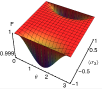
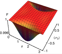
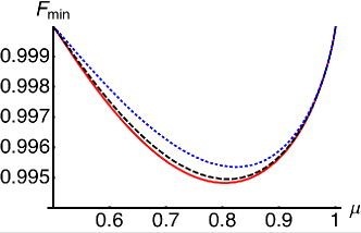
Figure 1: (Color online) Fidelity between the exact and the approximate mKE estimate as a function of the parameter $\theta$ of the initial state and of the outcome of the measurement $\langle\sigma_{3}\rangle$. The plots are for two fixed values of the initial purity: $\mu=0.55$ (top left) and $\mu=0.7$ (top right). The lower panel shows the minimum of fidelity for $\theta=\pi/2$ (solid red), $\theta=5\pi/12$ (black dashed), $\theta=\pi/3$ (blue dotted) as a function of purity $\mu$.

As it is apparent from the plots, the fidelity between the two solutions is extremely close to unit for a large range of values of $\langle\sigma_{3}\rangle$ around $\langle\sigma_{3}\rangle=0$, whereas for values of $\langle\sigma_{3}\rangle$ near $\pm 1$ it decreases and shows a minimum. The shape is almost independent on the value of the initial purity, whereas the minimal value does. The actual value of the minimum also depends on the angle $\theta$ and the global minimum is achieved for $\theta=\pi/2$. It is worth noticing that the values of these minima corresponds to fidelity always larger than $F=0.995$, i.e. the two estimates are very close each other anyway nota .

The values of the global minimum as a function of purity, is reported in the lower panel of Fig. 1. Notice that when the purity of the state $\tau$ tends to $1/2$, i.e. the initial state approaches $\tau=\mathbb{I}/2$, the two solutions coincides for all values of $\theta$ and $\langle\sigma_{3}\rangle$, as it may readily seen from Eq. (3) and Eq. (5). This corresponds to the case of a system initially in a maximally mixed state and for which the measurement is not providing any additional information. The minimum of the fidelity between the two estimates is observed for $\mu\simeq 0.8$ and then, for increasing purity, the two solutions become again very close each other.

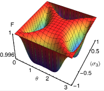
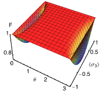
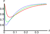
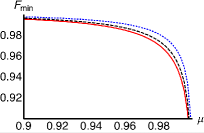
Figure 2: (Color online) Fidelity between the exact and the approximate mKE estimate for $\mu=0.9$ (left) and $\mu=0.9999$ (right). The lower left panel shows the behavior of the fidelity as a function of $\theta$ for $\langle\sigma_{3}\rangle=0$ and for different (close to unit) values of purity: $\mu=1-10^{-4}$ (solid red line), $\mu=1-10^{-5}$ (green dashed), $\mu=1-10^{-6}$ (blue dotted). The lower right panel shows the minimum of fidelity for for $\langle\sigma_{3}\rangle=0$ (solid red line), $\langle\sigma_{3}\rangle=\pm 0.3$ (black dashed), $\langle\sigma_{3}\rangle=\pm 0.5$ (blue dotted).

III.2 Fidelity for nearly pure initial states

Let us now analyze the situation in which the initial state $\tau$ is closer to a pure state, with $\mu\in[0.9,1]$. In this regime, the fidelity presents a behavior which is quite different from the one illustrated in the previous Section. In particular, the minima seen for $\theta$ around $\pi/2$ and $|\langle\sigma_{3}\rangle|\rightarrow 1$ disappear and are replaced by minima occurring for $\theta$ close to $0$ or $\pi$ and for $\langle\sigma_{3}\rangle=0$. These phenomena are illustrated in the upper panels of Fig. 2, where we report the behavior of fidelity as a function of $\theta$ and $\langle\sigma_{3}\rangle$ for two values of the initial purity. The plot for $\mu=0.9$ still shows the two kinds of minima, whereas for larger values the transition from a regime to the other is completed.

As it is apparent from Fig. 2, the exact and approximate estimates almost coincide for most values of $\theta$ and $\langle\sigma_{3}\rangle$, while their fidelity starts to differ from unit when $\theta$ is near $0$ or $\pi$. The discrepancy becomes more and more appreciable as far as $\langle\sigma_{3}\rangle$ approaches $0$. Another information extracted from these plots is that the range of $\theta$ values where the fidelity is appreciably smaller than one tends to shrink and move towards zero while the purity increases. In other words, when $\mu\rightarrow 1$, and therefore the initial state $\tau$ is pure, the minimum of fidelity stays on $\theta=0$,$\pi$, while for all the other values of $\theta$ and $\langle\sigma_{3}\rangle$ the exact and the approximate mKE solutions coincide. When the purity of the initial state decreases (still being larger than a threshold value, say 0.9), we find a neighborhood of $\theta=0$ (and $\pi$) where the two solutions are different. Furthermore, in this interval of $\theta$ values, the fidelity decreases towards a minimum, which approaches to $1/2$ (the two states are completely unrelated) when $\mu$ goes to unit.

The lower right panel of Fig. 2 shows the behavior of the global minimum as a function of purity. Notice that for a nearly pure initial state, the values taken by the fidelity in the minimum may be far from one. This behavior may be understood as follows: let us consider the point of minimum fidelity, i.e. $\theta=0$ (or $\pi$) and $\langle\sigma_{3}\rangle=0$, for $\mu\rightarrow 1$. This corresponds to assume the initial state $\tau$ to be one of the pure, $\left|{0}\right\rangle$ or $\left|{1}\right\rangle$, eigenstates of $\sigma_{3}$. On the other hand, if the measured mean value of $\sigma_{3}$ is zero this suggest that the state $\rho$ is somehow mixed. In fact, the exact mKE estimate is the completely mixed state $\rho\simeq\mathbb{I}/2$. On the contrary, the approximate solution is the pure state $\left|{\phi}\right\rangle=1/\sqrt{2}(\left|{0}\right\rangle+\left|{1}\right\rangle)$. In other words, the very form of the approximate solution tends to keep the purity of the initial state unchanged, as it is apparent from Eq. (5) when we consider $\tau=\left|{\psi}\right\rangle\left\langle{\psi}\right|$.

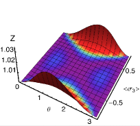
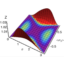
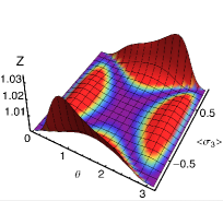
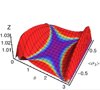
Figure 3: (Color online) The ratio, $Z$, between the two fidelities $F(\rho_{apx},\tau)$ and $F(\rho_{exa},\tau)$, as a function of $\theta$ and $\langle\sigma_{3}\rangle$, for different values of initial purity $\mu$. In the first graphic we have $Z$ for $\mu=0.7$. Then, from top to bottom, from left to right, we find graphics for $\mu=0.8$, $\mu=0.9$ and $\mu=0.99$. It is evident that $Z$ is always greater (or equal) than one, which means that $\rho_{apx}$ is, in general, closer to $\tau$ than $\rho_{exa}$.

Actually, the approximate method appears to force the solution to be closer to the initial state than the exact solution of Eq. (3) does, in agreement with the assumptions used for its derivation. More precisely, the approximate solution is closer, in terms of fidelity, to the initial state than the exact one, for any values of $\mu$, $\theta$ and $\langle\sigma_{3}\rangle$. This phenomenon is illustrated in Fig. 3, where we report the ratio $Z=F(\rho_{apx},\tau)/F(\rho_{exa},\tau)$ between the fidelities of the two solution to the initial state. As it is apparent from the plots, we have $Z\geq 1$ for the whole range of parameters and, in turn, this confirms the above considerations.

It is worth to notice that both the relative entropy and the fidelity can be used to measure the similarity between two quantum states. Since the mKE principle minimizes the Kullback entropy, the exact solution should be closer to the initial state than the approximate one in terms of relative entropy, whereas ther are no constraints on the fidelity. Overall, our results shows that, in this case, fidelity and relative entropy provides two opposite assessments nota .

III.3 The purity of the two solutions

As we have seen in the previous Sections, when the initial state shows high purity the approximate solutions tends to preserve such purity irrespective of the results of the measurements, whereas this is not the case for the exact solution. Since this phenomenon represents the underlying reason of the behavior of fidelity reported in the previous Section, here we provide a more detailed study of the purity of the exact and approximate solutions as functions of the purity $\mu$ of the initial state $\tau$.

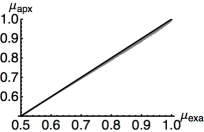
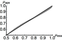
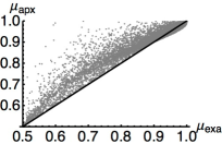
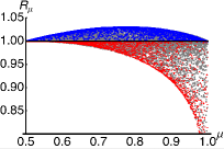
Figure 4: (Color online) Purities of the approximate and exact solutions of mKE estimation. The first three plots show the purity of the approximate solutions as a function of the exact one for the initial purity in the ranges $\mu=0.5-0.6$ (top left), $\mu=0.7-0.8$ (top right) and $\mu=0.9-1.0$ (down left) respectively. In all the plots grey points correspond to purities of mKE solutions obtained by random selecting the initial states with $\theta\in[0,\pi]$ and $\mu$ in the given range, and simulating random measurements with $\langle\sigma_{3}\rangle\in[-1,1]$. The right lower panels shows the ratio $R_{\mu}$ as function of initial purity $\mu$. Here the grey points are obtained by randomly selecting the initial states in the full range of $\theta$ and $\mu$ and $\langle\sigma_{3}\rangle\in[-1,1]$, the blue (square) points are obtained by sampling $\theta$ in the range $\theta\in[\pi/2-\pi/10,\pi/2+\pi/10$ and $|\langle\sigma_{3}\rangle|\in[0.9,1]$, and the red (rhombus) points correspond to random sampling $\theta\in[-0.01,0.01]$ or around $\pi$ and $\langle\sigma_{3}\rangle\in[-0.1,0.1]$.

The first three panels of Fig. 4 report the purity of the approximate solution $\mu_{apx}$ as a function of the purity of the exact one $\mu_{exa}$ for randomly generated values of $\theta\in[0,\pi]$ and $\langle\sigma_{3}\rangle\in[-1,1]$. In each plot the purity $\mu$ of the initial state is randomly sampled in a fixed range: $\mu\in[0.5,0.6]$ in the upper left plot, $\mu\in[0.7,0.8]$ in the upper right plot, $\mu\in[0.9,1]$ in the lower left plot. The upper left plot shows that for highly mixed initial states, the purities of the two solutions are close each other. For intermediate values of the initial purity we see a mixed behavior, whereas for the nearly pure initial states of the lower left plots the approximate solution tends to preserve their purities, such that $\mu_{apx}$ is larger than $\mu_{exa}$ for most of the values of $\theta$ and $\langle\sigma_{3}\rangle$.

The plot in the lower right panel of Fig. 4 shows the ratio $R_{\mu}=\mu_{exa}/\mu_{apx}$ as a function of the initial purity $\mu$ for a randomly chosen values of $\theta$ and $\langle\sigma_{3}\rangle$. In order to fully appreciate the content of this plot, let us first consider the case $R_{\mu}>1$, i.e. $\mu_{exa}>\mu_{apx}$. This ratio achieves its maximum in the region $\mu\in[0.75,0.85]$ and the same behavior may be recognized in the second plot of Fig. 4, where, for high values $\mu_{exa}$ and $\mu_{apx}$, we see that $\mu_{exa}>\mu_{apx}$. Notice that, for initial purity $\mu\simeq 0.7$, the approximate and exact solutions differ only for values of $\theta$ around $\pi/2$ and $\langle\sigma_{3}\rangle$ close to $\pm 1$ (see Fig.1). It thus appears that in this area the exact solution has a purity larger than the approximate one. Indeed, this is indeed confirmed by sampling $\theta$ around $\pi/2$ and $\langle\sigma_{3}\rangle$ near $\pm 1$ (blue points in the last plot of Fig. 4. For $R_{\mu}<1$, we have that increasing the initial purity corresponds to a decrease of $R_{\mu}$, which achieve its minimum for pure initial states. Again, this is due to the fact that the approximate solution tends to keep the purity of the initial state unchanged, while the exact one does not. Besides, this behavior may be recognized also in the third plot of Fig. 4. For initial high purities, the purities of the approximate and the exact solutions are different only for values of $\theta$ close to $0$ or $\pi$ and $\langle\sigma_{3}\rangle$. This may be also seen by randomly sampling points in that area, which corresponds to the red points of the last plot of Fig. 4.

IV Comparison between the exact and the approximate mKE estimation of weak Hamiltonians

As mentioned above, the mKE principle is an useful tool to estimate the state of a system which has a bias toward a given state and when some information coming from measurements on the final state are known. Therefore, this principle may be naturally applied to the estimation of a weak Hamiltonian, which drives the evolution of a system in the neighborhood of the initial state.

Suppose that a qubit system is described by the initial state $\tau$, and it evolves according to the Hamiltonian $H$. The state after this evolution is given by

$$\rho=e^{-iH}\tau e^{iH}\,.$$ (10)

The Hamiltonian can be represented by the vector ${\mathbf{h}}=(h_{1},h_{2},h_{3})$ in the Pauli basis

$$H=\sum_{j=1}^{3}h_{j}\sigma_{j}\,.$$

We assume to know the initial state and want to estimate the Hamiltonian using the information coming from the measurement of a single observable $A$ after the evolution. Upon using the mKE principle to estimate the output state and expanding Eq. (10) to the first order in the Hamiltonian strenght (in agreement with the hypothesis of weak interaction), the estimated coefficients of the Hamiltonian are obtained Oli07 :

$${\boldsymbol{h}}=\frac{{\boldsymbol{\tau}}\times{\boldsymbol{r}}}{2|{\boldsymbol{\tau}}|^{2}}$$ (11)

where ${\boldsymbol{\tau}}$ and ${\boldsymbol{r}}$ are, respectively, the Bloch vectors of the initial state $\tau=1/2(\mathbb{I}+{\boldsymbol{\tau}}\cdot{\boldsymbol{\sigma}})$ and of the final one $\rho=1/2(\mathbb{I}+{\boldsymbol{r}}\cdot{\boldsymbol{\sigma}})$.

Since the mKE estimate for the output state may be obtained using either the exact method or the approximate one we have two possible estimates for the Hamiltonian operators, which will be denoted by $H_{exa}$ and $H_{apx}$. As a matter of fact, in both cases the coefficients are obtained from Eq. (11) and thus the difference between the two Hamiltonians is due to the difference between the exact and approximate mKE estimates for the states. In other words, comparing the two Hamiltonians provide a method to compare the two solutions of the mKE principle in terms of their use as a probe, rather than in terms of their closeness in the Hilbert space.

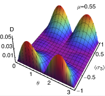
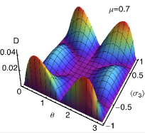
Figure 5: (Color online) Comparison between exact and approximate solution for the mKE estimation of weak hamiltonians. On the left side, the trace distance $D$ between the $H_{exa}$ and the $H_{apx}$ is plotted for a purity of the initial state of $\mu=0.55$. On the right, the trace distance $D$ is displayed for $\mu=0.7$

In order to compare the two Hamiltonians we employ the trace distance, that is:

$$D=\frac{1}{2}\,\mathrm{Tr}\left[{|H_{exa}-H_{apx}|}\right]$$

where $|B|$ is the modulus operator of $B$, i.e. $|B|=\sqrt{B^{\dagger}B}$. We found that this quantity does not depend on the phase $\phi$ of the initial state and shows the same symmetries of the fidelity between the two solutions. In the following we present a brief analysis of the behavior of $D$.

When the initial state $\tau$ is highly mixed the difference between $H_{exa}$ and $H_{apx}$ is small, and reaches a maximal value for $|\langle\sigma_{3}\rangle|\rightarrow 1$ and $\theta=\pi/4$ and $3/4\pi$ (see Fig. 5). This behavior is similar to the one of the fidelity for mixed state, but instead of having a maximal difference for $\theta=\pi/2$, here a minimal difference is found. This is due to different estimates obtained for the components of the Bloch vectors which define the two mKE solutions. In fact, for $\theta=\pi/2$ and $|\langle\sigma_{3}\rangle|\rightarrow 1$, the first two components (here referred to as $\sigma_{1}$ and $\sigma_{2}$) of the Bloch vectors are small but quite different for the exact and the approximate mKE estimates. The last component is anyway equal to one for both the Bloch vectors. The fidelity is able to point this difference out, which however is not affecting the estimation of the Hamiltonians, since the coefficients of the Hamiltonian focus only on the larger component of the Bloch vectors. In turn, the trace distance between the two estimated Hamiltonians do not detect a difference between the approximate and the exact method. The behavior of the distance between the Hamiltonians for $\mu\in[1/2,0.7]$ is analogous, though for increasing $\mu$ another maxima appear, in the same way minima appear for the fidelity.

Let us now address nearly pure initial states: as it is apparent from the comparison of Figs.5 and 6 for increasing $\mu$ we see a transition in the behavior of the trace distance between Hamiltonians: new maxima appear, for $\theta\rightarrow 0,\pi$ and $\langle\sigma_{3}\rangle=0$. and their value increases for $\mu\rightarrow 1$. Overall, the behavior of the trace distance $D$ for nearly pure initial states is analogous to that of the fidelity in the same regime, and all the observations made in that case holds.

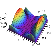
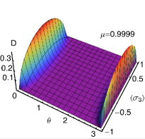
Figure 6: (Color online) Comparison between exact and approximate solution for the mKE estimation of weak hamiltonians. On the left side, the trace distance $D$ between the $H_{exa}$ and the $H_{apx}$ is plotted for a purity of the initial state of $\mu=0.9$. On the right, the trace distance $D$ is displayed for $\mu=0.9999$

V Conclusions

In this paper, we have considered mKE state estimation for qubits when the average of a single observable is available. In particular, a detailed comparison between the approximate and exact solution of the mKE estimation problem has been performed, with the goal of finding the regimes where the approximate solution may be effectively employed. In this case, the advantage is that the approximate solution is given in a closed-form, and it may applied to a larger class of a priori states, including those described by a density operator not having not full rank.

In order to compare the two solutions we have analyzed in details the behavior of fidelity between the two estimated states as a function of the parameters of the initial states and of the outcome of the measurement. Our results show that the most striking difference concerns the purity of the estimated states, with the approximate solution that tends to preserve the purity of the initial state, while the exact one does not, being more sensitive to the information coming from the measurement outcome. Moreover, we find that in terms of fidelity the approximate solution is closer to the initial state than the exact one for the whole range of parameters.

We have also addressed mKE principle as a tools to estimate weak Hamiltonians and compared the performances of the two solutions for this specific task. Employing the trace distance to compare the estimated Hamiltonians, we found results that confirm those obtained analyzing fidelity.

Overall, our analysis shows that approximate solutions to mKE estimation problems may be effectively employed to replace the exact ones unless the initial state is close to an eigenstate of the measured observable. In turns, this provides a rigorous justification for the use of the approximate solution whenever the above condition does not occur.

Appendix A Bloch vector of the approximate solution in Eq. (7)

Upon solving the equation $\hbox{Tr}[\rho(\lambda)\,\sigma_{3}]=\langle\sigma_{3}\rangle$, we obtain an analytic form for the Lagrange multiplier $\lambda$ and, in turn, for the Bloch vector of the approximate solution of Eq. (7)

$$r_{1} =\frac{(\epsilon-1)\sin\theta\cos\phi(\langle\sigma_{3}\rangle(\epsilon-1)\cos\theta+\epsilon+1)\sqrt{1-\frac{(\langle\sigma_{3}\rangle(\epsilon+1)+(\epsilon-1)\cos\theta)^{2}}{(\langle\sigma_{3}\rangle(\epsilon-1)\cos\theta+\epsilon+1)^{2}}}}{(\epsilon-1)^{2}\cos^{2}\theta-(\epsilon+1)^{2}}$$

$$r_{2} =-\frac{(\epsilon-1)\sin\theta\sin\phi(\langle\sigma_{3}\rangle(\epsilon-1)\cos\theta+\epsilon+1)\sqrt{1-\frac{(\langle\sigma_{3}\rangle(\epsilon+1)+(\epsilon-1)\cos\theta)^{2}}{(\langle\sigma_{3}\rangle(\epsilon-1)\cos\theta+\epsilon+1)^{2}}}}{(\epsilon-1)^{2}\cos^{2}\theta-(\epsilon+1)^{2}}$$

$$r_{3} =\langle\sigma_{3}\rangle\,.$$ (12)

References

- (1) G. M. D’Ariano, L. Maccone, M. G. A. Paris, J. Phys. A 34, 93 (2001).
- (2) M. G. A. Paris, J. R̆eháček, Quantum State Estimation, Lect. Notes Phys. 649 (2004).
- (3) Z. Hradil, Phys. Rev. A 55, R1561 (1997).
- (4) Z. Hradil, J. Summhammer, J. Phys. A 33,7607 (2000).
- (5) E. T. Jaynes, Phys. Rev. 106, 620 (1957); ibid. 108, 171 (1957).
- (6) A. Pressé, K. Ghosh, J. Lee, K. A. Dill, Rev. Mod. Phys. 85, 1115 (2013).
- (7) V. Buz̆ek, G. Adam, G. Drobný, G. Adam, Ann. Phys. (N.Y.) 245, 37 (1996); V. Bužek, G. Drobný, G. Adam, R. Derka, and P. Knight, J. Mod. Opt. 44, 2607 (1997).
- (8) M. Ziman, Phys. Rev. A 78, 032118 (2008).
- (9) S. Kullback and R. A. Leibler, Ann. Math. Stat. 22, 79 (1951).
- (10) J. Shore and R. Johnson, IEEE Trans. Inf. Theor. 26 26 (1980).
- (11) T. Georgiou, IEEE Trans. Inf. Theor. 52, 1052 (2006).
- (12) S. Olivares, M. G. A. Paris, Phys. Rev. A 76, 042120 (2007).
- (13) F. Ticozzi and M. Pavon, Quant. Inf. Proc. 9, 551 (2010).
- (14) M. Zorzi, F. Ticozzi, and A. Ferrante, Quantum Inf. Proc. 13, 683 (2014).
- (15) S. Olivares, M. G. A. Paris, Eur. Phys. J. ST 203, 185 (2012).
- (16) M. Zorzi, F. Ticozzi and A. Ferrante, IEEE Trans. Info. Th. 60, 357 (2014).
- (17) H. Umegaki, Kodai Math. Semin. Rep. 14, 59 (1962); G. Linblad, Commun. Math. Phys. 33, 305 (1973).
- (18) F. Hiai, D. Petz, Comm. Math. Phys. 143, 99 (1991).
- (19) M. Hayashi, J. Phys. A 16, 3413 (2001).
- (20) V. Vedral, Rev. Mod. Phys. 74, 197 (2002).
- (21) B. Schumacher and M. Westmoreland, American Mathematical Society Contemporary Mathematics, Series: Quantum Information and Quantum Computation, 305 (American Mathematical Society, Providence, 2002).
- (22) E. G. Galvao, M. B. Plenio, S. Virmani, J. Phys. A 33, 8809 (2000).
- (23) T. Qin, M. Zhao, Y. Zhang, Mod. Phys. Lett. B 22, 313 (2008).
- (24) M. G. Genoni, M. G. A. Paris, K. Banaszek, Phys. Rev. A 78, 060303(R) (2008).
- (25) M. G. Genoni, M. G. A. Paris, Phys. Rev. A 82, 052341 (2010).
- (26) S. L. Braunstein, Phys. Lett. A 219, 169 (1996).
- (27) S. L. Braunstein and C. M. Caves, Phys. Rev. Lett. 72, 3439 (1994).
- (28) See M Bina, A. Mandarino, S. Olivares, M. G. A. Paris, Phys. Rev. A, 89 , 012305 (2014) for a detailed discussion about the properties of states having high fidelity to each other.