A Statistical Model of Current Loops and Magnetic Monopoles

Abstract.

We formulate a natural model of loops and isolated vertices for arbitrary planar graphs, which we call the monopole-dimer model. We show that the partition function of this model can be expressed as a determinant. We then extend the method of Kasteleyn and Temperley-Fisher to calculate the partition function exactly in the case of rectangular grids. This partition function turns out to be a square of a polynomial with positive integer coefficients when the grid lengths are even. Finally, we analyse this formula in the infinite volume limit and show that the local monopole density, free energy and entropy can be expressed in terms of well-known elliptic functions. Our technique is a novel determinantal formula for the partition function of a model of isolated vertices and loops for arbitrary graphs.

1. Introduction

The dimer model on a planar graph $G$ is a statistical mechanical model which idealises the adsorption of diatomic molecules on $G$. The associated combinatorial problem is the weighted enumeration of all dimer covers of $G$, also known as perfect matchings or 1-factors. This problem was solved in a beautiful and explicit way by Kasteleyn [Kas61, Kas63] and by Temperley-Fisher [TF61, Fis61].

The monomer-dimer model on the other hand, which idealises the adsorption of both monoatomic as well as diatomic molecules on $G$, has not had as much success. In this case, one considers the weighted enumeration of all possible matchings of $G$ with separate fugacities for both kinds of molecules. Equivalently, this is the problem of counting all matchings of $G$. There is some indirect evidence that it is not likely to be exactly solvable [Jer87]. It has been rigorously shown that the monomer-dimer model does not exhibit phase transitions [GK71, HL72]. The only solutions so far are obtained by perturbative expansions (see the review in [HL72], for example). The asymptotics of the free energy has been studied by various authors, see [BW66, Ham66, HM70] for instance. There have also been several numerical studies [KRS96, Kon06a, Kon06b] as well as study of monomer correlations in a sea of dimers [FS63]. We note that there has been some success in solving restricted versions of the classical monomer-dimer model exactly, either for finite size or in the limit of infinite size. Such is the case for a single monomer on the boundary [TW03, Wu06], arbitrary monomers on the boundary in the scaling limit [PR08] and a single monomer in the bulk in the thermodynamic limit [BBGJ07, PPR08]. More recently, after the completion of this work, there has appeared a Grassmannian approach to computing the dimer model partition function with fixed locations of monomers exactly [AF14]. On the hexagonal lattice, a lot of work has been done on monomer correlations by Ciucu, see [Ciu10] and references therein.

We note in passing that signed dimer models and signed loop models have gained attention in statistical physics recently, the former in the context of spin liquids [DDR12] and the latter as an approach towards solving the Ising model [KLM13].

In this article, we will consider a signed variant of the monomer-dimer model on any planar graph, which we call the monopole-dimer model. This model will turn out to be a natural generalisation of the well-known dimer model, also defined for any planar graph. The configurations of this model are subgraphs consisting of isolated vertices, doubled edges and oriented loops of even length on the graph such that each vertex is attached to exactly zero or two edges. Each configuration can be thought of as a superposition of two monomer-dimer configurations with the same monomer locations. The reason for the nomenclature will be explained in Section 3, when the weights associated to these configurations are specified. We will prove that the partition function of the monopole-dimer model can be written as a determinant. This property is useful from a computational point of view because one can obtain a lot of information about the model using nothing more than basic linear algebra. This approach has been extremely fruitful in studying many models in statistical physics, such as the Ising model in one-dimension [MW73], the sandpile model [Dha90] and the dimer model for planar graphs [Ken97].

We will use this determinant formula to express the partition function of the monopole-dimer model on the two-dimensional grid as a product. This will turn out to give a natural generalisation of Kasteleyn’s and Temperley-Fisher’s formula for the dimer model on the rectangular grid. It will turn out, for not obvious reasons, that the partition function will be an exact square when the sides of the rectangle are even. This is in contrast to the double-dimer model [Kas61, Fis61], where the partition function is the determinant of an even anti-symmetric matrix, and hence is obviously the square of the corresponding Pfaffian.

We will then derive explicit formulas for the free energy of the monopole-dimer model in terms of known elliptic functions in the infinite size limit and compare it with existing results for the monomer-dimer model, both rigorous and numerical. We will also calculate the entropy and the monopole density. The starting point, namely the determinant formula, is a consequence of a more general model of oriented loops, doubled edges and vertices on a general graph, which we will first explain.

The plan of the paper is as follows. We will first define a new loop-vertex model on arbitrary graphs in Section 2 and show that the partition function of the model can be written as a determinant in Theorem 2.5. We will then define the monopole-dimer model in Section 3 and use results proved in the previous section to show that its partition function can also be written as a determinant in Theorem 3.3. We will then specialise to the two-dimensional grid graph in Section 4 and give an explicit product formula for the partition function in Theorem 4.1. We finally discuss the asymptotic limit of $\mathbb{Z}^{2}$ in Section 5.

The statements of the paper can be verified using the Maple program file Monopole.maple available from the author’s webpage or as an ancillary file from the arXiv source.

2. A Loop-Vertex Model on General Graphs

We begin by defining a model of isolated vertices and loops of even length on arbitrary graphs. The usefulness of the results here is that they are very general, and might be interesting in their own right. At this point, we do not know of any relevant physical situation where this model could be applied. Part of the objective of this section is to make the proof of the determinantal formula for the partition function of the monopole-dimer model simpler. The reader interested in the monopole-dimer model should feel free to skip this section.

Our input data is a simple (not necessarily planar), undirected vertex- and edge-weighted labelled graph $G=[V,E]$ on $n$ vertices and an arbitrary assignment of arrows along each edge, called the orientation $\mathcal{O}$ on $G$. We will denote vertex weights by $x(v)$ for $v\in V$ and edge weights as $a(v,v^{\prime})\equiv a(v^{\prime},v)$ whenever $(v,v^{\prime})\in E$. Any labelled graph comes with a canonical orientation, the one got by directing edges from a lower vertex to a higher one.

Definition 2.1.

A loop-vertex configuration $C$ consists of a subgraph of $G$ of edges which form directed loops of even length including doubled edges (to be thought of as loops of length 2), with the property that every vertex belongs to exactly zero or two edges. Let $\mathcal{L}$ be the set of loop-vertex configurations.

Note that the number of isolated vertices has the same parity as the size of the graph. We first define the signed weight of a loop in $C$. First, the sign of an edge $(v_{1},v_{2})$, denoted $\operatorname{sgn}(v_{1},v_{2})$ is $+1$ if the orientation is from $v_{1}\to v_{2}$ in $\mathcal{O}$ and $-1$ otherwise. Then, given an even oriented loop $\ell=(v_{1},\dots,v_{2n},v_{1})$, the weight of the loop is

(2.1) $$w(\ell)=-\prod_{j=1}^{2n}\operatorname{sgn}(v_{j},v_{j+1})\;a(v_{j},v_{j+1}),$$

with the understanding that $v_{2n+1}=v_{1}$. The reason for the overall minus sign will be clear later. For now, note that the weight of a doubled edge is always $+a(v_{1},v_{2})^{2}$. Lastly, to each isolated vertex $v$, we associate the weight $x(v)$. The weight $w(C)$ of a configuration $C$ is then

(2.2) $$w(C)=\prod_{\ell\text{ a loop}}w(\ell)\prod_{\begin{subarray}{c}v\text{ an }\\ \text{isolated vertex}\end{subarray}}\!\!x(v).$$

Definition 2.2.

The loop-vertex model on a vertex- and edge-weighted graph $G$ is the collection $\mathcal{L}$ of loop-vertex configurations on $G$ with the weight of each configuration given by (2.2).

Figure 1. A non-planar graph $G$ with its natural orientation on the left. A particular loop-vertex configuration is given on the right where the “wrongly” oriented edges are coloured red.

Example 2.3.

For example, the weight of the configuration in Figure 1 is

$$-x(1)\cdot\;a(6,9)^{2}\cdot\;a(2,3)a(3,5)a(5,7)a(7,8)a(4,8)a(2,4)$$

With a slight abuse of terminology, we say that the (signed) partition function of the loop-vertex model on the pair $(G,\mathcal{O})$ is then

(2.3) $$Z_{G,\mathcal{O}}=\sum_{C\in\mathcal{L}}w(C).$$

Whenever the orientation is canonically defined by the labelling on the graph, we will denote the partition function simply as $Z_{G}$.

Definition 2.4.

The signed adjacency matrix $K$ associated to the pair $(G,\mathcal{O})$ is the matrix $K$ indexed by the vertices of $G$ whose entries are

(2.4) $$K(v,v^{\prime})=\begin{cases}x(v)&v^{\prime}=v\\ a(v,v^{\prime})&\text{orientation is from $v$ to $v^{\prime}$ in $\mathcal{O}$}\\ -a(v,v^{\prime})&\text{orientation is from $v^{\prime}$ to $v$ in $\mathcal{O}$}.\end{cases}$$

Theorem 2.5.

The partition function of the loop-vertex model on $(G,\mathcal{O})$ is given by

(2.5) $$Z_{G,\mathcal{O}}=\det K.$$

Proof.

We begin by considering the Leibniz formula for the determinant of $K$. We will consider the permutations in $S_{n}$ according to their cycle decomposition. The first observation is that the sign of a non-trivial odd cycle $c=(c_{1},c_{2},\dots,c_{2l+1},c_{1})$ is the opposite of its reverse $\operatorname{rev}(c)=(c_{1},c_{2l+1},\dots,c_{2},c_{1})$, but the weights are the same. Therefore, such terms cancel out. The only odd cycles which appear are cycles of length one, also known as fixed points.

It is then clear that the terms in the determinant expansion of $K$ are in bijection with loop-vertex configurations of $G$. We now need to show that the signs are the same. Therefore we decompose the permutation $\pi$ into $k$ fixed points and $c$ cycles of lengths $2m_{1},\dots,2m_{c}$. This ensures that $k$ has the same parity as $n$.

A well-known combinatorial result states that if $n$ is odd (resp. even), $\pi$ is odd if and only if the number of cycles is even (resp. odd) in its cycle decomposition. In our case, the number of cycles is $k+c$. A short tabulation shows that the sign of $\pi$ is always the same as $(-1)^{c}$. In other words, the sign of a loop is precisely the product of all the corresponding terms in $K$ plus one extra sign. But this is precisely what we have in (2.1). ∎

Although the loop-vertex model consists of signed weights, the following statement can easily be verified since the signed adjacency matrix is a sum of a diagonal matrix and an antisymmetric matrix.

Corollary 2.6.

The partition function $Z_{G,\mathcal{O}}$ is a positive polynomial in the variables $x(v)$ for $v\in V$ and $a(v,v^{\prime})$ for $(v,v^{\prime})\in E$. In particular, if all the weights are positive reals, $Z_{G,\mathcal{O}}$ is strictly positive.

Example 2.7.

For the loop-vertex model on the complete graph with its canonical orientation (see below (2.3)) with vertex-weights $x$ and edge-weights $a$, the signed adjacency matrix is given by

$$K_{n}=\begin{pmatrix}x&a&a&\cdots&a\\ -a&x&a&\cdots&a\\ \vdots&\ddots&\ddots&\ddots&\vdots\\ -a&\cdots&-a&x&a\\ -a&\cdots&-a&-a&x\end{pmatrix}$$

One can compute the determinant of $K_{n}$ by using elementary row and column operations to convert it to a tridiagonal matrix. It is then easy to show that $Z_{n}$ satisfies the recursion $Z_{n}=2xZ_{n-1}-(x^{2}-a^{2})Z_{n-2}$. It is immediate from the initial conditions $Z_{0}=1$ and $Z_{1}=x$ that

(2.6) $$Z_{n}=\sum_{k=0}^{\lfloor n/2\rfloor}\binom{n}{2k}\;x^{n-2k}\;a^{2k}=\frac{(x+a)^{n}+(x-a)^{n}}{2}.$$

3. The Monopole-Dimer Model on Planar Graphs

We now focus on the model of physical interest, namely the monopole-dimer model. As we shall see, technical reasons force us to restrict our attention to planar graphs. We will first define the model for an arbitrary planar graph and state a theorem about the partition function of the model.

From now on, we will use $G$ to mean both the graph and its planar embedding. As before, $G=[V,E]$ will be a labelled graph with vertex weights $x(v)$ for $v\in V$ and edge weights $a(v,v^{\prime})$ whenever $(v,v^{\prime})\in E$. The configurations of the model are exactly the loop-vertex configurations $\mathcal{L}$ of Definition 2.1. From here on, we will use the term monopole-dimer configurations instead of loop-vertex configurations.

Let $C\in\mathcal{L}$ be a monopole-dimer configuration containing an even loop $\ell$. The weight of the loop $\ell=(v_{1},\dots,v_{2n},v_{1})$ is given by

(3.1) $$w(\ell)=(-1)^{\begin{subarray}{c}\text{number of vertices in $V$}\\ \text{enclosed by $\ell$}\end{subarray}}\prod_{j=1}^{2n}a(v_{j},v_{j+1}),$$

where, as before, $v_{2n+1}\equiv v_{1}$. Notice that the planarity of the graph is used crucially in ensuring that $w(\ell)$ is well-defined. In the usual way, we set the weight of vertex $v$ to be $x(v)$, and the weight $w(C)$ of the entire configuration $C$ as

(3.2) $$w(C)=\prod_{\ell\text{ a loop}}w(\ell)\prod_{v\text{ a vertex}}x(v).$$

Note that the definition of the monopole-dimer model on planar graphs is independent of any orientation, unlike the loop-vertex model.

Definition 3.1.

The monopole-dimer model on $G$ is a model of monopole-dimer configurations $\mathcal{L}$ on $G$ where the weight of each configuration is given by (3.2).

As before, we let the (signed) partition function of the monopole-dimer model on $G$ be

$$Z_{G}=\sum_{\begin{subarray}{c}C\text{ a monopole-dimer}\\ \text{configuration}\end{subarray}}w(C).$$

Remark 3.2.

Configurations of the model are superpositions of two configurations of the monomer-dimer model with identical locations of monomers and thus generalise the so-called double-dimer model [KW11, Ken11]. Since the weight of each double-dimer loop is given a sign which is the parity of the number of monomers enclosed by it, it is reminiscent of the Dirac string representation of the monopole. Dirac had shown by integrating the flux around a curve enclosing the string that the well-definedness of the vector potential led naturally to the quantization of charge [Dir78].

We recall the notion of a Kasteleyn orientation for a planar graph. We will consider the case of bipartite graphs for simplicity; the general case is similar. In this case, Kasteleyn [Kas61] showed that there exists an orientation $\mathcal{O}$ on $G$ such that every basic loop enclosing a face has an odd number of clockwise oriented edges. This is sometimes called the clockwise-odd property. Using this orientation $\mathcal{O}$, Kasteleyn showed that the dimer partition function on $G$ can be written as a Pfaffian of an even antisymmetric matrix, now called the Kasteleyn matrix. Note that the signed adjacency matrix $K$ in (2.4) differs from the Kasteleyn matrix by a diagonal matrix. In what follows, we will refer to the signed adjacency matrix as a (modified) Kasteleyn matrix.

Theorem 3.3.

Let $\mathcal{O}$ be a Kasteleyn orientation on the planar graph $G$ and let $K$ be the modified Kasteleyn matrix defined as (2.4). Then the partition function of the monopole-dimer model on $G$ can be written as

$$Z_{G}=\det K.$$

Moreover, Corollary 2.6 immediately implies that $Z_{G}$ is a positive polynomial in the weights.

Proof.

To prove this, we have to show that the weight of a loop in a planar graph with a Kasteleyn orientation defined by (3.1) is the same as that defined in (2.1). Suppose the loop is of length $2\ell$ and there are $v$ internal vertices, $e$ internal edges and $f$ faces. Suppose the Kasteleyn orientation is such that there are $o_{j}$ clockwise edges in face $j$, where each $o_{j}$ is odd. The total number of clockwise edges on the loop is therefore $\sum_{j=1}^{f}o_{j}-e$ since each internal edge contributes twice to the count, once clockwise and once counter-clockwise. The Euler characteristic $v-e+f$ is 1 on the plane since we exclude the unbounded face. Since the parity of $\sum_{j=1}^{f}o_{j}-e$ is the same as that of $f-e$, which equals $v-1$, we have shown that the total number of clockwise edges on the loop is odd if and only if $v$ is even. This shows that the weights in (3.1) and (2.1) coincide. ∎

Example 3.4.

Consider the cycle graph $C_{n}$ where the vertices are labelled in cyclic order with the canonical orientation with weights $a$ to each edge and $x$ to each vertex. The modified Kasteleyn matrix $K_{n}$ is then

$$K_{n}=\begin{pmatrix}x&a&0&\cdots&a\\ -a&x&a&\cdots&0\\ &\ddots&\ddots&\ddots&\\ 0&\cdots&-a&x&a\\ -a&0&\cdots&-a&x\end{pmatrix}.$$

One can then show with a little bit of work that the partition function $Z_{n}$ satisfies

$$Z_{n}=\det K_{n}=\begin{cases}xa^{n}F_{n}\left(\frac{x}{a}\right)+2a^{n+1}F_{n-1}\left(\frac{x}{a}\right),&\text{if $n$ is odd},\\ xa^{n-1}F_{n}\left(\frac{x}{a}\right)+2a^{n}F_{n-1}\left(\frac{x}{a}\right)+2a^{n},&\text{if $n$ is even},\end{cases}$$

where $F_{n}(x)$ is the $n$’th Fibonacci polynomial defined by the recurrence $F_{n}(x)=xF_{n-1}(x)+F_{n-2}(x)$ with initial conditions $F_{0}(x)=0$ and $F_{1}(x)=1$. Using standard properties of the Fibonacci polynomials, we can rewrite

$$Z_{n}=\begin{cases}\displaystyle a^{n}\;L_{n}\left(\frac{x}{a}\right)&\text{if $n$ is odd},\\ \\ \displaystyle a^{n}\;\left(L_{n/2}\left(\frac{x}{a}\right)\right)^{2}&\text{if $n\equiv 0\;(\bmod\;4)$ },\\ \\ \displaystyle a^{n-2}\;(x^{2}+4a^{2})\;\left(F_{n/2}\left(\frac{x}{a}\right)\right)^{2}&\text{if $n\equiv 2\;(\bmod\;4)$ }.\end{cases}$$

where the Lucas polynomials $L_{n}(x)$ satisfy the same recurrence as the Fibonacci polynomials but with different initial conditions, $L_{0}(x)=2$ and $L_{1}(x)=x$.

Remark 3.5.

Note that when $n$ is divisible by 4, $\sqrt{Z_{n}}$ is a positive polynomial and can be considered as the partition function of a model of monomers and dimers. This phenomenon will recur in Section 4.

Corollary 3.6 (Kasteleyn [Kas61]).

In the absence of vertex weights, i.e. $x(v)=0\;\forall\;v\in V$, the monopole-dimer model is exactly the double-dimer model (see Remark 3.2) and consequently, $Z_{G}=|\operatorname{Pf}K|^{2}$.

We will now explore some consequences of the determinant formula for the monopole-dimer model. Unlike for the usual dimer model, one cannot calculate probabilities of events for the monopole-dimer model since the measure on configurations here is not positive. However, one can consider expectations of observables in this signed measure.

Definition 3.7.

The joint correlation of a subconfiguration of monopoles $v_{1},\dots,v_{j}$ and loops $\ell_{1},\dots,\ell_{k}$ in the graph $G$ is

$$\langle v_{1},\dots,v_{j};\ell_{1},\dots,\ell_{k}\rangle=\prod_{r=1}^{j}x(v_{r})\prod_{s=1}^{k}w(\ell_{s})\;\frac{\widehat{Z}_{G^{\prime}}}{Z_{G}}$$

where $G^{\prime}$ is the subgraph of $G$ with the vertices $v_{1},\dots,v_{j}$ and those in loops $\ell_{1},\dots,\ell_{k}$ removed; and $\widehat{Z}_{G^{\prime}}$ is the partition function of the monopole-dimer model in $G^{\prime}$ with the caveat that the sign of loops in $G^{\prime}$ given by (3.1) be taken by considering vertices in all of $G$

To give a formula for joint correlations, we recall the complementary minor identity of Jacobi. For a $k\times k$ nonsingular matrix $A$, $1\leq i\leq k$, sequences $[p]=(p_{1},\dots,p_{i}),[q]=(q_{1},\dots,q_{i})$ where $1\leq p_{1}<\cdots<p_{i}\leq k$ and $1\leq q_{1}<\cdots<q_{i}\leq k$, let $A^{[p]}_{[q]}$ be the $i\times i$ submatrix of $A$ consisting of rows $p_{j}$ and columns $q_{j}$. Also, let $[\bar{p}]$ (resp. $[\bar{q}]$) be the complementary sets $\{1,\dots,k\}\setminus[p]$ (resp. $\{1,\dots,k\}\setminus[q]$). Recall that the determinant of such a submatrix is called a minor, and when $[p]=[q]$, both the submatrix and its minor are qualified by the adjective principal.

Theorem 3.8 (Jacobi, see $\S 14.16$ of [GR00]).

$$\det\left((A^{-1})^{[\bar{q}]}_{[\bar{p}]}\right)=\frac{(-1)^{p_{1}+q_{1}+\cdots+p_{i}+q_{i}}}{\det A}\det A^{[p]}_{[q]}.$$

Remark 3.9.

In the case of an unsigned combinatorial model on a graph (i.e. with nonnegative weights) whose partition function can be written as a determinant, Theorem 3.8 implies that probabilities of local events can be computed in terms of principal minors of the inverse. This fact has been used with great success for the dimer model [Ken97].

Lemma 3.10.

Let $[\bar{p}]$ be the set of vertices of monopoles $v_{1},\dots,v_{j}$ and of loops $\ell_{1},\dots,\ell_{k}$. Then the joint correlation is given by

$$\langle v_{1},\dots,v_{j};\ell_{1},\dots,\ell_{k}\rangle=\prod_{r=1}^{j}x(v_{r})\prod_{s=1}^{k}w(\ell_{s})\;\det\left((K^{-1})^{[\bar{p}]}_{[\bar{p}]}\right).$$

Furthermore, it is positive if the subconfiguration has positive weight.

Proof.

The sum over all configurations with these prescribed monopoles and loops is given by the appropriate principal minor of the modified Kasteleyn matrix, $K$. By Theorem 3.8, this is exactly the complementary minor of the inverse, which exists because of Corollary 2.6. The minor is the determinant of a matrix which is the sum of an antisymmetric matrix and a diagonal matrix and is positive, again using Corollary 2.6. Thus, the only way for the joint correlation to be negative is if the subconfiguration itself has negative weight. ∎

We will use Lemma 3.10 in the following to compute monopole correlations. The joint correlation of the monopole-loop configuration on the right side of Figure 2 in a large $m\times n$ square is the simplest example of one which is negative.

4. The Monopole-Dimer model on the Rectangular Grid

We will now calculate the partition function for the monopole-dimer model in Section 3 on the rectangular grid graph, thereby generalising the famous product formula of Temperley-Fisher [Fis61] and Kasteleyn [Kas61].

Consider the $m\times n$ grid $Q_{m,n}=\{(i,j)\;|\;1\leq i\leq m,1\leq j\leq n\}$ with horizontal edge-weights $a$, vertical edge-weights $b$ and vertex-weights $z$. For the sake of completeness, we recall the Kasteleyn orientation $\mathcal{O}$ prescribed independently by Fisher [Fis61] and Kasteleyn [Kas61]. The arrow always points in the direction $(i,j)\to(i,j+1)$, i.e., towards the positive $x$-axis. In the $y$-direction, the arrow points from $(i,j)\to(i,j+1)$ (i.e. towards the positive $y$-axis) whenever $i$ is odd and in the reverse direction when $i$ is even. This orientation can be easily seen to be induced by a “snake-like” labelling, as seen in Figure 2.

Define the function

$$Y_{m}(b;z)=\prod_{j=1}^{\lfloor m/2\rfloor}\left(z^{2}+4b^{2}\cos^{2}\frac{j\pi}{m+1}\right).$$

Theorem 4.1.

The partition function of the monopole-dimer model on $Q_{m,n}$ is given by

(4.1) $$\begin{split}Z_{{m,n}}=&\prod_{j=1}^{\lfloor m/2\rfloor}\prod_{k=1}^{\lfloor n/2\rfloor}\left(z^{2}+4b^{2}\cos^{2}\frac{j\pi}{m+1}+4a^{2}\cos^{2}\frac{k\pi}{n+1}\right)^{2}\\ &\times\begin{cases}1&\text{if $m$ and $n$ are even},\\ Y_{m}(b;z)&\text{if $m$ is even and $n$ is odd},\\ Y_{n}(a;z)&\text{if $m$ is odd and $n$ is even},\\ zY_{m}(b;z)Y_{n}(a;z)&\text{if $m$ and $n$ are odd}.\end{cases}\end{split}$$

Proof.

The matrix $K_{m,n}$ is exactly the regular Kasteleyn matrix added to $z$ times the identity matrix of size $mn$. Therefore, the inversion technique described in either of these papers works identically when $m$ or $n$ are even. The case when both $m$ and $n$ are odd is a special case, which has to be worked out separately. Both cases can be analysed simultaneously.

We use Fisher’s labelling [Fis61]. The modified Kasteleyn matrix can be written in $m\times m$ tridiagonal block form

$$K=\begin{pmatrix}X&Y&0&0&\cdots&0\\ -Y&X&Y&0&\cdots&0\\ 0&-Y&X&Y&\cdots&0\\ \vdots&\ddots&\ddots&\ddots&\ddots&\vdots\\ 0&\cdots&0&-Y&X&Y\\ 0&0&\cdots&0&-Y&X\end{pmatrix},$$

where each of the blocks is an $n\times n$ matrix with

$$X=\begin{pmatrix}z&a&0&0&\cdots&0\\ -a&z&a&0&\cdots&0\\ 0&-a&z&a&\cdots&0\\ \vdots&\ddots&\ddots&\ddots&\ddots&\vdots\\ 0&\cdots&0&-a&z&a\\ 0&0&\cdots&0&-a&z\end{pmatrix},\quad\text{ and }Y=\begin{pmatrix}0&\cdots&0&0&b\\ 0&\cdots&0&b&0\\ \vdots&\mathinner{\mkern 1.0mu\raise 1.0pt\vbox{\kern 7.0pt\hbox{.}}\mkern 2.0mu\raise 4.0pt\hbox{.}\mkern 2.0mu\raise 7.0pt\hbox{.}\mkern 1.0mu}&\mathinner{\mkern 1.0mu\raise 1.0pt\vbox{\kern 7.0pt\hbox{.}}\mkern 2.0mu\raise 4.0pt\hbox{.}\mkern 2.0mu\raise 7.0pt\hbox{.}\mkern 1.0mu}&\mathinner{\mkern 1.0mu\raise 1.0pt\vbox{\kern 7.0pt\hbox{.}}\mkern 2.0mu\raise 4.0pt\hbox{.}\mkern 2.0mu\raise 7.0pt\hbox{.}\mkern 1.0mu}&\vdots\\ 0&b&0&\cdots&0\\ b&0&0&\cdots&0\end{pmatrix}.$$

Fisher showed [Fis61] that the matrix $K$ can be simplified considerably by the unitary transformation $U=u_{m}\otimes u_{n}$ where $u_{s}$ is an $s\times s$ matrix with entries

(4.2) $$(u_{s})_{p,q}=\sqrt{\frac{2}{s+1}}i^{p}\sin\frac{\pi pq}{s+1},$$

where $i=\sqrt{-1}$. $u_{s}^{-1}$ also has an equally simple formula

(4.3) $$(u_{s})^{-1}_{p,q}=\sqrt{\frac{2}{s+1}}(-i)^{q}\sin\frac{\pi pq}{s+1}.$$

One can show that $U^{-1}\,K\,U$ can be written as a block diagonal matrix of $\chi_{s}$’s for $s=1,\dots,m$, where

(4.4) $$\chi_{s}=\begin{pmatrix}\scriptstyle z+2ia\cos\frac{\pi}{n+1}&\scriptstyle 0&\dots&\scriptstyle 0&\scriptstyle(-1)^{n-1}2i^{n}b\cos\frac{\pi s}{m+1}\\ \scriptstyle 0&\scriptstyle z+2ia\cos\frac{2\pi}{n+1}&&\scriptstyle(-1)^{n-2}2i^{n}b\cos\frac{\pi s}{m+1}&\scriptstyle 0\\ \vspace{-0.2cm}\vdots&&\ddots\mathinner{\mkern 1.0mu\raise 1.0pt\vbox{\kern 7.0pt\hbox{.}}\mkern 2.0mu\raise 4.0pt\hbox{.}\mkern 2.0mu\raise 7.0pt\hbox{.}\mkern 1.0mu}&&\vdots\\ \vdots&&\mathinner{\mkern 1.0mu\raise 1.0pt\vbox{\kern 7.0pt\hbox{.}}\mkern 2.0mu\raise 4.0pt\hbox{.}\mkern 2.0mu\raise 7.0pt\hbox{.}\mkern 1.0mu}\ddots&&\vdots\\ \scriptstyle 0&\scriptstyle(-1)^{1}2i^{n}b\cos\frac{\pi s}{m+1}&&\scriptstyle z+2ia\cos\frac{(n-1)\pi}{n+1}&\scriptstyle 0\\ \scriptstyle(-1)^{0}2i^{n}b\cos\frac{\pi s}{m+1}&\scriptstyle 0&\dots&\scriptstyle 0&\scriptstyle z+2ia\cos\frac{n\pi}{n+1}\end{pmatrix}$$

Let us now look at each of the cases. When $n$ is even, the determinant of $\chi_{s}$ is easily expressed as a product of $2\times 2$ determinants,

$$\det\chi_{s} =\prod_{p=1}^{\frac{n}{2}}\begin{vmatrix}\displaystyle z+2ia\cos\frac{p\pi}{n+1}&(-1)^{n-p}2i^{n}b\cos\frac{s\pi}{m+1}\\ \\ \displaystyle(-1)^{p-1}2i^{n}b\cos\frac{s\pi}{m+1}&z+2ia\cos\frac{(n+1-p)\pi}{n+1}\end{vmatrix}$$

$$=\prod_{p=1}^{\frac{n}{2}}\left(z^{2}+4b^{2}\cos^{2}\frac{s\pi}{m+1}+4a^{2}\cos^{2}\frac{p\pi}{n+1}\right)=\det\chi_{m+1-s}.$$

When $m$ is also even, we get after multiplying over all $s$, precisely the formula in the first case (4.1). When $m$ is odd, we get an additional factor $|\chi_{(m+1)/2}|$, which is easy to compute because it is a diagonal matrix. The factor we get is

$$\det\chi_{(m+1)/2} =\prod_{p=1}^{n}\left(z+2ia\cos\frac{p\pi}{n+1}\right)$$

$$=\prod_{p=1}^{\frac{n}{2}}\left(z^{2}+4a^{2}\cos^{2}\frac{p\pi}{n+1}\right)=Y_{n}(a;z).$$

This also matches with (4.1). When $n$ is odd and $m$ is even, we have the additional factor contributing to each $|\chi_{s}|$ from the central term,

$$z+2ib\cos\frac{\pi s}{m+1}.$$

Multiplying this factor for all $s$ gives us $Y_{m}(b;z)$ as needed. The last case when both $m$ and $n$ are odd gives us both the factors above and an additional term corresponding to the central entry of the central block matrix, which can be seen to be $z$. ∎

Figure 2. The graph $Q_{3,3}$ of Example 4.2 with its natural orientation on the left and a particular monopole-dimer configuration on the right.

Example 4.2.

Consider the first nontrivial case: $m=n=3$. Figure 2 shows $Q_{3,3}$ with a Kasteleyn orientation and one of two configurations which contribute with a weight $-za^{4}b^{4}$. The modified Kasteleyn matrix is given by

$$K_{{3,3}}=\left(\begin{array}[]{ccccccccc}z&a&0&0&0&b&0&0&0\\ -a&z&a&0&b&0&0&0&0\\ 0&-a&z&b&0&0&0&0&0\\ 0&0&-b&z&a&0&0&0&b\\ 0&-b&0&-a&z&a&0&b&0\\ -b&0&0&0&-a&z&b&0&0\\ 0&0&0&0&0&-b&z&a&0\\ 0&0&0&0&-b&0&-a&z&a\\ 0&0&0&-b&0&0&0&-a&z\\ \end{array}\right)$$

The partition function is given by

$$Z_{{3,3}}=z\left(2a^{2}+z^{2}\right)\left(2b^{2}+z^{2}\right)\left(2a^{2}+2b^{2}+z^{2}\right)^{2},$$

in agreement with (4.1).

Remark 4.3.

The fact that the partition function $Z_{m,n}$ is an exact square of a positive polynomial when $m$ and $n$ are even is nontrivial since $K_{m,n}$ is not antisymmetric.

We will now use Theorem 3.8 to calculate joint correlations in the monopole-dimer model on the grid graph. We focus on the case when $m,n$ are even for simplicity. To do so, we will first need to calculate the matrix entries for the inverse of the modified Kasteleyn matrix. We will now calculate this in full generality. Since we have used the snake-like Kasteleyn orientation explained at the beginning of this Section, the relationship between the entries of the matrix and coordinates on the grid depends on the parity of the abscissa. To simplify notation, we define the functions

$$\phi_{g,h}(c,d;e,f)=\frac{4i^{c+d}(-i)^{e+f}}{(m+1)(n+1)} \sin\frac{\pi cg}{m+1}\sin\frac{\pi eg}{m+1}\sin\frac{\pi dh}{n+1}\sin\frac{\pi fh}{n+1}$$

$$\times\left(\frac{z-2ia\cos\frac{\pi h}{n+1}+(-1)^{f+h}2i^{n}b\cos\frac{\pi g}{m+1}}{z^{2}+4a^{2}\cos^{2}\frac{\pi h}{n+1}+4b^{2}\cos^{2}\frac{\pi g}{m+1}}\right),$$

$$\psi_{g,h}(c,d;e,f)=\frac{4i^{c+d}(-i)^{e+f}}{(m+1)(n+1)} \sin\frac{\pi cg}{m+1}\sin\frac{\pi eg}{m+1}\sin\frac{\pi dh}{n+1}\sin\frac{\pi fh}{n+1}$$

$$\times\left(\frac{z-2ia\cos\frac{\pi h}{n+1}+(-1)^{f+h-1}2i^{n}b\cos\frac{\pi g}{m+1}}{z^{2}+4a^{2}\cos^{2}\frac{\pi h}{n+1}+4b^{2}\cos^{2}\frac{\pi g}{m+1}}\right),$$

for fixed $m,n$ and weights $a,b,z$. The only difference between the two functions is the power of $-1$ in the last term of the numerator inside the parenthesis.

Lemma 4.4.

If $n$ is even, the entries of the inverse matrix are given by

$$\left(K_{m,n}^{-1}\right)_{(c,d),(e,f)}=\sum_{(g,h)\in Q_{m,n}}\begin{cases}\phi_{g,h}(c,d;e,f)&\text{if both $c$ and $e$ are odd,}\\ \phi_{g,h}(c,n+1-d;e,f)&\text{if $c$ is even and $e$ is odd,}\\ \phi_{g,h}(c,d;e,n+1-f)&\text{if $c$ is odd and $e$ is even,}\\ \phi_{g,h}(c,n+1-d;e,n+1-f)&\text{if both $c$ and $e$ are even,}\\ \end{cases}$$

and if $n$ is odd, the entries are given by

$$\left(K_{m,n}^{-1}\right)_{(c,d),(e,f)}=\sum_{(g,h)\in Q_{m,n}}\begin{cases}\psi_{g,h}(c,d;e,f)&\text{if both $c$ and $e$ are odd,}\\ \psi_{g,h}(c,n+1-d;e,f)&\text{if $c$ is even and $e$ is odd,}\\ \psi_{g,h}(c,d;e,n+1-f)&\text{if $c$ is odd and $e$ is even,}\\ \psi_{g,h}(c,n+1-d;e,n+1-f)&\text{if both $c$ and $e$ are even.}\\ \end{cases}$$

Proof.

Since $U^{-1}\,K_{m,n}\,U=\text{Diag}(\chi_{1},\dots,\chi_{m})$, where $\chi_{s}$ is given in (4.4) and $U=u_{m}\otimes u_{n}$, $U^{-1}$ are given explicitly in (4.2),(4.3), one starts by inverting $\chi_{s}$ and obtains $K_{m,n}^{-1}$ as $U^{-1}\,\text{Diag}(\chi_{1}^{-1},\dots,\chi_{m}^{-1})\,U$ by a somewhat lengthy but straightforward calculation.

The parities of $c$ and $e$ enter in the calculation simply because in the Kasteleyn orientation, the coordinates $d,f$ increase from left to right when $c,e$ are odd and from right to left, when $c,e$ are even; see Figure 2 for example. ∎

Corollary 4.5.

The one-point monopole correlation (informally the density) at $(c,d)$ in the $m\times n$ grid is given by

$$\frac{4z^{2}}{(m+1)(n+1)}\sum_{(g,h)\in Q_{m,n}}\!\!\frac{\sin^{2}\frac{\pi cg}{m+1}\sin^{2}\frac{\pi dh}{n+1}}{z^{2}+4a^{2}\cos^{2}\frac{\pi h}{n+1}+4b^{2}\cos^{2}\frac{\pi g}{m+1}}.$$

Proof.

As per the definition of the correlation and Theorem 3.8, the one-point monopole correlation at $(c,d)$ is given by $z\;K^{-1}_{(c,d),(c,d)}$. We use Lemma 4.4 and use the symmetry of $\phi_{g,h}(c,d;c,d)$ and $\psi_{g,h}(c,d;c,d)$ under the transformations $g\mapsto m+1-g$ and $h\mapsto n+1-h$ to obtain the result. ∎

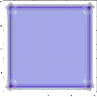
Figure 3. A contour plot of exact monopole densities as a function of location in a $20\times 20$ grid for $a=b=z=1$. Note the uniformity of the density in the interior of the system.

As expected, the prefactor of $z^{2}$ ensures that there is one additional monopole when either $m$ or $n$ is even. See, for example, Figure 3 for the density plot when $m=n=20$. One can also compute joint correlations of monopoles. For instance, the two-point correlation of monopoles at positions $(c,d)$ and $(e,f)$ far apart is given by

$$\det\left(\begin{matrix}K^{-1}_{(c,d),(c,d)}&K^{-1}_{(c,d),(e,f)}\\ K^{-1}_{(e,f),(c,d)}&K^{-1}_{(e,f),(e,f)}\end{matrix}\right).$$

5. Discussion on Asymptotic Behaviour

We will now focus on asymptotic results for the monopole-dimer model on the grid graph. The results in this section will be less formal and will focus more on obtaining rough estimates for the equivalent of quantities in standard thermodynamics, such as the free energy, density and the entropy. Part of the reason for the informality of this section is that we are manipulating $Z_{m,n}$ as if it were the standard partition function in statistical physics. This is not strictly allowed because our partition functions are signed sums. However, as we shall see, we can justify this a posteriori by showing that the results are sensible.

Just as at the end of the previous section, $m,n$ are assumed to be even for simplicity. The free energy is then given by

$$F(a,b,z)=\lim_{m,n\to\infty}\frac{1}{mn}\ln Z_{{m,n}}.$$

Using (4.1), one can treat the right hand side as a Riemann sum, which tends to the limit

$$F(a,b,z)=\frac{2}{\pi^{2}}\int_{0}^{\pi/2}\text{d}\theta \int_{0}^{\pi/2}\text{d}\phi\;\ln\left(z^{2}+4a^{2}\cos^{2}\theta+4b^{2}\cos^{2}\phi\right).$$

Following standard thermodynamic relations, the density of $a$-type of dimers (and similarly, the $b$-type) and that of monopoles is given, after differentiating under the integral sign, by

(5.1) $$\rho_{a} =a\frac{\partial}{\partial a}F(a,b,z)=\frac{2}{\pi^{2}}\int_{0}^{\pi/2}\text{d}\theta \int_{0}^{\pi/2}\text{d}\phi\;\frac{8a^{2}\cos^{2}\theta}{z^{2}+4a^{2}\cos^{2}\theta+4b^{2}\cos^{2}\phi},$$

(5.2) $$\rho_{z} =z\frac{\partial}{\partial z}F(a,b,z)=\frac{2}{\pi^{2}}\int_{0}^{\pi/2}\text{d}\theta \int_{0}^{\pi/2}\text{d}\phi\;\frac{2z^{2}}{z^{2}+4a^{2}\cos^{2}\theta+4b^{2}\cos^{2}\phi}.$$

It is easy to see that $\rho_{a}+\rho_{b}+\rho_{z}=1.$ This is to be expected since each vertex either contains a monopole or is part of a loop adjacent to either an $a$ or a $b$ dimer.

One of the integrals in each case is easily done. Surprisingly, $\rho_{a}$ is easier to evaluate than $\rho_{z}$ even though the final formula will turn out to be simpler for the latter.

$$\rho_{a}=\frac{2}{\pi}\int_{0}^{\pi/2}\text{d}\theta\frac{4a^{2}\cos^{2}\theta}{\sqrt{(z^{2}+4a^{2}\cos^{2}\theta)(z^{2}+4b^{2}+4a^{2}\cos^{2}\theta)}}$$

After the change of variables $t=(2a\cos\theta)^{-1}$, we obtain

$$\rho_{a}=\frac{1}{\pi ayz}\int_{1/2a}^{\infty}\frac{\text{d}t}{t\sqrt{(t^{2}-\frac{1}{4a^{2}})(t^{2}+\frac{1}{z^{2}})(t^{2}+\frac{1}{y^{2}})}},$$

where $y^{2}=z^{2}+4b^{2}$. Using a known formula for elliptic integrals [GR00][(3.137), Formula 8] and an amazing transformation [AS64][Formula 17.7.14], it turns out that $\rho_{a}$ can be concisely expressed in terms of a single known special function, the Heuman Lambda function $\Lambda_{0}(\theta,k)$, defined in [AS64, Formula 17.4.39], as

(5.3) $$\rho_{a}=1-\Lambda_{0}(\theta_{a},k),$$

where all the complexity has been absorbed in the parameters

(5.4) $$\theta_{a}=\tan^{-1}\left(\sqrt{\frac{4b^{2}+z^{2}}{4a^{2}}}\right),\;\text{ and }k=\frac{4ab}{\sqrt{(4a^{2}+z^{2})(4b^{2}+z^{2})}},$$

where $k$ is the standard notation for the elliptic modulus. We remark that the Heuman Lambda function is an elliptic function related to the Jacobi Zeta function and has come up in various physical problems. It turns out that the monopole density can be written, using a miraculous addition formula for $\Lambda$ [BF71, Formula 153.01] as

(5.5) $$\rho_{z}=\frac{K(k)\;k\;z^{2}}{2\,\pi\,a\,b},$$

where $K(k)$ is the complete elliptic integral of the first kind. Now that we have expressions for $\rho_{a}$ and $\rho_{z}$, we would like to obtain a simple expression for the free energy $F(a,b,z)$ by integrating $\frac{\rho_{z}}{z}$.

Starting with the series expansion for $K(k)$ in [AS64, Formula 17.3.11], we get

(5.6) $$\rho_{z}=\frac{z^{2}}{\sqrt{(4a^{2}+z^{2})(4b^{2}+z^{2})}}\sum_{j=0}^{\infty}\left(\frac{(2j-1)!!}{2^{j}j!}\right)^{2}\left(\frac{16a^{2}b^{2}}{(4a^{2}+z^{2})(4b^{2}+z^{2})}\right)^{j}.$$

We now integrate $\frac{\rho_{z}}{z}$ term by term assuming $a>b$ and obtain, using a standard computer algebra package, an infinite sum involving $2F1-$hypergeometric functions,

(5.7) $$\begin{split}F(a,b,z)=\sqrt{\frac{4b^{2}+z^{2}}{a^{2}-b^{2}}}\;&\sum_{j=0}^{\infty}\;\frac{1}{2j-1}\;\binom{2j}{j}^{2}\\ &\times\left(\frac{a^{2}b^{2}}{(a^{2}-b^{2})(4b^{2}+z^{2})}\right)^{j}{}_{2}F_{1}{\left[\genfrac{.}{.}{0.0pt}{}{\frac{1}{2}-j\mskip 8.0mu\frac{1}{2}+j}{\frac{3}{2}-j};\frac{4b^{2}+z^{2}}{4b^{2}-4a^{2}}\right]}\end{split}$$

Since the integrands are symmetric in $a$ and $b$, we can obtain the free energy when $b>a$ by interchanging $a$ and $b$ in (5.7). We handle the $a=b$ case separately. In particular, we set them equal to 1 without loss of generality. In that case, each integral in (5.6) is easier because of the absence of square roots and it turns out that we can write $F(1,1,z)$ again using a computer algebra package as

(5.8) $$F(1,1,z)=\frac{1}{2}\ln(4+z^{2})-\frac{1}{(4+z^{2})^{2}}\;{}_{4}F_{3}{\left[\genfrac{.}{.}{0.0pt}{}{1\mskip 8.0mu1\mskip 8.0mu\frac{3}{2}\mskip 8.0mu\frac{3}{2}}{2\mskip 8.0mu2\mskip 8.0mu2};\frac{16}{(4+z^{2})^{2}}\right]}$$

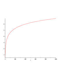
Figure 4. A plot of $F(1,1,z)$ for $z$ varying between 0 and 1000.

As expected from general statistical physical considerations, $F(1,1,z)$ grows monotonically in $z$ and is concave [Ham66] as seen in Figure 4. In accordance with the intuition developed for the monomer-dimer model [GK71, HL72], $F(1,1,z)$ is smooth and there are no phase transitions. One can verify that $F(1,1,0)=2G/\pi$, where $G$ is Catalan’s constant. This is expected since this model reduces, when $z=0$, to the double-dimer model, which is the square of the dimer model [Kas61, Fis61].

Since configurations of the monopole-dimer model are superpositions of two dimer model configurations with fixed monopole locations, and since $Z_{m,n}$ turns out to be a perfect square, we can compare $\sqrt{Z_{m,n}}$ with existing literature on the monomer-dimer model. $F(1,1,z)/2$ compares favourably with rigorous bounds for the free energy of the classical monomer-dimer model in the literature, although it is not very close to numerical data; see Figure 5. Note that the plot here is as a function of dimer density $\rho=\rho_{a}+\rho_{b}$, not $z$. The transformation is a classic exercise in demonstrating equivalence of ensembles. See [Kon06b, Appendix A] for example.

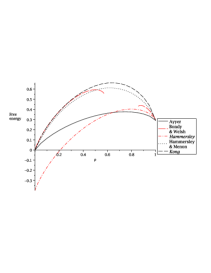
Figure 5. Comparison of $F(1,1,z)/2$ with bounds obtained in [BW66, Ham66, HM70] and recent numerics in [Kon06b].

One can also calculate the entropy using standard thermodynamic relations,

$$S(a,b,z) =F(a,b,z)-z\ln z\frac{\partial}{\partial z}F(a,b,z)$$

$$=F(a,b,z)-\rho_{z}\ln z.$$

In the special case of equal dimer weights, this leads to

$$S(1,1,z)=F(1,1,z)-\frac{2z^{2}\ln z}{\pi(4+z^{2})}K\left(\frac{4}{4+z^{2}}\right).$$

Using (5.8), one can show that the entropy is maximum when $z=1$, at which point the monopole density using (5.5) is

$$\rho_{z}=\frac{2}{5\pi}K\left(\frac{4}{5}\right)\approx 0.25404.$$

This compares very well with the exact result for the $20\times 20$ grid in Figure 3.

Many qualitative properties of the monopole-dimer model on grids are similar to those of the classical monomer-dimer model, which is of much interest to scientists in various fields. The exact formulas for grids presented here might be used to gain further insight about the monomer-dimer model. The determinantal character of the partition function for the loop-vertex model on general graphs and the monopole-dimer model on planar graphs might also prove useful in other contexts.

References

- [AF14] Nicolas Allegra and Jean-Yves Fortin. Grassmannian representation of the two-dimensional monomer-dimer model. Phys. Rev. E, 89:062107, Jun 2014.
- [AS64] Milton Abramowitz and Irene A. Stegun. Handbook of mathematical functions with formulas, graphs, and mathematical tables, volume 55 of National Bureau of Standards Applied Mathematics Series. For sale by the Superintendent of Documents, U.S. Government Printing Office, Washington, D.C., 1964.
- [BBGJ07] J. Bouttier, M. Bowick, E. Guitter, and M. Jeng. Vacancy localization in the square dimer model. Physical Review E, 76(4):041140, 2007.
- [BF71] Paul F. Byrd and Morris D. Friedman. Handbook of elliptic integrals for engineers and scientists. Die Grundlehren der mathematischen Wissenschaften, Band 67. Springer-Verlag, New York, 1971. Second edition, revised.
- [BW66] J. A. Bondy and D. J. A. Welsh. A note on the monomer dimer problem. In Mathematical Proceedings of the Cambridge Philosophical Society, volume 62, pages 503–505. Cambridge Univ Press, 1966.
- [Ciu10] Mihai Ciucu. The emergence of the electrostatic field as a Feynman sum in random tilings with holes. Trans. Amer. Math. Soc., 362(9):4921–4954, 2010.
- [DDR12] Kedar Damle, Deepak Dhar, and Kabir Ramola. Resonating valence bond wave functions and classical interacting dimer models. Phys. Rev. Lett., 108:247216, Jun 2012.
- [Dha90] D. Dhar. Self-organized critical state of sandpile automaton models. Physical Review Letters, 64(14):1613–1616, 1990.
- [Dir78] P. A. M. Dirac. The monopole concept. International Journal of Theoretical Physics, 17(4):235–247, 1978.
- [Fis61] Michael E Fisher. Statistical mechanics of dimers on a plane lattice. Physical Review, 124(6):1664, 1961.
- [FS63] Michael E Fisher and John Stephenson. Statistical mechanics of dimers on a plane lattice. ii. dimer correlations and monomers. Physical Review, 132(4):1411, 1963.
- [GK71] C. Gruber and H. Kunz. General properties of polymer systems. Communications in Mathematical Physics, 22(2):133–161, 1971.
- [GR00] I. S. Gradshteyn and I. M. Ryzhik. Table of integrals, series, and products. Academic Press, Inc., San Diego, CA, sixth edition, 2000. Translated from the Russian, Translation edited and with a preface by Alan Jeffrey and Daniel Zwillinger.
- [Ham66] J. M. Hammersley. Existence theorems and Monte Carlo methods for the monomer-dimer problem. In Research Papers in Statistics (Festschrift J. Neyman), pages 125–146. John Wiley, London, 1966.
- [HL72] Ole J. Heilmann and Elliott H. Lieb. Theory of monomer-dimer systems. Communications in Mathematical Physics, 25(3):190–232, 1972.
- [HM70] J. M. Hammersley and V. V. Menon. A lower bound for the monomer-dimer problem. IMA Journal of Applied Mathematics, 6(4):341–364, 1970.
- [Jer87] Mark Jerrum. Two-dimensional monomer-dimer systems are computationally intractable. Journal of Statistical Physics, 48(1):121–134, 1987.
- [Kas61] Pieter W Kasteleyn. The statistics of dimers on a lattice: I. the number of dimer arrangements on a quadratic lattice. Physica, 27(12):1209–1225, 1961.
- [Kas63] P. W. Kasteleyn. Dimer statistics and phase transitions. J. Mathematical Phys., 4:287–293, 1963.
- [Ken97] Richard Kenyon. Local statistics of lattice dimers. In Annales de l’Institut Henri Poincare (B) Probability and Statistics, volume 33, pages 591–618. Elsevier, 1997.
- [Ken11] Richard Kenyon. Conformal invariance of loops in the double-dimer model. arXiv preprint arXiv:1105.4158, 2011.
- [KLM13] Wouter Kager, Marcin Lis, and Ronald Meester. The signed loop approach to the ising model: Foundations and critical point. Journal of Statistical Physics, pages 1–35, 2013.
- [Kon06a] Yong Kong. Logarithmic corrections in the free energy of monomer-dimer model on plane lattices with free boundaries. Physical Review E, 74(1):011102, 2006.
- [Kon06b] Yong Kong. Monomer-dimer model in two-dimensional rectangular lattices with fixed dimer density. Phys. Rev. E, 74:061102, Dec 2006.
- [KRS96] Claire Kenyon, Dana Randall, and Alistair Sinclair. Approximating the number of monomer-dimer coverings of a lattice. Journal of Statistical Physics, 83(3-4):637–659, 1996.
- [KW11] Richard W. Kenyon and David B. Wilson. Double-dimer pairings and skew Young diagrams. Electron. J. Combin., 18(1):Paper 130, 22, 2011.
- [MW73] Barry M McCoy and Tai Tsun Wu. The two-dimensional Ising model, volume 22. Harvard University Press Cambridge, 1973.
- [PPR08] V. S. Poghosyan, V. B. Priezzhev, and P. Ruelle. Jamming probabilities for a vacancy in the dimer model. Physical Review E, 77(4):041130, 2008.
- [PR08] V. B. Priezzhev and P. Ruelle. Boundary monomers in the dimer model. Physical review. E, Statistical, nonlinear, and soft matter physics, 77(6 Pt 1):061126, 2008.
- [TF61] H. N. V. Temperley and Michael E Fisher. Dimer problem in statistical mechanics-an exact result. Philosophical Magazine, 6(68):1061–1063, 1961.
- [TW03] W.-J. Tzeng and F. Y. Wu. Dimers on a simple-quartic net with a vacancy. Journal of statistical physics, 110(3-6):671–689, 2003.
- [Wu06] F. Wu. Pfaffian solution of a dimer-monomer problem: Single monomer on the boundary. Physical Review E, 74(2), 2006.