Twin image elimination in digital holography by combination of Fourier transformations

Abstract

We present a new technique for removing twin image in in-line digital Fourier holography using a combination of Fourier transformations. Instead of recording only a Fourier transform hologram of the object, we propose to record a combined Fourier transform hologram by simultaneously recording the hologram of the Fourier transform and the inverse Fourier transform of the object with suitable weighting coefficients. Twin image is eliminated by appropriate inverse combined Fourier transformation and proper choice of the weighting coefficients. An optical configuration is presented for recording combined Fourier transform holograms. Simulations demonstrate the feasibility of twin image elimination. The hologram reconstruction is sensitive to phase aberrations of the object, thereby opening a way for holographic phase sensing.

1 Introduction

Twin image is an age old problem in holography since its invention by Gabor gabor . In 1951, Bragg and Rogers first eliminated the unwanted twin image by recording two holograms and doubling the object-to-hologram distance in between the exposures rogers:nature51 . A nice review details several available techniques for getting rid of the twin image twin:rev . The off-axis holography of Leith and Upatnieks is the simplest method, but it requires high resolution recording materials leith_upatnieks . Most other methods twin:rev either used optical/digital spatial filtering, or needed to record multiple phase shifted holograms, or utilized iterative reconstruction of the holograms thereby making the recording and/or reconstruction process slow. We propose to surmount this problem by recording a combined Fourier transform hologram and its computer reconstruction by inverse combined Fourier transformation.

2 Combination of Fourier transformations

If $g(x,y)$ is an object function, its forward Fourier transform (FT), i.e., ${\mathcal{F}T}\{g(x,y)\}$, is given by

$$\int\limits_{-\infty}^{+\infty}\int\limits_{-\infty}^{+\infty}g(x,y)\exp\{-i2\pi(ux+vy)\}dxdy=G(u,v)$$ (1)

and its inverse FT, i.e., ${\mathcal{I}FT}\{g(x,y)\}$, is given by

$$\int\limits_{-\infty}^{+\infty}\int\limits_{-\infty}^{+\infty}g(x,y)\exp\{i2\pi(ux+vy)\}dxdy=G^{\star}(u,v)$$ (2)

where $x,y$ and $u,v$ are the space and spatial frequency coordinates pairs, $i=\sqrt{-1}$, $\mathcal{F}T$, $\mathcal{I}FT$ signify Fourier transform and imverse Fourier transform operator and the symbol $\star$ stands for complex conjugation. Following the definitions of FT and inverse FT, the identities below also hold

$${\mathcal{I}FT}\{g(x,y)\}=G^{\star}(u,v)=G(-u,-v)$$ (3)

$${\mathcal{I}FT}\{g(-x,-y)\}=G^{\star}(-u,-v)=G(u,v)$$ (4)

We now define a combined Fourier transform (CFT) as cft:ansari

$$G_{cft}(u,v) = a_{1}{\mathcal{F}T}[g(x,y)]+a_{2}{\mathcal{I}FT}[g(x,y)]$$ (5)

$$= a_{1}G(u,v)+a_{2}G(-u,-v)$$

where $a_{1}$ and $a_{2}$ are two constant coefficients, real or complex, but must satisfy $a_{1}^{2}\neq a_{2}^{2}$. The object function $g(x,y)$ can be recovered by an inverse CFT (ICFT) given by

$$g(x,y) = (a_{1}^{2}-a_{2}^{2})^{-1}\large[a_{1}{\mathcal{I}FT}\{G_{cft}(u,v)\}$$ (6)

$$-\ a_{2}{\mathcal{F}T}\{G_{cft}(u,v)\}\large]$$

3 Combined FT Hologram recording

We record a CFT hologram by adding a coherent plane wave to the wave field distribution of equation (5). If $R$ is the amplitude of the collimated reference wave, the wave field distribution at the hologram recording plane will be given by

$$\Psi(u,v)=R+G_{cft}(u,v)\ \ \ .$$ (7)

The recorded hologram intensity will be given by

$$I(u,v) = |\Psi(u,v)|^{2}$$ (8)

$$= |R|^{2}+|G_{cft}|^{2}+RG_{cft}^{\star}+R^{\star}G_{cft}$$

The amplitude of the reference wave $R$ is made large enough so as to make the hologram recording linear. We also capture a separate record of the reference wave intensity $|R|^{2}=R^{2}$ only, prior to recording the combined Fourier transform hologram. Subtracting $R^{2}$ from both sides of equation (8) and also dividing both sides by $R^{2}$, we get the modified hologram intensity as

$$I^{\prime}={|G_{cft}|^{2}\over R^{2}}+{1\over R^{2}}\{RG_{cft}^{\star}+R^{\star}G_{cft}\}$$ (9)

Since, $|R|^{2}\gg|G_{cft}|^{2}$, $|G_{cft}|^{2}/|R|^{2}$ is vanishingly small, hence it can be neglected and equation (9) reads

$$I^{\prime}\approx{1\over|R|^{2}}\{RG_{cft}^{\star}+R^{\star}G_{cft}\}$$ (10)

4 Object reconstruction from the combined FT hologram

The object function $g(x,y)$ can be reconstructed from the CFT hologram by illuminating the hologram by the reference wave $R$ and by ICFT operation, i.e.,

$${\mathcal{I}CFT}[RI^{\prime}]={\mathcal{I}CFT}[G_{cft}^{\star}]+{\mathcal{I}CFT}[G_{cft}]$$ (11)

since ${R^{\star}/R}=1$ because ${R^{\star}=R}$, and ${\mathcal{I}CFT}$ stands for ICFT operator. Using the identities of equations (3) and (4) and expanding the inverse CFTs, equation (11) can be expressed as

$${\mathcal{I}CFT}[RI^{\prime}]=A_{1}g(x,y)+A_{2}g(-x,-y)$$ (12)

where $A_{1}$ and $A_{2}$ are constants involving the weighting coefficients $a_{1}$ and $a_{2}$ given by

$$A_{1}=\left(1+{{a_{1}a_{2}^{\star}-a_{1}^{\star}a_{2}}\over{|a_{1}|^{2}-|a_{2}|^{2}}}\right)\ ,\ A_{2}=\left({{a_{1}a_{1}^{\star}-a_{2}a_{2}^{\star}}\over{|a_{1}|^{2}-|a_{2}|^{2}}}\right)$$ (13)

If we take values of $a_{1}$ and $a_{2}$ such that they are mutually complex conjugate, as for example, if

$$a_{1}=b_{1}+ib_{2}\ \ \ {\rm and}\ \ \ a_{2}=b_{1}-ib_{2}$$ (14)

$b_{1}$ and $b_{2}$ being real, $A_{1}=1$ but $A_{2}=0$, and equation (12) reads

$$\left\{{\mathcal{I}CFT}[RI^{\prime}]\right\}_{a_{1}=a_{2}^{\star}}=g(x,y)$$ (15)

That means, only the object function $g(x,y)$ is reconstructed and the conjugate reconstruction $g(-x,-y)$ is eliminated. If $a_{1}$ and $a_{2}$ are not exactly complex conjugates of each other, the twin image will be present. The strengths of the two images will depend on the real and imaginary parts of $a_{1}$ and $a_{2}$.

By De Moivre’s theorem, equation (14) can be expressed as

$$a_{1}=B\exp(i\phi)\ \ \ {\rm and}\ \ \ a_{2}=B\exp(-i\phi)$$ (16)

$${\rm where}\ \ B=\sqrt{b_{1}^{2}+b_{2}^{2}}\ \ {\rm and}\ \ \phi=\tan^{-1}(b_{2}/b_{1})$$ (17)

Putting $a_{1}$ and $a_{2}$, equation (5) becomes

$$G_{cft}(u,v)=B\{\exp(i\phi)G(u,v)$$

$$\ \ \ +\exp(-i\phi)G(-u,-v)\}$$

$$=B\exp(-i\phi)\{\exp(i2\phi)G(u,v)+G(-u,-v)\}$$ (18)

5 Optical configuration for combied FT hologram recording

Now, we can create a wave field distribution that is equivalent to equation (18) using an optical arrangement of

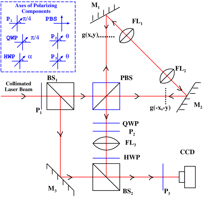
Figure 1: Recording geometry for combined FT holograms. The polarizing components and their orientations are shown in the top left corner in a dashed box.

Fig.1 and record optical CFT holograms. An expanded collimated beam of light from a He-Ne laser (red colored online) is split through a beam-splitter BS₁. One part is directed to a polarizing beam-splitter PBS. The two mirrors M₁ and M₂ form a triangular path interferometer, and the transmitted/reflected beams recombine by PBS. The transmissive object with amplitude transmittance $g(x,y)$ is placed inside the interferometer. We place one Fourier lens pair FL₁ and FL₂ of equal focal lengths inside the interferometer such that an inverted image of the object is formed as shown in Fig.1. The interferometric arrangement is so adjusted such that the object $g(x,y)$ and its inverted image $g(-x,-y)$ are equidistant from the beam-splitter PBS. So, one can get at the output side of the interferometer Fresnel propagated wave fields from (i) the object function $g(x,y)$ and from (ii) an inverted version of the object function, i.e., $g(-x,-y)$. A third Fourier lens FL₃ is also placed which produces the Fourier transforms of $g(x,y)$ and $g(-x,-y)$ with appropriate coefficients that depend on the phase relationship between the wave fields propagating through the interferometric arms. The orientations of the polarizing components are shown in a dashed box. Another part of the input beam from the laser, which is transmitted from the beam-splitter BS₁ and is reflected by the mirror M₃, superposes with object bearing beams after transmitting through another beam-splitter BS₂. To get a CFT hologram at the CCD plane, the phase differences between the beams are adjusted to $2\phi$ using polarization-induced phase deb:polaphase .

The input laser beam is polarized by the polarizer P₁ at angle $\pi/4$ to the $x$-axis, and may be represented by a Jones vector $\hat{E}$ as jones:calculus

$$\hat{E}=E_{0}\begin{bmatrix}1\\ 1\end{bmatrix}$$ (19)

$E_{0}$ being the amplitude. This polarized beam is split by the polarizing beam-splitter PBS into two orthognally polarized beam along the $x$-axis and $y$-axis, and the Jones matrices corresponding to the PBS along the $x$-axis and $y$-axis may be given by jones:calculus

$$P_{x}=\begin{bmatrix}1&0\\ 0&0\end{bmatrix}\ ,\ \ \ \ \ P_{y}=\begin{bmatrix}0&0\\ 0&1\end{bmatrix}$$ (20)

The reflected polarized beam, after a round trip through the cyclic interferometer gets reflected by the PBS and comes out at the output side. Similarly, the transmitted polarized component comes out of the PBS by transmission at the output side. It is to be noted that these two polarized beams carry the object transmittance information $g(x,y)$ and its inversion $g(-x,-y)$ by appropriate lens transformation inside the interferometer. These two orthogonally polarized image bearing beams face a quarter-wave retardation plate QWP whose slow axis makes an angle $\pi/4$ with the $x$-axis. Finally, these two polarized beams after passing through the quarter-wave plate will pass through an analyzer P₂ and the wave fields proceed towards the CCD camera. After Fourier transformation by the third lens, the vector wave field distribution at the CCD camera plane will be given by

$$\hat{G}_{PI}(u,v)=P(\theta)[C(\pi/4)P_{x}\hat{E}G(u,v)$$

$$+\ C(\pi/4)P_{y}\hat{E}G(-u,-v)]$$ (21)

where $P(\theta)$ represents the Jones matrix of the analyzer P₂, $C(\pi/4)$ represents the Jones matrix of the quarter-wave retardation plate, and are given by jones:calculus

$$P(\theta) = \begin{bmatrix}\cos^{2}\theta&\cos\theta\sin\theta\\ \sin\theta\cos\theta&\sin^{2}\theta\end{bmatrix}$$ (22)

$$C(\pi/4) = {1\over 2}\begin{bmatrix}1+i\ \ \ &\ \ \ 1-i\\ 1-i\ \ \ &\ \ \ 1+i\end{bmatrix}$$ (23)

Performing matrix multiplications, equation (21) can be expressed as

$$\hat{G}_{PI}(u,v)=\left[\exp\left\{i\left({\pi\over 4}-\theta\right)\right\}G(u,v)+\exp\left\{-i\left({\pi\over 4}-\theta\right)\right\}G(-u,-v)\right]$$

$$\times\left[\begin{array}[]{cc}\cos\theta\\ \sin\theta\end{array}\right]$$ (26)

where we have dropped off the constant amplitude factors. If we put $\theta=\pi/4-\phi$, the polarization-induced phase difference becomes $2\phi$, and equation (26) becomes equivalent to the field distribution given by equation (18) and is nothing but the CFT of the object function $g(x,y)$ except that it is linearly polarized. We can also identify the phase factors $\exp\{i(\pi/4-\theta)\}$ and $\exp\{-i(\pi/4-\theta)\}$ as the complex coefficients $a_{1}$ and $a_{2}$ respectively.

Finally, an analyzer P₃ should be placed before the CCD camera whose transmission axis makes an angle $\theta$ (same as P₂) with the $x$-axis. A half-wave plate HWP should also be placed after the Fourier lens FL₃ with its slow axis making an angle $\alpha$ ($\alpha\neq\theta$) with the $x$-axis, so as to keeping the amplitudes of the object waves reaching the CCD camera much smaller than the amplitude of the reference wave. This will help to ensure that $|R|^{2}\gg|G_{cft}|^{2}$. The object waves and the reference wave will transmit through the analyzer P₃ and interfere to form thd CFT hologram which can be recorded by the CCD camera.

6 Feasibility Simulations

Although the derivations of the earlier sections are shown for continuous combined Fourier transform, it can be shown that the results are valid for discrete combined Fourier transform as well. We have carried out proof-of-the-principle study using computer simulations by using GNU Octave gnu_octave . The object transparency is of 200x200 pixels size as shown in Fig.2(a).

        

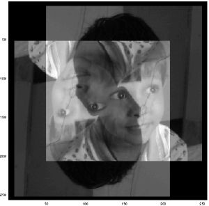
(a)                                                   (b)

        

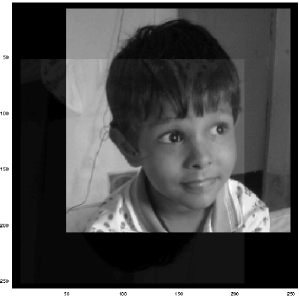
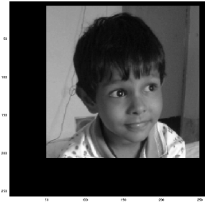
(c)                                                   (d)

Figure 2: Simulation results with a real object: (a) Object; Reconstruction from (b) FT hologram, (c) CFT hologram with $a_{1}\approx a_{2}^{\star}$, and (d) CFT hologram with $a_{1}=a_{2}^{\star}$.

The simulation window size is 256x256 pixels where the 200x200 pixels object is placed at the right hand top corner with zero padding. The object is purposefully off-centered so as to distinguish the twin reconstructions. The computational reconstruction of the object from a discrete FT hologram is carried out and is shown in Fig.2(b). Simulations for object reconstructions from the discrete CFT hologram can be done for two cases: Case I considering real object, and Case II considering complex object.

6.1 Case I: Reconstruction with a real object

This case is straight forward. Computational reconstructions from simulated discrete CFT holograms for different values of $a_{1}$ and $a_{2}$ are shown in Fig.2(c) and 2(d) for $a_{1}\approx a_{2}^{\star}$ ($b_{1}=1.7$, $b_{2}=1$) and for $a_{1}=a_{2}^{\star}$ ($b_{1}=b_{2}=1$) respectively. It is evident from Fig.2(b) that reconstruction of the FT hologram reproduces twin image with equal strengths. On the otherhand, for the CFT hologram, the effect of twin image is present for $a_{1}\neq a_{2}^{\star}$ ($b_{1}=1.7$, $b_{2}=1$), but the intensity levels of the two images are unequal [Fig.2(c)]. The effect of twin image is completely eliminated for $a_{1}=a_{2}^{\star}$ ($b_{1}=b_{2}=1$) as discernible from Fig.2(d). It is clear from the results of Fig.2(c) and Fig.2(d) that the effects of twin image in reconstructions of CFT holograms can be controlled by proper choice of $a_{1}$ and $a_{2}$, and can be completely eliminated for $a_{1}=a_{2}^{\star}$.

6.2 Case II: Reconstruction with a complex object

In practical situation the object would generally be complex, because the object transparency (either on glass plate or film) would have a phase variation due to variation in thickness or refractive index of the material or both. If $t(x,y)$ represents the thickness distribution over the object transparency, the phase distribution due to this thickness variation will be given by

$$\delta(x,y)=n\left({{2\pi}\over{\lambda}}\right)t(x,y)$$ (27)

where $\lambda$ is the wavelength of the laser and $n$ is the refractive index of the material of the transparency. Here, it is assumed that the refractive index of the material of the object transparency is uniform. We consider an example of a quadratic thickness variation, so $t(x,y)$ may be expressed as

$$t(x,y)=t_{0}+(x^{2}+y^{2})\Delta$$ (28)

where $t_{0}$ is the constant nominal thickness of the transparency plate and $\Delta$ is a thickness that is varied quadratically with spatial coordinates $x,y$. Therefore, the effect will be a phase factor $\exp[i\delta(x.y)]$ multiplied to the object function. If we put $\Delta=0$, we get a constant phase factor which is equivalent to the real object of Case I.

Simulations have been carried out with a 200x200 size phase function multiplied with the 200x200 size object function for $\lambda=633$ nm, $t_{0}=2$ mm and different values of $\Delta$, the overall simulation window remaining 256x256 size. The surface plot of the normalized phase function $t(x,y)$ for $\Delta=0$, and $\Delta=0.5\lambda$ are shown in Fig.3(a) and 3(b). The phase function profile is constant in Fig.3(a) which is nothing but the case of real object of Case I. The computational reconstructions of CFT holograms are shown in Fig.3(c), 3(d), 3(e) and 3(f) for $\Delta=0$, 0.5$\lambda$, $\lambda$ and 2$\lambda$ respectively. Here, the weighting multipliers are kept at $a_{1}=a_{2}^{\star}$ and $b_{1}=b_{2}=1$ for all. It is evident from Fig.3(c) – 3(f) that the phase variation of the object transparency gives rise to circular fringes modulated over the reconstructed object image. The effect is negligible for $\Delta=0.5\lambda$ [Fig.3(d)], but as $\Delta$ increases to $\lambda$, a circular fringe appears near the periphery of the image [Fig.3(e)]. When $\Delta=2\lambda$, the image is modulated by two circular fringes [Fig.3(f)]. It is clear that the thickness of the object transparency should be optically uniform, i.e., the surface finish of the object transparency plays an important role. That is why in such an interferometric arrangement, the object transparency may be placed inside an optical tank filled with an index matching liquid and optically polished glass windows with surface finish better than $\lambda/4$.

        

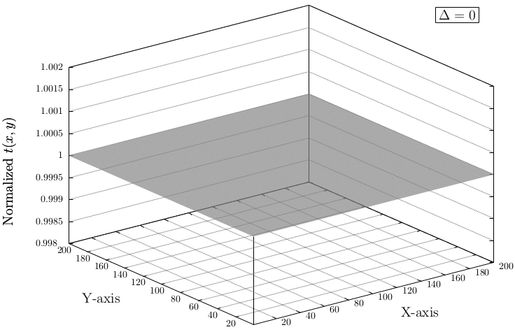
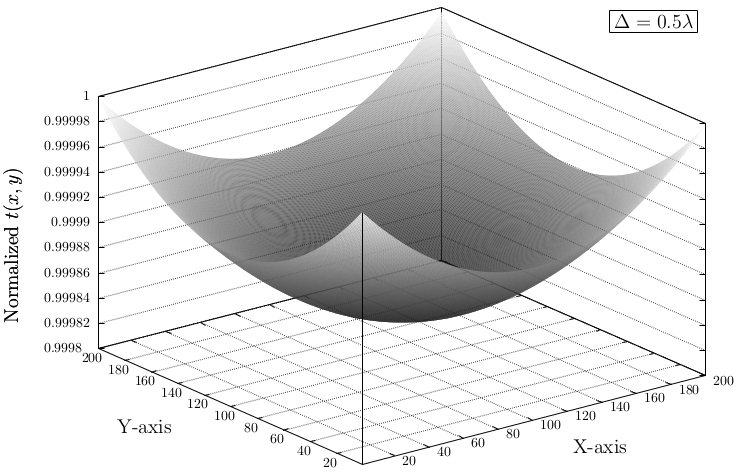
(a)                                                   (b)

        

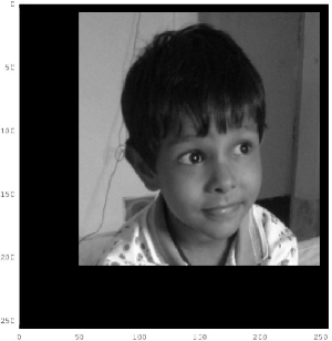
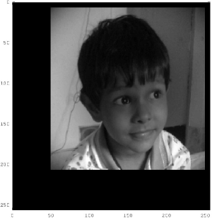
(c)                                                   (d)

        

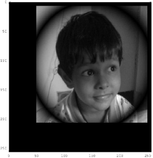
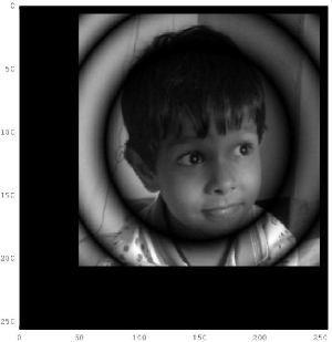
(e)                                                   (f)

Figure 3: Simulation results with a complex object: The normalized phase function $t(x,y)$ is shown for (a) $\Delta=0$ and (b) $\Delta=0.5\lambda$. Reconstructions from the CFT hologram are shown for (c) $\Delta=0$, (d) $\Delta=0.5\lambda$, (e) $\Delta=\lambda$ and (f) $\Delta=2\lambda$.

7 Discussions

The proof-of-the-principle simulations of the previous section proved the feasibility of twin image elimination in digital in-line holography using CFT. The proposed system is a polarization triangular path interferometer with a couple of Fourier lenses for synthesizing an inversion of the object function [$g(-x,-y)$], along with the object function [$g(x,y)$], and another Fourier lens for performing Fourier transform of the object and its inversion. The effect of CFT is created by introducing appropriate phase difference between the object information bearing waves by a polarization technique. Simulation is carried out for generating the CFT holograms for different values of the complex weighting factors. In this simulation, we have not considered the practical aspects of experimentation, such as effects of imperfections of the polarization components, aberrations of the Fourier lenses and the mirrors, misalignment errors of the interferometer, object wave to reference wave ratios and the quantization errors of the CCD camera.

The alignment of the proposed interferomeric system is not easy, nevertheless it is possible to implement combined Fourier transform optically. From equations (16), (17) and (18) it is evident that the complex constants $a_{1}$ and $a_{2}$ are transformed into a phase difference $2\phi$. So, in optical implementation, the constants $a_{1}$ and $a_{2}$ are not required to be specified directly, instead the orientations of the polarizing components are so adjusted such that the phase difference $2\theta$ between the two image bearing object waves can be made equal to $2\phi$. If one desires, one can easily express the induced phase differences equivalent to the complex factors $a_{1}$ and $a_{2}$ using De Moivre’s relations of equations (16) and (17). The complex coefficients $a_{1}$ and $a_{2}$ are also identified in the output of the interferometer in equation (26) as exponential phase factors.

Since, it is an interferometric transformation, the holographic reconstruction is sensitive to phase aberrations of the object transparency. Thus, this technique may be useful for carrying out studies of phase objects. A similar inverting triangular path polarization interferometer was indeed utilized for implementing optical Hartley transform experimentally debHT:jopt1997 . We wish to consider the practical aspects in a future experimental implemetation of the proposed method.

8 Conclusion

We have proposed a technique for resolving twin image problem of in-line digital Fourier holography. We use a combination of Fourier transforms to eliminate the unwanted twin image. The technique relies on interferometric addition of Fourier transforms of the object and its inversion with appropriate complex weighting coefficients, which are introduced through polarization-induced phase. Simulation results prove the feasibility of complete elimination of one of the twin image. Moreover, the technique is sensitive to phase aberrations of the object transparency, thereby providing a way for phase sensing holographic imaging. The proposed method neither involves recording of several phase shifted holograms, nor it requires any iteration for digital reconstruction, which may render it suitable for recording holograms of fast changing sequences as well as fast digital reconstruction of the recorded holograms.

- (1) D. Gabor, “A new microscopic principle,” Nature 161, 777-778 (1948).
- (2) W. L. Bragg and G. L. Rogers, “Elimination of the unwanted image in diffraction microscopy,” Nature 167, 190 (1951).
- (3) B. M. Hennelly, D. P. Kelly, N. Pandey, D. Monaghan, “Review of twin reduction and twin removal techniques in holography,” Proc. China-Ireland International Conference on Information and Communications Technologies, Maynooth, Ireland, Pages 241-245 (2009).
- (4) E. Leith and J. Upatnieks, “Wavefront reconstruction with continuous-tone objects,” JOSA 53 1377-1381 (1963).
- (5) R. Ansari, “An extension of the discrete Fourier transform,” IEEE Trans Circuits Sys. CAS-32 (6), 618-619 (1985).
- (6) D. Choudhury, P. N. Puntambekar and A. K. Chakraborty, “Utilization of polarization-induced phase difference for complex addition and subtraction of amplitudes,” J. Opt. 22, 6-10 (1993).
- (7) A. Gerald and J.M. Burch, Introduction to Matrix Methods in Optics (John Wiley & Sons, 1975).
- (8) GNU Octave: http://www.gnu.org/software/octave/ (accessed December 4, 2012)
- (9) D. Choudhury, P. N. Puntambekar and A. K. Chakraborty, “Hartley transformation by an inverting interferometer,” J. Opt. 26 (1997) 139-145.