Fast Training of Effective Multi-class Boosting Using Coordinate Descent Optimization

Abstract

We present a novel column generation based boosting method for multi-class classification. Our multi-class boosting is formulated in a single optimization problem as in [1, 2]. Different from most existing multi-class boosting methods, which use the same set of weak learners for all the classes, we train class specified weak learners (i.e., each class has a different set of weak learners). We show that using separate weak learner sets for each class leads to fast convergence, without introducing additional computational overhead in the training procedure. To further make the training more efficient and scalable, we also propose a fast coordinate descent method for solving the optimization problem at each boosting iteration. The proposed coordinate descent method is conceptually simple and easy to implement in that it is a closed-form solution for each coordinate update. Experimental results on a variety of datasets show that, compared to a range of existing multi-class boosting methods, the proposed method has much faster convergence rate and better generalization performance in most cases. We also empirically show that the proposed fast coordinate descent algorithm needs less training time than the MultiBoost algorithm in Shen and Hao [1].

1 Introduction

Boosting methods combine a set of weak classifiers (weak learners) to form a strong classifier. Boosting has been extensively studied [3, 4] and applied to a wide range of applications due to its robustness and efficiency (e.g., real-time object detection [5, 6, 7]). Despite that fact that most classification tasks are inherently multi-class problems, the majority of boosting algorithms are designed for binary classification. A popular approach to multi-class boosting is to split the multi-class problem into a bunch of binary classification problems. A simple example is the one-vs-all approach. The well-known error correcting output coding (ECOC) methods [8] belong to this category. AdaBoost.ECC [9], AdaBoost.MH [10] and AdaBoost.MO [10] can all be viewed as examples of the ECOC approach. The second approach is to directly formulate multi-class as a single learning task, which is based on pairwise model comparisons between different classes. Shen and Hao’s direct formulation for multi-class boosting (referred to as MultiBoost) is such an example [1]. From the perspective of optimization, MultiBoost can be seen as an extension of the binary column generation boosting framework [11, 4] to the multi-class case. Our work here builds upon MultiBoost. As most existing multi-class boosting, for MultiBoost of [1], different classes share the same set of weak learners, which leads to a sparse solution of the model parameters and hence slow convergence. To solve this problem, in this work we propose a novel formulation (referred to as MultiBoost_cw) for multi-class boosting by using separate weak learner sets. Namely, each class uses its own weak learner set. Compared to MultiBoost, MultiBoost_cw converges much faster, generally has better generalization performance and does not introduce additional time cost for training. Note that AdaBoost.MO proposed in [10] uses different sets of weak classifiers for each class too. AdaBoost.MO is based on ECOC and the code matrix in AdaBoost.MO is specified before learning. Therefore, the underlying dependence between the fixed code matrix and generated binary classifiers is not explicitly taken into consideration, compared with AdaBoost.ECC. In contrast, our MultiBoost_cw is based on the direct formulation of multi-class boosting, which leads to fundamentally different optimization strategies. More importantly, as shown in our experiments, our MultiBoost_cw is much more scalable than AdaBoost.MO although both enjoy faster convergence than most other multi-class boosting.

In MultiBoost [1], sophisticated optimization tools like Mosek or LBFGS-B [12] are needed to solve the resulting optimization problem at each boosting iteration, which is not very scalable. Here we propose a coordinate descent algorithm (FCD) for fast optimization of the resulting problem at each boosting iteration of MultiBoost_cw. FCD methods choose one variable at a time and efficiently solve the single-variable sub-problem. CD(coordinate decent) has been applied to solve many large-scale optimization problems. For example, Yuan et al. [13] made comprehensive empirical comparisons of $\ell_{1}$ regularized classification algorithms. They concluded that CD methods are very competitive for solving large-scale problems. In the formulation of MultiBoost (also in our MultiBoost_cw), the number of variables is the product of the number of classes and the number of weak learners, which can be very large (especially when the number of classes is large). Therefore CD methods may be a better choice for fast optimization of multi-class boosting. Our method FCD is specially tailored for the optimization of MultiBoost_cw. We are able to obtain a closed-form solution for each variable update. Thus the optimization can be extremely fast. The proposed FCD is easy to implement and no sophisticated optimization toolbox is required.

Main Contributions 1) We propose a novel multi-class boosting method (MultiBoost_cw) that uses class specified weak learners. Unlike MultiBoost sharing a single set of weak learners across different classes, our method uses a separate set of weak learners for each class. We generate $K$ (the number of classes) weak learners in each boosting iteration—one weak learner for each class. With this mechanism, we are able to achieve much faster convergence. 2) Similar to MultiBoost [1], we employ column generation to implement the boosting training. We derive the Lagrange dual problem of the new multi-class boosting formulation which enable us to design fully corrective multi-class algorithms using the primal-dual optimization technique. 3) We propose a FCD method for fast training of MultiBoost_cw. We obtain an analytical solution for each variable update in coordinate descent. We use the Karush-Kuhn-Tucker (KKT) conditions to derive effective stop criteria and construct working sets of violated variables for faster optimization. We show that FCD can be applied to fully corrective optimization (updating all variables) in multi-class boosting, similar to fast stage-wise optimization in standard AdaBoost (updating newly added variables only).

Notation Let us assume that we have $K$ classes. A weak learner is a function that maps an example ${\boldsymbol{x}}$ to $\{-1,+1\}$. We denote each weak learner by ${\hbar}$: ${\hbar}_{y,j}(\cdot,\cdot)\in{\operatorname{\mathcal{F}}},(y=1\dots K$, and $j=1\dots n$). ${\operatorname{\mathcal{F}}}$ is the space of all the weak learners; $n$ is the number of weak learners. We define column vectors ${\mathds{h}}_{y}({\boldsymbol{x}})=[{\hbar}_{y,1}({\boldsymbol{x}}),\cdots,{\hbar}_{y,n}({\boldsymbol{x}})]^{\!\top}$ as the outputs of weak learners associated with the $y$-th class on example ${\boldsymbol{x}}$. Let us denote the weak learners’ coefficients ${\boldsymbol{w}}_{y}$ for class $y$. Then the strong classifier for class $y$ is $F_{y}({\boldsymbol{x}})={\boldsymbol{w}}^{\!\top}{\mathds{h}}_{y}({\boldsymbol{x}})$. We need to learn $K$ strong classifiers, one for each class. Given a test data ${\boldsymbol{x}}$, the classification rule is $y^{\star}=\operatorname*{argmax\,}F_{y}({\boldsymbol{x}})$. ${\mathds{1}}$ is a vector with elements all being one. Its dimension should be clear from the context.

2 Our Approach

We show how to formulate the multi-class boosting problem in the large margin learning framework. Analogue to MultiBoost, we can define the multi-class margins associate with training data $({\boldsymbol{x}}_{i},y_{i})$ as

$$\gamma_{(i,y)}={\boldsymbol{w}}_{y_{i}}^{\!\top}{\mathds{h}}_{y_{i}}({\boldsymbol{x}}_{i})-{\boldsymbol{w}}_{y}^{\!\top}{\mathds{h}}_{y}({\boldsymbol{x}}_{i}),$$ (1)

for $y\neq y_{i}$. Intuitively, $\gamma_{(i,y)}$ is the difference of the classification scores between a “wrong” model and the right model. We want to make this margin as large as possible. MultiBoost_cw with the exponential loss can be formulated as:

$$\min_{{{\boldsymbol{w}}\geq 0,{\boldsymbol{\gamma}}}}\|{\boldsymbol{w}}\|_{1}+{\frac{C}{p}}\,\sum_{i}\sum_{y\neq y_{i}}\exp(-\gamma_{(i,y)}),\forall i=1\cdots m;\forall y\in\{1\cdots K\}\backslash y_{i}.$$ (2)

Here $\gamma$ is defined in (1). We have also introduced a shorthand symbol $p=m\times(K-1)$. The parameter ${C}$ controls the complexity of the learned model.

The model parameter is ${\boldsymbol{w}}=[{\boldsymbol{w}}_{1};{\boldsymbol{w}}_{2};\dots,{\boldsymbol{w}}_{K}]^{\!\top}\in\mathbb{R}^{K\cdot n\times 1}$.

Minimizing (2) encourages the confidence score of the correct label $y_{i}$ of a training example ${\boldsymbol{x}}_{i}$ to be larger than the confidence of other labels. We define $\operatorname{\mathcal{Y}}$ as a set of $K$ labels: $\operatorname{\mathcal{Y}}=\{1,2,\dots,K\}$. The discriminant function $F:\operatorname{\mathcal{X}}\times\operatorname{\mathcal{Y}}\mapsto\mathbb{R}$ we need to learn is: $F({\boldsymbol{x}},y;{\boldsymbol{w}})={\boldsymbol{w}}_{y}^{\!\top}{\mathds{h}}_{y}({\boldsymbol{x}})={\textstyle\sum}_{j}w_{(y,j)}{\hbar}_{(y,j)}({\boldsymbol{x}})$. The class label prediction $y^{\star}$ for an unknown example ${\boldsymbol{x}}$ is to maximize $F({\boldsymbol{x}},y;{\boldsymbol{w}})$ over $y$, which means finding a class label with the largest confidence: $y^{\star}=\operatorname*{argmax\,}_{y}F({\boldsymbol{x}},y;{\boldsymbol{w}})=\operatorname*{argmax\,}_{y}{\boldsymbol{w}}_{y}^{\!\top}{\mathds{h}}({\boldsymbol{x}}).$ MultiBoost_cw is an extension of MultiBoost [1] for multi-class classification. The only difference is that, in MultiBoost, different classes share the same set of weak learners ${\mathds{h}}$. In contrast, each class associates a separate set of weak learners. We show that MultiBoost_cw learns a more compact model than MultiBoost.

Algorithm 1 CG: Column generation for MultiBoost_cw

1: Input: training examples $({\boldsymbol{x}}_{1};y_{1}),({\boldsymbol{x}}_{2};y_{2}),\cdots$; regularization parameter $C$; termination threshold and the maximum iteration number.

2: Initialize: Working weak learner set $\operatorname{\mathcal{H}}_{c}=\emptyset(c=1\cdots K)$; initialize $\forall(i,y\neq y_{i}):\lambda_{(i,y)}=1$ ($i=1,\dots,m,y=1,\dots,K$).

3: Repeat

4:$\quad-$ Solve (2) to find $K$ weak learners: ${\hbar}_{c}^{\star}(\cdot),c=1\cdots K$; and add them to the working weak learner set $\operatorname{\mathcal{H}}_{c}$.

5:$\quad-$ Solve the primal problem (2) on the current working weak learner sets: ${\hbar}_{c}\in\operatorname{\mathcal{H}}_{c},c=1,\dots,K$.

to obtain ${\boldsymbol{w}}$ (we use coordinate descent of Algorithm 2).

6:$\quad-$ Update dual variables ${\boldsymbol{\lambda}}$ in (5) using the primal solution ${\boldsymbol{w}}$ and the KKT conditions (5).

7: Until the relative change of the primal objective function value is smaller than the prescribed tolerance; or the maximum iteration is reached.

8: Output: $K$ discriminant function $F({\boldsymbol{x}},y;{\boldsymbol{w}})={\boldsymbol{w}}_{y}^{\!\top}{\mathds{h}}_{y}({\boldsymbol{x}})$, $y=1\cdots K$.

Column generation for MultiBoost_cw To implement boosting, we need to derive the dual problem of (2). Similar to [1], the dual problem of (2) can be written as (3), in which $c$ is the index of class labels. $\lambda_{(i,y)}$ is the dual variable associated with one constraint in (2):

$$\max_{{\boldsymbol{\lambda}}}\;\; \sum_{i}\sum_{y\neq y_{i}}\lambda_{(i,y)}\big{[}1-\log\tfrac{p}{C}-\log\lambda_{(i,y)}\big{]}$$ (3a)

$${\rm s.t.}\;\; \forall c=1,\dots,K:$$

$$\sum_{i(y_{i}=c)}\sum_{y\neq y_{i}}\lambda_{(i,y)}{\mathds{h}}_{y_{i}}(\operatorname{\mathbf{x}}_{i})-\sum_{i}\sum_{y\neq y_{i},y=c}\lambda_{(i,y)}{\mathds{h}}_{y}(\operatorname{\mathbf{x}}_{i})\leq{\mathds{1}},$$ (3b)

$$\forall i=1,\dots,m:0\leq\sum_{y\neq y_{i}}\lambda_{(i,y)}\leq\tfrac{C}{p}.$$ (3c)

Following the idea of column generation [4], we divide the original problem (2) into a master problem and a sub-problem, and solve them alternatively. The master problem is a restricted problem of (2) which only considers the generated weak learners. The sub-problem is to generate $K$ weak learners (corresponding $K$ classes) by finding the most violated constraint of each class in the dual form (3), and add them to the master problem at each iteration. The sub-problem for finding most violated constraints can be written as:

$$\forall i= 1\cdots K:$$

$${\hbar}_{c}^{\star}(\cdot)=\operatorname*{argmax\,}_{{\hbar}_{c}(\cdot)}\sum_{i(y_{i}=c)}\sum_{y\neq y_{i}}\lambda_{(i,y)}{\mathds{h}}_{y_{i}}(\operatorname{\mathbf{x}}_{i})-\sum_{i}\sum_{y\neq y_{i},y=c}\lambda_{(i,y)}{\mathds{h}}_{y}(\operatorname{\mathbf{x}}_{i}).$$ (4)

The column generation procedure for MultiBoost_cw is described in Algorithm 1. Essentially, we repeat the following two steps until convergence: 1) We solve the master problem (2) with ${\hbar}_{c}\in\operatorname{\mathcal{H}}_{c},c=1,\dots,K$, to obtain the primal solution ${\boldsymbol{w}}$. $\operatorname{\mathcal{H}}_{c}$ is the working set of generated weak learners associated with the $c$-th class. We obtain the dual solution ${\boldsymbol{\lambda}}^{\star}$ from the primal solution ${\boldsymbol{w}}^{\star}$ using the KKT conditions:

$$\lambda_{(i,y)}^{\star}=\frac{C}{p}\exp\big{[}{\boldsymbol{w}}_{y}^{\star{\!\top}}{\mathds{h}}_{y}(\operatorname{\mathbf{x}}_{i})-{\boldsymbol{w}}_{y_{i}}^{\star{\!\top}}{\mathds{h}}_{y_{i}}(\operatorname{\mathbf{x}}_{i})\big{]}.$$ (5)

2) With the dual solution $\lambda_{(i,y)}^{\star}$, we solve the sub-problem (2) to generate $K$ weak learners: ${\hbar}_{c}^{\star},c=1,2,\dots,K$, and add to the working weak learner set $\operatorname{\mathcal{H}}_{c}$. In MultiBoost_cw, $K$ weak learners are generated for $K$ classes respectively in each iteration, while in MultiBoost, only one weak learner is generated at each column generation and shared by all classes. As shown in [1] for MultiBoost, the sub-problem for finding the most violated constraint in the dual form is:

$$[{\hbar}^{\star}(\cdot),\;c^{\star}]=\operatorname*{argmax\,}_{{\hbar}(\cdot),\;c}\sum_{i(y_{i}=c)}\sum_{y\neq y_{i}}\lambda_{(i,y)}{\mathds{h}}({\boldsymbol{x}}_{i})-\sum_{i}\sum_{y\neq y_{i},y=c}\lambda_{(i,y)}{\mathds{h}}({\boldsymbol{x}}_{i}).$$ (6)

At each column generation of MultiBoost, (6) is solved to generated one weak learner. Note that solving (6) is to search over all $K$ classes to find the best weak learner ${\hbar}^{\star}$. Thus the computational cost is the same as MultiBoost_cw. This is the reason why MultiBoost_cw does not introduce additional training cost compared to MultiBoost. In general, the solution $[{\boldsymbol{w}}_{1};\cdots;{\boldsymbol{w}}_{K}]$ of MultiBoost is highly sparse [1]. This can be observed in our empirical study. The weak learner generated by solving (6) actually is targeted for one class, thus using this weak learner across all classes in MultiBoost leads to a very sparse solution. The sparsity of $[{\boldsymbol{w}}_{1},\cdots,{\boldsymbol{w}}_{K}]$ indicates that one weak learner is usually only useful for the prediction of a very few number of classes (typically only one), but useless for most other classes. In this sense, forcing different classes to use the same set of weak learners may not be necessary and usually it leads to slow convergence. In contrast, using separate weak learner sets for each class, MultiBoost_cw tends to have a dense solution of ${\boldsymbol{w}}$. With $K$ weak learners generated at each iteration, MultiBoost_cw converges much faster.

Fast coordinate descent To further speed up the training, we propose a fast coordinate descent method (FCD) for solving the primal MultiBoost_cw problem at each column generation iteration. The details of FCD is presented in Algorithm 2. The high-level idea is simple. FCD works iteratively, and at each iteration (working set iteration), we compute the violated value of the KKT conditions for each variable in ${\boldsymbol{w}}$, and construct a working set of violated variables (denoted as $\mathcal{S}$), then pick variables from the $\mathcal{S}$ for update (one variable at a time). We also use the violated values for defining stop criteria. Our FCD is a mix of sequential and stochastic coordinate descent. For the first working set iteration, variables are sequentially picked for update (cyclic CD); in later working set iterations, variables are randomly picked (stochastic CD). In the sequel, we present the details of FCD. First, we describe how to update one variable of ${\boldsymbol{w}}$ by solving a single-variable sub-problem. For notation simplicity, we define: ${\delta}{\mathds{h}}_{i}(y)={\mathds{h}}_{y_{i}}({\boldsymbol{x}}_{i})\otimes\Gamma(y_{i})-{\mathds{h}}_{y}({\boldsymbol{x}}_{i})\otimes\Gamma(y).$ $\Gamma(y)$ is the orthogonal label coding vector: $\Gamma(y)=[\delta(y,1),\delta(y,2),\cdots,\delta(y,K)]^{\!\top}$ $\in\{0,1\}^{K}$. Here $\delta(y,k)$ is the indicator function that returns 1 if $y=k$, otherwise $0$. $\otimes$ denotes the tensor product. MultiBoost_cw in (2) can be equivalently written as:

$$\min_{{\boldsymbol{w}}\geq 0}\;\; \|{\boldsymbol{w}}\|_{1}+{\tfrac{C}{p}}\,\sum_{i}\sum_{y\neq y_{i}}\exp\big{[}-{\boldsymbol{w}}^{\!\top}{\delta}{\mathds{h}}_{i}(y)\big{]}.$$ (7)

We assume that binary weak learners are used here: ${\hbar}({\boldsymbol{x}})\in\{+1,-1\}$. ${\delta}{h}_{i,j}(y)$ denotes the $j$-th dimension of ${\delta}{\mathds{h}}_{i}(y)$, and ${\delta}{\bf\hat{\mathds{h}}}_{i,j}(y)$ denotes the rest dimensions of ${\delta}{\mathds{h}}_{i}(y)$ excluding the $j$-th. The output of ${\delta}{h}_{i,j}(y)$ only takes three possible values: ${\delta}{h}_{i,j}(y)\in\{-1,0,+1\}$. For the $j$-th dimension, we define: $\operatorname{\mathcal{D}}_{v}^{j}=\{\;(i,y)\;|\;{\delta}{h}_{i}^{j}(y)=v,i\in\{1,\dots,m\},y\in\operatorname{\mathcal{Y}}/y_{i}\;\},v\in\{-1,0,+1\}$; so $\operatorname{\mathcal{D}}_{v}^{j}$ is a set of constraint indices $(i,y)$ that the output of ${\delta}{h}_{i,j}(y)$ is $v$. $w_{j}$ denotes the $j$-th variable of ${\boldsymbol{w}}$; ${\bf\hat{{\boldsymbol{w}}}}_{j}$ denotes the rest variables of ${\boldsymbol{w}}$ excluding the $j$-th. Let $g({\boldsymbol{w}})$ be the objective function of the optimization (7). $g({\boldsymbol{w}})$ can be de-composited as:

$$g({\boldsymbol{w}}) =\|{\boldsymbol{w}}\|_{1}+{\tfrac{C}{p}}\sum_{i}\sum_{y\neq y_{i}}\exp\big{[}-{\boldsymbol{w}}^{\!\top}{\delta}{\mathds{h}}_{i}(y)\big{]}$$

$$=\|{\bf\hat{{\boldsymbol{w}}}}_{j}\|_{1}+\|w_{j}\|_{1}+{\tfrac{C}{p}}\sum_{i,y\neq y_{i}}\exp\big{[}-{\bf\hat{{\boldsymbol{w}}}}_{j}^{\!\top}{\delta}{\bf\hat{\mathds{h}}}_{i,j}(y)-w_{j}^{\!\top}{\delta}{h}_{i,j}(y)\big{]}$$

$$=\|{\bf\hat{{\boldsymbol{w}}}}_{j}\|_{1}+\|w_{j}\|_{1}+{\tfrac{C}{p}}\bigg{\{}\exp(w^{\!\top}_{j})\sum_{(i,y)\in\operatorname{\mathcal{D}}_{-1}^{j}}\exp\big{[}-{\bf\hat{{\boldsymbol{w}}}}_{j}^{\!\top}{\delta}{\bf\hat{\mathds{h}}}_{i,j}(y)\big{]}+$$

$$\quad\exp(-w^{\!\top}_{j})\sum_{(i,y)\in\operatorname{\mathcal{D}}_{+1}^{j}}\exp\big{[}-{\bf\hat{{\boldsymbol{w}}}}_{j}^{\!\top}{\delta}{\bf\hat{\mathds{h}}}_{i,j}(y)\big{]}+\sum_{(i,y)\in\operatorname{\mathcal{D}}_{0}^{j}}\exp\big{[}-{\bf\hat{{\boldsymbol{w}}}}_{j}^{\!\top}{\delta}{\bf\hat{\mathds{h}}}_{i,j}(y)\big{]}\bigg{\}}$$

$$=\|{\bf\hat{{\boldsymbol{w}}}}_{j}\|_{1}+\|w_{j}\|_{1}+{\tfrac{C}{p}}\big{[}\exp(w^{\!\top}_{j}){V}_{-}+\exp(-w^{\!\top}_{j}){V}_{+}+{V}_{0}\big{]}.$$ (8)

Here we have defined:

$${V}_{-}=\sum_{(i,y)\in\operatorname{\mathcal{D}}_{-1}^{j}}\exp\big{[}-{\bf\hat{{\boldsymbol{w}}}}_{j}^{\!\top}{\delta}{\bf\hat{\mathds{h}}}_{i,j}(y)\big{]}, \quad{V}_{0}=\sum_{(i,y)\in\operatorname{\mathcal{D}}_{0}^{j}}\exp\big{[}-{\bf\hat{{\boldsymbol{w}}}}_{j}^{\!\top}{\delta}{\bf\hat{\mathds{h}}}_{i,j}(y)\big{]},$$ (9a)

$${V}_{+}=\sum_{(i,y)\in\operatorname{\mathcal{D}}_{+1}^{j}}\exp\big{[}-{\bf\hat{{\boldsymbol{w}}}}_{j}^{\!\top}{\delta}{\bf\hat{\mathds{h}}}_{i,j}(y)\big{]}.$$ (9b)

In the variable update step, one variable $w_{j}$ is picked at a time for updating and other variables ${\bf\hat{{\boldsymbol{w}}}}_{j}$ are fixed; thus we need to minimize $g$ in (8) w.r.t $w_{j}$, which is a single-variable minimization. It can be written as:

$$\min_{w_{j}\geq 0}\;\; \|w_{j}\|_{1}+{\tfrac{C}{p}}\big{[}{V}_{-}\exp(w^{\!\top}_{j})+{V}_{+}\exp(-w^{\!\top}_{j})\big{]}.$$ (10)

The derivative of the objective function in (10) with $w_{j}>0$ is:

$$\frac{\partial g}{\partial w_{j}}=0\implies 1+\tfrac{C}{p}\big{[}{V}_{-}\exp(w^{\!\top}_{j})-{V}_{+}\exp(-w^{\!\top}_{j})\big{]}=0.$$ (11)

By solving (11) and the bounded constraint $w_{j}\geq 0$, we obtain the analytical solution of the optimization in (10) (since ${V}_{-}>0$):

$$w_{j}^{\star}=\max\bigg{\{}0,\;\;\log\bigg{(}\sqrt{{V}_{+}{V}_{-}+\tfrac{p^{2}}{4C^{2}}}-\tfrac{p}{2C}\bigg{)}-\log{{V}_{-}}\bigg{\}}.$$ (12)

When $C$ is large, (12) can be approximately simplified as:

$$w_{j}^{\star}=\max\bigg{\{}0,\;\;\frac{1}{2}\log\frac{{V}_{+}}{{V}_{-}}\bigg{\}}.$$ (13)

With the analytical solution in (12), the update of each dimension of ${\boldsymbol{w}}$ can be performed extremely efficiently. The main requirement for obtaining the closed-form solution is that the use of discrete weak learners.

We use the KKT conditions to construct a set of violated variables and derive meaningful stop criteria. For the optimization of MultiBoost_cw (7), KKT conditions are necessary conditions and also sufficient for optimality. The Lagrangian of (7) is: $L=\|{\boldsymbol{w}}\|_{1}+{\tfrac{C}{p}}\,\sum_{i}\sum_{y\neq y_{i}}\exp\big{[}-{\boldsymbol{w}}^{\!\top}{\delta}{\mathds{h}}_{i}(y)\big{]}-{\boldsymbol{\alpha}}^{\!\top}{\boldsymbol{w}}.$ According to the KKT conditions, ${\boldsymbol{w}}^{\star}$ is the optimal for (10) if and only if ${\boldsymbol{w}}^{\star}$ satisfies ${\boldsymbol{w}}^{\star}\geq 0,{\boldsymbol{\alpha}}^{\star}\geq 0,\forall j:\alpha^{\star}_{j}w^{\star}_{j}=0$ and $\forall j:\nabla_{j}L({\boldsymbol{w}}^{\star})=0$. For $w_{j}>0$,

$$\frac{\partial L}{\partial w_{j}}=0\implies 1-{\tfrac{C}{p}}\,\sum_{i}\sum_{y\neq y_{i}}\exp\big{[}-{\boldsymbol{w}}{\delta}{\mathds{h}}_{i}(y)\big{]}{\delta}{h}_{i,j}(y)-\alpha_{j}=0.$$

Considering the complementary slackness: $\alpha^{\star}_{j}w^{\star}_{j}=0$, if $w^{\star}_{j}>0$, we have $\alpha^{\star}_{j}=0$; if $w^{\star}_{j}=0$, we have $\alpha^{\star}_{j}\geq 0$. The optimality conditions can be written as:

$$\forall j:\left\{\begin{array}[]{l l}1-{\tfrac{C}{p}}\,\sum_{i}\sum_{y\neq y_{i}}\exp\big{[}-{\boldsymbol{w}}^{\star}{\delta}{\mathds{h}}_{i}(y)\big{]}{\delta}{h}_{i,j}(y)=0,&\quad\text{if $w_{j}^{\star}>0$};\\ 1-{\tfrac{C}{p}}\,\sum_{i}\sum_{y\neq y_{i}}\exp\big{[}-{\boldsymbol{w}}^{\star}{\delta}{\mathds{h}}_{i}(y)\big{]}{\delta}{h}_{i,j}(y)\geq 0,&\quad\text{if $w_{j}^{\star}=0$}.\\ \end{array}\right.$$ (14)

For notation simplicity, we define a column vector ${\boldsymbol{\mu}}$ as in (15). With the optimality conditions (14), we define ${\boldsymbol{\theta}}_{j}$ in (16) as the violated value of the $j$-th variable of the solution ${\boldsymbol{w}}^{\star}$:

$${\boldsymbol{\mu}}_{(i,y)}=\exp\big{[}-{\boldsymbol{w}}^{\!\top}{\delta}{\mathds{h}}_{i}(y)\big{]}$$ (15)

$${\boldsymbol{\theta}}_{j}=\left\{\begin{array}[]{l l}|1-{\tfrac{C}{p}}\,\sum_{i}\sum_{y\neq y_{i}}{\boldsymbol{\mu}}_{(i,y)}\,{\delta}{h}_{i,j}(y)|&\quad\text{if $w_{j}^{\star}>0$}\\ \max\{0,\;{\tfrac{C}{p}}\,\sum_{i}\sum_{y\neq y_{i}}{\boldsymbol{\mu}}_{(i,y)}\,{\delta}{h}_{i,j}(y)-1\}&\quad\text{if $w_{j}^{\star}=0$}.\\ \end{array}\right.$$ (16)

At each working set iteration of FCD, we compute the violated values ${\boldsymbol{\theta}}$, and construct a working set $\mathcal{S}$ of violated variables; then we randomly (except the first iteration) pick one variable from $\mathcal{S}$ for update. We repeat picking for $|\mathcal{S}|$ times; $|\mathcal{S}|$ is the element number of $\mathcal{S}$. $\mathcal{S}$ is defined as

$$\mathcal{S}=\{j\,|\,{\boldsymbol{\theta}}_{j}>\epsilon\;\}$$ (17)

where $\epsilon$ is a tolerance parameter. Analogue to [14] and [13], with the definition of the variable violated values ${\boldsymbol{\theta}}$ in (16), we can define the stop criteria as:

$$\max_{j}{\boldsymbol{\theta}}_{j}\leq\epsilon,$$ (18)

where $\epsilon$ can be the same tolerance parameter as in the working set $\mathcal{S}$ definition (17). The stop condition (18) shows if the largest violated value is smaller than some threshold, FCD terminates. We can see that using KKT conditions is actually using the gradient information. An inexact solution for ${\boldsymbol{w}}$ is acceptable for each column generation iteration, thus we place a maximum iteration number ($\tau_{max}$ in Algorithm 2) for FCD to prevent unnecessary computation. We need to compute ${\boldsymbol{\mu}}$ before obtaining ${\boldsymbol{\theta}}$, but computing ${\boldsymbol{\mu}}$ in (15) is expensive. Fortunately, we are able to efficiently update ${\boldsymbol{\mu}}$ after the update of one variable $w_{j}$ to avoid re-computing of (15). ${\boldsymbol{\mu}}$ in (15) can be equally written as:

$${\boldsymbol{\mu}}_{(i,y)}=\exp\big{[}-{\bf\hat{{\boldsymbol{w}}}}_{j}^{\!\top}{\delta}{\bf\hat{\mathds{h}}}_{i,j}(y)-w_{j}{\delta}{h}_{i,j}(y)\big{]}.$$ (19)

So the update of ${\boldsymbol{\mu}}$ is then:

$${\boldsymbol{\mu}}_{(i,y)}={\boldsymbol{\mu}}_{(i,y)}^{\text{old}}\exp\big{[}{\delta}{h}_{i,j}(y)(w_{j}^{\text{old}}-w_{j})\big{]}.$$ (20)

With the definition of ${\boldsymbol{\mu}}$ in (19), the values $V_{-}$ and $V_{+}$ for one variable update can be efficiently computed by using ${\boldsymbol{\mu}}$ to avoid the expensive computation in (9a) and (9b); $V_{-}$ and $V_{+}$ can be equally defined as:

$${V}_{-}=\sum_{(i,y)\in\operatorname{\mathcal{D}}_{-1}^{j}}{\boldsymbol{\mu}}_{(i,y)}\exp(-w_{j}), \quad{V}_{+}=\sum_{(i,y)\in\operatorname{\mathcal{D}}_{+1}^{j}}{\boldsymbol{\mu}}_{(i,y)}\exp(w_{j}).$$ (21)

Some discussion on FCD (Algorithm 2) is as follows: 1) Stage-wise optimization is a special case of FCD. Compared to totally corrective optimization which considers all variables of ${\boldsymbol{w}}$ for update, stage-wise only considers those newly added variables for update. We initialize the working set using the newly added variables. For the first working set iteration, we sequentially update the new added variables. If setting the maximum working set iteration to $1$ ($\tau_{max}=1$ in Algorithm 2), FCD becomes a stage-wise algorithm. Thus FCD is a generalized algorithm with totally corrective update and stage-wise update as special cases. In the stage-wise setting, usually a large $C$ (regularization parameter) is implicitly enforced, thus we can use the analytical solution in (13) for variable update.

2) Randomly picking one variable for update without any guidance leads to slow local convergence. When the solution gets close to the optimality, usually only very few variables need update, and most picks do not “hit”. In column generation (CG), the initial value of ${\boldsymbol{w}}$ is initialized by the solution of last CG iteration. This initialization is already fairly close to optimality. Therefore the slow local convergence for stochastic coordinate decent (CD) is more serious in column generation based boosting. Here we have used the KKT conditions to iteratively construct a working set of violated variables, and only the variables in the working set need update. This strategy leads to faster CD convergence.

Algorithm 2 FCD: Fast coordinate decent for MultiBoost_cw

1: Input: training examples $({\boldsymbol{x}}_{1};y_{1}),\cdots,({\boldsymbol{x}}_{m};y_{m})$; parameter $C$; tolerance: $\epsilon$ ; weak learner set $\operatorname{\mathcal{H}}_{c},c=1,\dots,K$; initial value of ${\boldsymbol{w}}$; maximum working set iteration: $\tau_{max}$.

2: Initialize: initialize variable working set $\mathcal{S}$ by variable indices in ${\boldsymbol{w}}$ that correspond to newly added weak learners; initialize ${\boldsymbol{\mu}}$ in (15); working set iteration index $\tau=0$.

3: Repeat (working set iteration)

4:       $\tau=\tau+1$; reset the inner loop index: $q=0$;

5:       While $q<|\mathcal{S}|$ ($|\mathcal{S}|$ is the size of $\mathcal{S}$)

6:             $q=q+1;$ pick one variable index $j$ from $\mathcal{S}$:

                         if $\tau=1$ sequentially pick one, else randomly pick one.

7:             Compute $V_{-}$ and $V_{+}$ in (21) using ${\boldsymbol{\mu}}$.

8:             update variable $w_{j}$ in (12) using $V_{-}$ and $V_{+}$.

9:             update ${\boldsymbol{\mu}}$ in (20) using the updated $w_{j}$.

10:       End While

11:       Compute the violated values ${\boldsymbol{\theta}}$ in (16) for all variables.

12:       Re-construct the variable working set $\mathcal{S}$ in (17) using ${\boldsymbol{\theta}}$.

13: Until the stop condition in (18) is satisfied or maximum working set iteration reached: $\tau>=\tau_{max}$.

14: Output: ${\boldsymbol{w}}$.

3 Experiments

We evaluate our method MultiBoost_cw on some UCI datasets and a variety of multi-class image classification applications, including digit recognition, scene recognition, and traffic sign recognition. We compare MultiBoost_cw against MultiBoost [1] with the exponential loss, and another there popular multi-class boosting algorithms: AdaBoost.ECC [9], AdaBoost.MH [10] and AdaBoost.MO [10]. We use FCD as the solver for MultiBoost_cw, and LBFGS-B [12] for MultiBoost. We also perform further experiments to evaluate FCD in detail. For all experiments, the best regularization parameter $C$ for MultiBoost_cw and MultiBoost is selected from $10^{2}$ to $10^{5}$; the tolerance parameter in FCD is set to $0.1$ ($\epsilon=0.1$); We use MultiBoost_cw-1 to denote MultiBoost_cw using the stage-wise setting of FCD which only uses one iteration ($\tau_{max}=1$ in Algorithm 2). In MultiBoost_cw-1, we fix $C$ to be a large value: $C=10^{8}$.

All experiments are run 5 times. We compare the testing error, the total training time and solver time on all datasets. The results show that our MultiBoost_cw and MultiBoost_cw-1 converge much faster then other methods, use less training time then MultiBoost, and achieve the best testing error on most datasets.

AdaBoost.MO [10] (Ada.MO) has a similar convergence rate as our method, but it is much slower than our method and becomes intractable for large scale datasets. We run Ada.MO on some UCI datasets and MNIST. Results are shown in Fig. 1 and Fig. 2. We set a maximum training time (1000 seconds) for Ada.MO; other methods are all below this maximum time on those datasets. If maximum time reached, we report the results of those finished iterations.

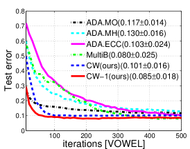
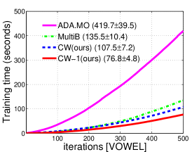
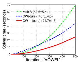
(a)

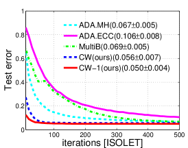
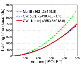
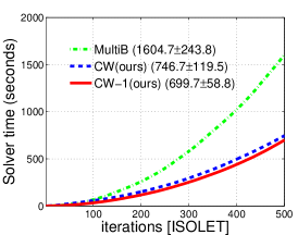
(b)

Figure 1: Results of 2 UCI datasets: VOWEL and ISOLET. CW and CW-1 are our methods. CW-1 uses stage-wise setting. The number after the method name is the mean value with standard deviation of the last iteration. Our methods converge much faster and achieve competitive test accuracy. The total training time and the solver time of our methods both are less than MultiBoost of [1].

UCI datasets: we use 2 UCI multi-class datasets: VOWEL and ISOLET. For each dataset, we randomly select 75% data for training and the rest for testing. Results are shown in Fig. 1.

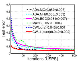
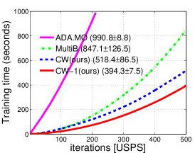
(a)

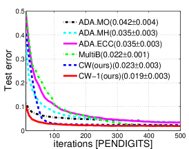
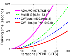
(b)

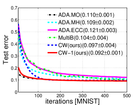
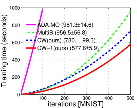
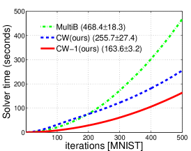
(c)

Figure 2: Experiments on 3 handwritten digit recognition datasets: USPS, PENDIGITS and MNIST. CW and CW-1 are our methods. CW-1 uses stage-wise setting. Our methods converge much faster, achieve best test error and use less training time. Ada.MO has similar convergence rate as ours, but requires much more training time. With a maximum training time of 1000 seconds, Ada.MO failed to finish 500 iterations on all 3 datasets.

Handwritten digit recognition: we use 3 handwritten datasets: MNIST, USPS and PENDIGITS. For MNIST, we randomly sample 1000 examples from each class, and use the original test set of 10,000 examples. For USPS and PENDIGITS, we randomly select 75% for training, the rest for testing. Results are shown in Fig. 2.

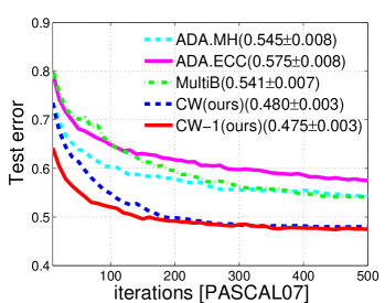
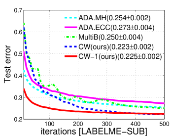
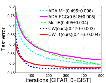
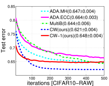
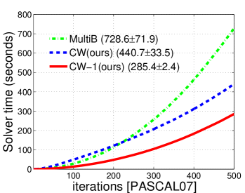
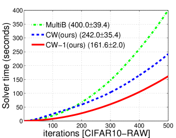
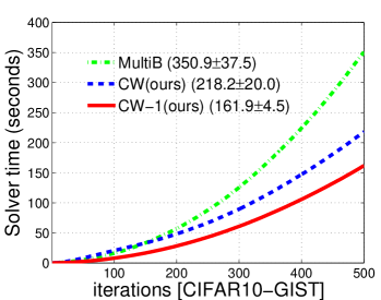
Figure 3: Experiments on 3 image datasets: PASCAL07, LabelMe and CIFAR10. CW and CW-1 are our methods. CW-1 uses stage-wise setting. Our methods converge much faster, achieve best test error and use less training time.

3 Image datasets: PASCAL07, LabelMe, CIFAR10: For PASCAL07, we use 5 types of features provided in [15]. For labelMe, we use the subset: LabelMe-12-50k and generate GIST features. For these two datasets, we use those images which only have one class label. We use 70% data for training, the rest for testing. For CIFAR10, we construct 2 datasets, one uses GIST features and the other uses the pixel values. We use the provided test set and 5 training sets for 5 times run. Results are shown in Fig. 3.

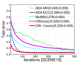
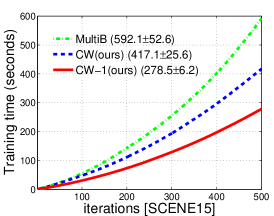
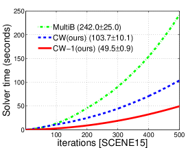
(a)

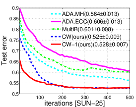
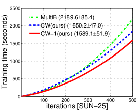
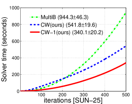
(b)

Figure 4: Experiments on 2 scene recognition datasets: SCENE15 and a subset of SUN. CW and CW-1 are our methods. CW-1 uses stage-wise setting. Our methods converge much faster and achieve best test error and use less training time.

Scene recognition: we use 2 scene image datasets: Scene15 [16] and SUN [17]. For Scene15, we randomly select 100 images per class for training, and the rest for testing. We generate histograms of code words as features. The code book size is 200. An image is divided into 31 sub-windows in a spatial hierarchy manner. We generate histograms in each sub-windows, so the histogram feature dimension is 6200. For SUN dataset, we construct a subset of the original dataset containing 25 categories. For each category, we use the top 200 images, and randomly select 80% data for training, the rest for testing. We use the HOG features described in[17]. Results are shown in Fig. 4.

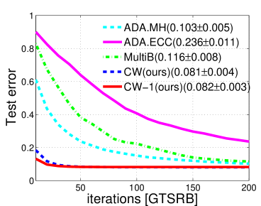
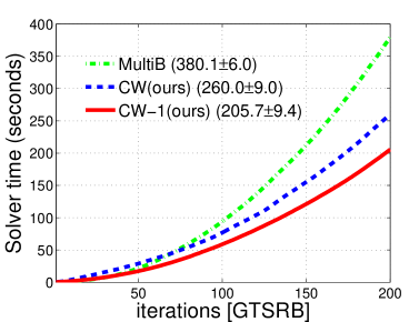
(a)

Figure 5: Results on the traffic sign dataset: GTSRB. CW and CW-1 (stage-wise setting) are our methods. Our methods converge much faster, achieve best test error and use less training time.

Traffic sign recognition: We use the GTSRB traffic sign dataset. There are 43 classes and more than 50000 images. We use the provided 3 types of HOG features; so there are 6052 features in total. We randomly select 100 examples per class for training and use the original test set. Results are shown in Fig.5.

3.1 FCD evaluation

We perform further experiments to evaluate FCD with different parameter settings, and compare to the LBFGS-B [12] solver. We use 3 datasets in this section: VOWEL, USPS and SCENE15. We run FCD with different settings of the maximum working set iteration($\tau_{max}$ in Algorithm 2) to evaluate how the setting of $\tau_{max}$ (maximum working set iteration) affects the performance of FCD. We also run LBFGS-B [12] solver for solving the same optimization (2) as FCD. We set $C=10^{4}$ for all cases. Results are shown in Fig. 6. For LBFGS-B, we use the default converge setting to get a moderate solution. The number after “FCD” in the figure is the setting of $\tau_{max}$ in Algorithm 2 for FCD. Results show that the stage-wise case ($\tau_{max}=1$) of FCD is the fastest one, as expected. When we set $\tau_{max}\geq 2$, the objective value of the optimization (2) of our method converges much faster than LBFGS-B. Thus setting of $\tau_{max}=2$ is sufficient to achieve a very accurate solution, and at the same time has faster convergence and less running time than LBFGS-B.

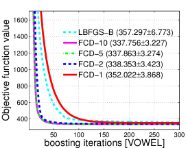
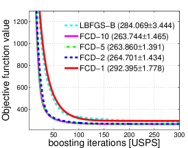
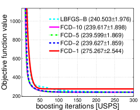
(a)

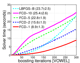
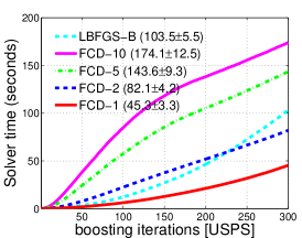
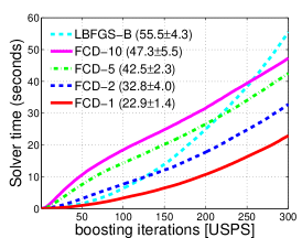
(b)

Figure 6: Solver comparison between FCD with different parameter setting and LBFGS-B [12]. One column for one dataset. The number after “FCD” is the setting for the maximum iteration ($\tau_{max}$) of FCD. The stage-wise setting of FCD is the fastest one. See the text for details.

4 Conclusion

In this work, we have presented a novel multi-class boosting method. Based on the dual problem, boosting is implemented using the column generation technique. Different from most existing multi-class boosting, we train a weak learner set for each class, which results in much faster convergence.

A wide range of experiments on a few different datasets demonstrate that the proposed multi-class boosting achieves competitive test accuracy compared with other existing multi-class boosting. Yet it converges much faster and due to the proposed efficient coordinate descent method, the training of our method is much faster than the counterpart of MultiBoost in [1].

Acknowledgement. This work was supported by ARC grants LP120200485 and FT120100969.

References

- [1] Shen, C., Hao, Z.: A direct formulation for totally-corrective multi-class boosting. In: Proc. IEEE Conf. Comp. Vis. Patt. Recogn. (2011)
- [2] Paisitkriangkrai, S., Shen, C., van den Hengel, A.: Sharing features in multi-class boosting via group sparsity. In: Proc. IEEE Conf. Comp. Vis. Patt. Recogn. (2012)
- [3] Schapire, R.E., Freund, Y., Bartlett, P., Lee, W.S.: boosting the margin: A new explanation for the effectiveness of voting methods. Annals of Statistics 26 (1998) 1651–1686
- [4] Shen, C., Li, H.: On the dual formulation of boosting algorithms. IEEE Trans. Pattern Anal. Mach. Intell. 32 (2010) 2216–2231
- [5] Viola, P., Jones, M.J.: Robust real-time face detection. Int. J. Comput. Vision 57 (2004) 137–154
- [6] Wang, P., Shen, C., Barnes, N., Zheng, H.: Fast and robust object detection using asymmetric totally-corrective boosting. IEEE Trans. Neural Networks & Learn. Syst. 23 (2012) 33–46
- [7] Paisitkriangkrai, S., Shen, C., Zhang, J.: Fast pedestrian detection using a cascade of boosted covariance features. IEEE Trans. Circuits & Syst. for Video Tech. 18 (2008) 1140–1151
- [8] Dietterich, T.G., Bakiri, G.: Solving multiclass learning problems via error-correcting output codes. J. Artif. Int. Res. 2 (1995) 263–286
- [9] Guruswami, V., Sahai, A.: Multiclass learning, boosting, and error-correcting codes. In: Proc. Annual Conf. Computational Learning Theory, New York, NY, USA, ACM (1999) 145–155
- [10] Schapire, R.E., Singer, Y.: Improved boosting algorithms using confidence-rated predictions. In: Machine Learn. (1999) 80–91
- [11] Demiriz, A., Bennett, K.P., Shawe-Taylor, J.: Linear programming boosting via column generation. Mach. Learn. 46 (2002) 225–254
- [12] Zhu, C., Byrd, R.H., Lu, P., Nocedal, J.: Algorithm 778: L-BFGS-B: Fortran subroutines for large-scale bound constrained optimization. ACM Trans. Math. Software (1994)
- [13] Yuan, G.X., Chang, K.W., Hsieh, C.J., Lin, C.J.: A comparison of optimization methods and software for large-scale l1-regularized linear classification. J. Mach. Learn. Res. (2010) 3183–3234
- [14] Fan, R.E., Chang, K.W., Hsieh, C.J., Wang, X.R., Lin, C.J.: LIBLINEAR: A library for large linear classification. J. Mach. Learn. Res. 9 (2008) 1871–1874
- [15] Guillaumin, M., Verbeek, J., Schmid, C.: Multimodal semi-supervised learning for image classification. In: Proc. IEEE Conf. Comp. Vis. Patt. Recogn. (2010)
- [16] Lazebnik, S., Schmid, C., Ponce, J.: Beyond bags of features: Spatial pyramid matching for recognizing natural scene categories. In: Proc. IEEE Conf. Comp. Vis. Patt. Recogn. Volume 2. (2006) 2169 – 2178
- [17] Xiao, J., Hays, J., Ehinger, K., Oliva, A., Torralba, A.: SUN database: Large-scale scene recognition from abbey to zoo. In: Proc. IEEE Conf. Comp. Vis. Patt. Recogn. (2010) 3485 –3492