Simulation and Analysis of TE Wave Propagation for Measurement of Electron Cloud Densities in Particle Accelerators

Abstract

The use of transverse electric (TE) waves has proved to be a powerful, noninvasive method for estimating the densities of electron clouds formed in particle accelerators. Results from the plasma simulation program VSim have served as a useful guide for experimental studies related to this method, which have been performed at various accelerator facilities. This paper provides results of the simulation and modeling work done in conjunction with experimental efforts carried out at the Cornell electron storage ring “Test Accelerator” (CesrTA). This paper begins with a discussion of the phase shift induced by electron clouds in the transmission of RF waves, followed by the effect of reflections along the beam pipe, simulation of the resonant standing wave frequency shifts and finally the effects of external magnetic fields, namely dipoles and wigglers. A derivation of the dispersion relationship of wave propagation for arbitrary geometries in field free regions with a cold, uniform cloud density is also provided.

1 Introduction

Electron clouds formed in circular particle accelerators with positively charged beams are known to degrade the quality of the beam. They are a concern for future accelerator facilities such as the International Linear Collider (ILC) damping rings, the SuperKEKB, and also upgrade of existing facilities such as the Large Hadron Collider (LHC) and the Fermilab Main Injector (MI). Their study is also important for the optimum performance of spallation neutron sources.

The detection of electron clouds has been a topic of study ever since their effects were first observed. The methods used for such a detection have included retarding field analyzers, clearing electrodes, shielded pickup detectors, TE waves and study of the response of the beam in the presence of an electron cloud. The TE wave method involves transmitting microwaves through a section of the beam pipe, and then studying the effect of the cloud on the microwave properties. The microwaves can be introduced either as traveling or standing waves within a section of the beam pipe.

The method of using microwaves as a probe for investigating the presence of electron clouds was first proposed by F. Caspers [1, 2], in which experiments were conducted at the SPS at CERN based on this method. The measurement technique involves measuring the height of modulation side-bands off the carrier frequency of the microwave. The electron cloud, constituting a plasma modifies the dispersion relationship of the microwave. The periodic production and clearing of the cloud, based on the bunch train passage frequency, leads to modulation of the phase advance of carrier wave as it travels. This modulation gives rise to side bands in the spectrum of the propagated wave. The side bands are spaced from the carrier frequency by a value equal to integer multiples of the train passage frequency. The details of the distribution of all the side band heights depends upon the nature of the build up and decay of the cloud. The study of this paper is restricted to the effect of the wave dispersion from a static cloud under various conditions. A confirmation of the electron cloud induced modulation was shown in the PEP II Low Energy Ring (LER) [3]. In this experiment, the wave was transmitted across a solenoidal section of the ring and the cloud density was controlled by adjusting the strength of the solenoidal magnetic field. The estimations of the electron cloud density in this experiment, done based on the formulation given in [4], were reasonable when compared to earlier build up simulations.

As shown in this paper, reflections within the beam pipe can alter the signal and thus misrepresent the cloud density in the region being sampled. Instead of transmitting the wave at a point and receiving it from another called traveling wave RF diagnostics, one could also trap the wave within a section called resonant wave RF diagnostics. This has the advantage that one can sample a known section of the beam pipe. This method would not be affected by waves being reflected from other segments of the pipe coming back into the section of interest and thus compromising the precision of the measurement. Another advantage of trapping, is that there is an enhancement of the signal as long as the point of measurement is close to a peak of the standing wave. Additionally, at resonance, as demonstrated in Ref [5], there is improved matching of the signal transfer from the electrodes into the waveguide, which is the beam pipe. As discussed in Ref [6], the modulation of the cloud density would result in a modulation of the resonant frequency enabling one to relate the frequency modulation signal to an actual cloud density. The draw back of this technique is the need for having reflectors at both ends of the desired section.

The electron cloud induced phase shift is known to undergo an enhancement in the presence of an external magnetic field under certain conditions, due to a modification in the dispersion relationship. This occurs when the wave magnetic field has a component perpendicular to the external magnetic field, and the frequency of the wave is close to the electron cyclotron frequency, corresponding to the value of the external magnetic field. This effect was demonstrated through simulations [7, 8], and was later confirmed through experiments done at PEP II across a chicane [9]. Further measurements done at the same chicane, now installed in CesrTA also confirm this effect. While it is good to have an enhanced signal, the drawback of such a measurement is that there is no available formulation that relates the enhanced side-band amplitude with the expected electron cloud density. In addition, as discussed in this paper, the phase shift progressively reduces as the electron cyclotron frequency exceeds the carrier wave frequency and at very high external magnetic fields the signal may not be observable at all. On can suppress the effect of the external magnetic field by aligning the wave electric field parallel to the external magnetic field, however it will be shown in this paper that this cannot be fully eliminated unless the waveguide is rectangular.

The program VSim[10], previously Vorpal, was used throughout to perform the simulations. The simulations used electromagnetic particle-in-cell (PIC) algorithms, consisting of propagating waves through a conducting beam pipe. The end of the pipe had perfectly-matched layers (PMLs) [7] meant to absorb any transmissions, and thus simulate a long, continuous beam pipe. Electrons were uniformly distributed and set to initially have zero velocity (a cold plasma). Waves were excited in the simulations with the help of a vertically pointing current density near one end of the beam pipe, which covered the full cross-sectional area and was two cells thick in the longitudinal dimension. In later simulations the PMLs and RF current source were replaced with port boundary conditions that simultaneously absorb RF energy at a single frequency at the ends of the simulation while also launching RF energy into the simulation domain to simulate traveling waves.

The waves were propagated along the channel using the Yee [5] algorithm for solving the electromagnetic field equations. The computational parameters used did not change much between the various simulations performed in this paper. All the simulations were three dimensional using a Cartesian grid. The grid sizes were around $2-3\mbox{mm}$ in each direction, the time steps varied between $2-4\times 10^{-12}s$. The macro-particles-per-cell used was typically 10, and they were loaded uniformly in position space, with zero initial velocity, often referred to as a “cold start”. The duration of the simulation was about 140 RF cycles.

Overall, the modeling effort related to measuring electron clouds using TE waves has served as a useful guide toward better understanding of the physical phenomenon and proper interpretation of the measured data. This paper provides a comprehensive account of simulations performed for various techniques currently under study. A derivation of the wave dispersion relationship for propagation through a beam pipe with a cold, uniform electron distribution in a field free region is given in the Appendix.

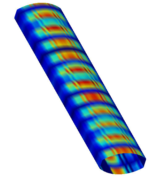
Figure 1: Snapshot of a Vorpal simulation showing propagation of a TE wave through the CesrTA beam pipe

2 Electron Cloud induced Phase shift from Transmission Through Field-Free regions and the effect of reflections

The first experiments using microwaves to assess the cloud densities involved simply transmitting the wave using a beam position monitor (BPM) and receiving the transmitted wave from another BPM downstream to the traveling wave [1, 3]. As shown in Ref [4], the electron cloud induced phase shift per unit length of transmission in the absence of external magnetic fields and a uniform electron distribution, can be related to the electron density as follows,

$$\Delta\phi=\frac{\omega_{p}^{2}}{2c(\omega^{2}-\omega_{co}^{2})^{1/2}}$$ (1)

where $\omega_{co}$ is the angular cutoff frequency for a waveguide in vacuum, $\omega_{p}=\sqrt{n_{e}e^{2}/\epsilon_{0}m_{e}}$ is the angular plasma frequency, with $n_{e}$ the electron number density, $e$ the charge of the electron, $c$ the speed of light, $m_{e}$ the electron mass and $\epsilon_{0}$ the free space permitivity. In Ref [4], this formula was validated through simulations for a square cross section beam pipe. The derivation of the phase shift given by Eq 1 used the dispersion relationship given in Ref [11],

$$k^{2}=\frac{\omega^{2}}{c^{2}}-\frac{\omega_{p}^{2}}{c^{2}}-\frac{\omega_{co}^{2}}{c^{2}}$$ (2)

which was proved to be valid for a circular waveguides free of external magnetic fields. The results shown in this paper validates the formula for a Cesr beam pipe geometry. All these results collectively indicate that the formula is valid for any type of geometry. In the Appedix, we provide an explicit proof that this is indeed the case. The Cesr beam pipe geometry may be represented in the form of two circular arcs (radius 0.075m) connected with flat side planes. It is about 0.090m from side to side and 0.050m between the apices of the arcs. The cutoff frequency of lowest mode for this geometry is known to be around $1.888$ GHz from past experiments and calculations related to the beam pipe. Figure 1 provides a snapshot of the simulation, showing the propagation of a wave through the Cesr beam pipe.

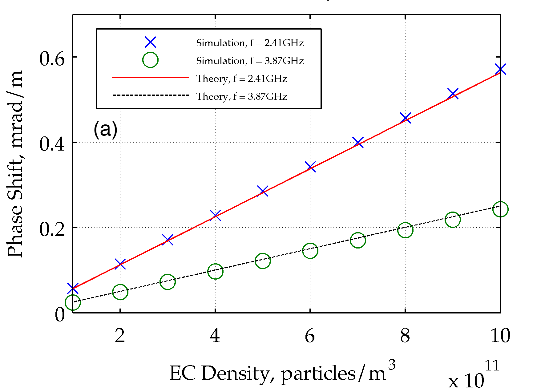
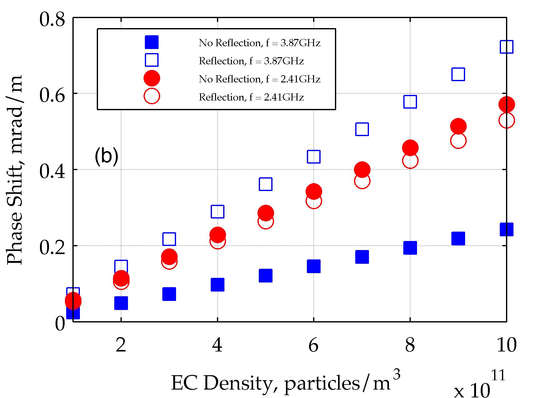
Figure 2: Variation of (a) phase shift with cloud density for a Cesr beam pipe geometry, and (b)the effect of reflections on the phase shift

Calculation of electron induced phase shift was performed through separate simulations of the wave transmission through a vacuum beam pipe and through a beam pipe with electrons respectively. At a certain axial distance $L$ from the location at which the wave was launched, the variation of the voltage between the midpoints of the top and bottom boundaries of the beam pipe cross section were recorded as a function of time. After normalizing the amplitudes of the two waves to unity, their difference gives a sinusoidal wave with an amplitude equal to the phase shift between the waves. Suppose that the angular frequency of the wave is $\omega$ and phase shift is $\delta$. The phase shift for nominal cloud densities is small enough that $\sin(\delta)\approx\delta$. Hence we have $\cos(\omega t)-\cos(\omega t+\delta)\approx\delta\sin(\omega t+\delta/2)$. The amplitudes of all the waves were calculated from their respective numerical RMS values.

To confirm the relationship between the phase shift and electron cloud density, simulations were done with a Cesr beam pipe with a length of 0.5m. Figure 2(a) shows that simulations agree well with the analytically predicted values given by Eq 1. This establishes the accuracy of the simulation method as well as the validity of Eq 1 for any geometry. We see that the electron cloud induced phase shift increases as one approaches the cutoff frequency. While this is desirable because it amplifies the modulation side-bands relative to the carrier signal, one will encounter reduced transmission as the carrier frequency approaches the cutoff.

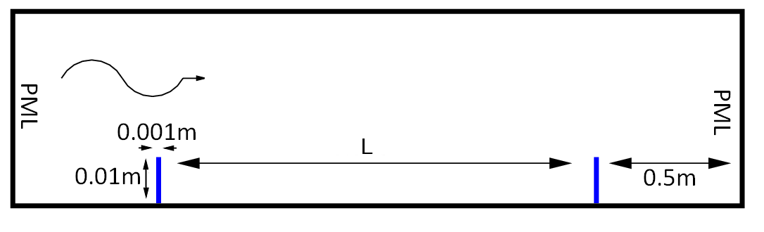
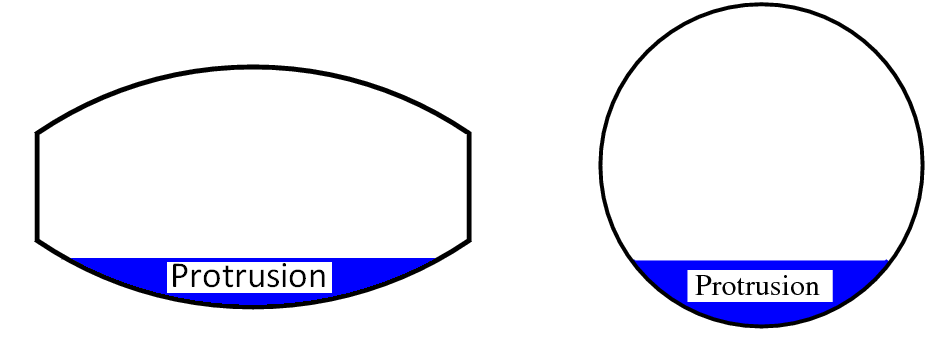
Figure 3: A schematic of the simulations with protrusions serving as partial reflectors, showing the Cesr and a circular cross section beam pipes. The latter geometry is used in Sec. 3

Due to the presence of several mechanical and electronic components all along the vacuum chamber, it is not very likely that one can perform phase shift experiments that are entirely free of internal reflections. As discussed in Ref [14], in an experiment, these internal reflections would potentially affect the value of the phase shift. A wave reflected from a device that lies beyond the segment being measured, would be received by the detector when it comes back after reflection. At the same time, waves could get reflected back and forth within the segment before eventually being received at the detector. In both cases, the reflected wave would have sampled a length different from that meant to be sampled and would thereby contaminate the signal, because the phase shift is proportional to the length of transmission. In order to understand this effect, the simulations were altered to include two protruding conductors, which would reflect some of the transmitted wave. The protrusions were slabs in the transverse plane, extending from the bottom to 1cm above the apex of the lower arc (see Fig. 3). They were spaced 0.4 meters apart, including the thickness of the protrusions, which was 1mm. The frequencies used for this study 2.41 GHz and 3.87 GHz, the same as those shown in Fig 2(a), correspond to the resonant harmonics ($n=4$ and $n=9$, respectively) of a 0.4 meter “resonant cavity”. This was done in order to maximize reflections. Fig. 2(b) shows the resulting phase shifts from these calculations. The solid shapes represent the data for no reflections and are the same data that appear in Fig. 2(a). The open shapes represent the phase shifts in the presence of reflection. These results clearly indicate that internal reflections modify the expected phase shift. The nature of the alteration of phase shift depends upon the complexities of the transmission-reflection combination, and the instrumentation used for the method. However, the results show that the linear relationship between phase shift and electron density is always preserved.

3 Standing Waves from Partial Reflectors and Electron Cloud Induced Resonant Frequency Shift

While internal reflections may interfere with phase shift measurements, they can also be used to trap a wave. This trapped wave can be used to measure the electron cloud density, as discussed in Ref [6]. This section shows the results of numerical simulation of such an experiment. The geometries used were (a) Cesr beam pipe also used in the previous section and (b) beam pipe with a circular cross section of radius 4.45cm. Both of them had conducting protrusions that were 1mm thick and 1cm high from the base as shown in Fig 3. The cutoff frequency for the circular beam pipe can be calculated from the analytic expression, and is 1.9755GHz for the lowest ($TE_{11}$) mode.

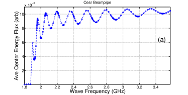
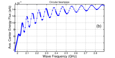
Figure 4: The average energy flux calculated over a range of frequencies, with the local minima indicating resonance points for (a) the Cesr beam pipe, (b) beam pipe with circular cross section

A trapped mode results when standing waves are induced between the reflectors. In order to test the effectiveness of inducing such a standing wave using partial reflectors, simulations were done with an empty wave guide over a large range of frequencies. It should be noted that, since there is only a partial reflection of the wave taking place, there is always a net transmission of energy across the segment between the protrusions. The wave energy that escapes the partial reflectors gets absorbed into the PML regions. Identification of a resonance was done as follows. At each frequency and each time step, the wave energy flux was computed by integrating the Poynting vector across a plane located at the mid point between the two protrusions. This plane was oriented transverse to the axis and covered the entire cross section. For each of these frequencies, the mean of the energy flux was calculated over the period of the simulation. It is expected that as the frequency approaches that of a standing wave, this averaged flux would reach a local minimum. This is because of increased ”back and forth” transmission which does not contribute to the average flux due to cancellation.

Figure 4 shows the average energy flux calculated for a variety of frequencies spanning over several resonance points for (a) the Cesr beam pipe (b) the circular cross section beam pipe. The local minima seen on these plots correspond to a standing wave mode. The length of the section, including the width of the protrusions was 0.4m for the Cesr beam pipe. The length of the circular beam pipe, including the width of the protrusions was 0.88m

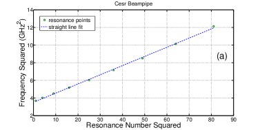
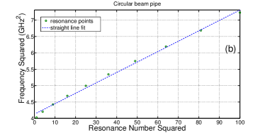
Figure 5: Resonance points obtained from the data in Fig 4 showing the linear relationship between $f_{0}^{2}$ and $n^{2}$ according to Eq 3

A standing wave occurs when the wavelength $\lambda$ and the length $L$ of the segment are related such that for any integer $n$, $L=n\lambda/2$. The dipersion relationship of a waveguide with wave frequency $f_{0}$ and cutoff frequency $f_{co}$, is given by $c^{2}/\lambda^{2}=f_{0}^{2}-f_{co}^{2}$. Expressing $\lambda$ in terms of $L$, for the standing wave, this then gives

$$f_{0}^{2}=\frac{c^{2}}{4L^{2}}n^{2}+f_{co}^{2}$$ (3)

This indicates the linear relationship between $f_{0}^{2}$ and $n^{2}$, and also the relationship of $L$ with the slope, and $f_{co}$ with the intercept of the straight line. Equation (3) was used to confirm that the local minima in Fig 4 correspond to resonance points. Figure 5 shows the value of $f_{0}^{2}$ plotted as a function of the corresponding value of $n^{2}$ for (a) the Cesr beam pipe and (b) beam pipe with a circular cross section. Performing a straight line fit on these points for case (a), yielded the relationship $f^{2}(GHz^{2})=0.104n^{2}+3.515$. This gives $L=0.465m$ and $f_{co}=1.875GHz$. For case (b), a similar operation gives $f_{0}^{2}(GHz^{2})=0.0318n^{2}+4.1276$ giving $L=0.841m$ and $f_{co}=2.0316GHz$. These values are close enough to the expected ones and ascertain the accuracy of such a method in determining standing waves between partial reflectors.

The presence of an electron cloud would result in a shift in the standing wave frequency. Experimentally, it is possible to measure this in the form of frequency modulation side-bands associated with the periodic passage of a train of bunches creating electron clouds. Using, Eq (2) we can show that the condition for standing waves given by Eq (3) is modified by an electron cloud as follows,

$$f_{e}^{2}=\frac{c^{2}}{4L^{2}}n^{2}+f_{co}^{2}+f_{p}^{2}$$ (4)

where the wave frequency is now denoted by $f_{e}$ and $f_{p}$ is the plasma frequency. Subtracting Eq 3 from Eq 4, and in the limit of small frequency shifts, we get, $f_{e}^{2}-f_{0}^{2}\approx 2\Delta ff_{0}=f_{p}^{2}$, where $\Delta f=f_{e}-f_{0}$. On inserting the expression for $f_{p}$, this then gives a simple expression relating the shift in resonant frequency as a function of electron density.

$$\Delta f=\frac{n_{e}e^{2}}{8\epsilon_{0}m_{e}\pi^{2}f_{0}}=\frac{n_{e}r_{e}c^{2}}{2\pi f_{0}}$$ (5)

in which $r_{e}$ is the classical electron radius. This shows that the frequency shift is proportional to the electron cloud density.

An effort is underway at CesrTA to use this method to measure the density of the electron cloud within the beam pipe section where the reflections are occurring [15]. Thus, it became necessary to test this phenomenon with simulations. Simulation of the frequency shift of standing waves was done for a Cesr beam pipe cross section as well as a beam pipe with a circular cross section. All the parameters were the same as before except that the length of the section between the partial reflectors for the Cesr beam pipe was modified from 0.4m to 0.9 m, which was somewhat close to one the setups under study at CesrTA. The length of the circular cross section was retained at 0.88m. Since the frequency shift induced by electrons is very small, it is required that the resonant frequency be determined accurately. To do this, a parabolic fit was made to the averaged energy flux in the vicinity of the minimum point, using the available points obtained from simulation. The expression for the parabola may be obtained from a Taylor expansion of the function around the minimum. This gives the mean energy flux as a function of frequency $f$ near the $n$th minimum point $f_{n}$. Thus, we have

$${\cal E}(f)={\cal E}^{\prime\prime}(f_{n})f^{2}-{\cal E}^{\prime\prime}(f_{n})f_{n}f+[{\cal E}(f_{n})+{\cal E}^{\prime\prime}(f_{n})f_{n}^{2}]$$ (6)

where ${\cal E}(f)$ is the averaged energy flux, ${\cal E}^{\prime\prime}(f_{n})$ is the second derivative of ${\cal E}$ evaluated at $f_{n}$. The first derivative of ${\cal E}$ at the minimum point vanishes. Using the computed coefficients of the parabola one can solve for $f_{n}$.

Figure 6 shows the frequency shift induced by electron clouds for the $n=2$ mode for (a) the Cesr beam pipe and the (b) the circular beam pipe. For case (a), the electron density used in this calculation was $10^{14}$ m^-3, which is rather high, but helps validate Eq (5) with simulations more accurately. For these parameters, the $n=2$ resonance occurs at 2.0033 GHz and the expected frequency shift due to electrons is 2 MHz. Simulations show a shift of 2.05 MHz. For case (b), we used two values of electron densities, $10^{14}$ m^-3 and $2\times 10^{14}$ m^-3. The expected frequency shift for the $10^{14}$ m^-3 case is 2.013MHz. The simulated frequency shift for this was 2.1MHz, and for an electron density of $2\times 10^{14}$ m^-3, it was 4.2MHz. Thus we were able to establish that reasonably accurate values of frequency shift for such an experiment may be determined from simulations. It is interesting to note that the error obtained in the resonant frequency itself was around $2MHz$, however the shift induced by electron clouds always had reasonable agreement with Eq 5. The agreement with theory provides confidence in estimating electron densities based on Eq 5 from measurements. Typical electron cloud densities are of the order of $10^{12}$m^-3 leading to frequency shifts about a factor of 100 smaller than those simulated here. Simulating frequency shifts this small would in principle be possible by scaling all numerical parameters appropriately, but this would have been a far more intensive computational process. However, it is well known that in practice, such small frequency modulations can be easily measured with standard spectrum analyzers.

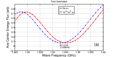
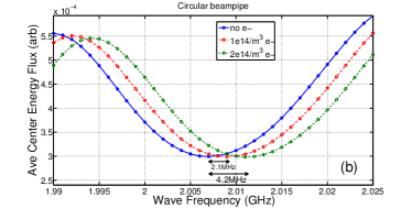
Figure 6: Simulation results showing a shift in the $n=2$ resonance frequency induced by electron clouds in (a) the Cesr beam pipe and (b) the circular cross section beam pipe.

4 Transmission and Phase Shift Through Dipole and Wiggler Field Regions

This section discusses the effect of external dipole and wiggler magnetic fields on the phase shift measurements. Simulations done in the past, have revealed that the phase shift is greatly amplified in the presence of an external magnetic field if the electron cyclotron frequency lies in the vicinity of the carrier frequency [7, 8]. Following these results, the cyclotron resonance was soon confirmed at an experiment performed at the SLAC chicane [9]. The SLAC chicane has since been transferred to CesrTA, where these studies continue to be made [16].

In the presence of an external magnetic field and electron clouds, the medium is no longer isotropic and the polarization of the transmitted microwave plays an important role in the outcome of the measurement. When the wave electric field is oriented perpendicular to the external magnetic field, the mode is referred to as an Extraordinary wave or simply X-wave. In this situation, if the external dipole field corresponds to an electron cyclotron frequency close to the carrier wave frequency, we see an enhanced phase shift. The phenomenon is well understood in the case of open boundaries. It is usually referred to as upper hybrid resonance. The dispersion relationship for the open boundary case is given as follows (see for example ref [17]).

$$\frac{c^{2}k^{2}}{\omega^{2}}=1-\frac{\omega_{p}^{2}(\omega^{2}-\omega_{p}^{2})}{\omega^{2}(\omega^{2}-\omega_{h}^{2})}$$ (7)

The quantity $\omega_{h}$ is the upper hybrid frequency which is given by $\omega_{h}^{2}=\omega_{p}^{2}+\omega_{c}^{2}$, $\omega_{c}=eB/m_{e}$ being the electron cyclotron frequency for the given magnetic field $B$. When $\omega_{h}\to\omega$, it is clear that $k\to\infty$. It can also be seen that as $\omega_{h}\to\infty$, i.e., for very high magnetic fields, the relationship between $k$ and $\omega$ approaches that of propagation through vacuum. In the case of electron clouds in beam pipes, the plasma frequency is of the order of a few 10 MHz while the carrier frequency is around 2 GHz. In this regime, it is reasonable to state that resonance occurs when $\omega_{c}\to\omega$. Since the phase advance is the product of the wave vector $k$ and the length of propagation, we see that the electron cloud induced phase shift will theoretically go to infinity. Equation (7) is not valid for waveguides, which have finite boundaries. Nevertheless, simulations show that the same qualitative features are exhibited also for propagation through waveguides.

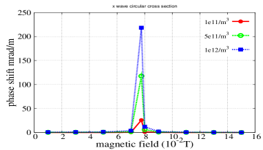
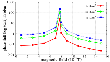
Figure 7: Phase shift vs. magnetic field for dominant X wave propagation for different cloud densities. The peak corresponds to a cyclotron resonance.

Figure [7] shows the enhanced phase shift for three values of cloud densities when the cyclotron frequency approaches the carrier frequency. The beam pipe cross section was circular with a radius of 4.45 cm, which leads to a cutoff at 1.9755GHz at the fundamental $TE_{11}$ mode. These parameters match with the beam pipe geometry of the PEP II/CesrTA chicane section. The wave frequency used in the simulation was 2.17 GHz. The magnetic field corresponding to this cyclotron frequency is 0.077576T. The wave was excited with the help of a sinusoidally varying electric field pointing perpendicular to the external magnetic field.

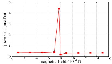
Figure 8: Wave launched with a dominant O wave component showing weak resonance

When the wave is polarized with an electric field that is parallel to the external magnetic field, the mode is often referred to as the Ordinary wave, or the O-wave. In this case one would not expect any effect created by the external magnetic field. This would be the case for a rectangular cross-section waveguide, or with open boundaries. However, with a circular cross section as in our study, the boundary conditions would force a component perpendicular to the magnetic field in the wave electric field even if it is launched with a purely parallel electric field. Thus, it is inevitable that a weak component of a wave with an orthogonal polarization gets excited. Additionally, the method employed in launching the wave in the simulations is similar to that performed in experiments, where an electric field wave is excited along a particular direction over a surface area. The functions describing the wave for a cylindrical geometry are Bessel functions involving the radial and azimuthal variables. Unless care is taken to excite a wave having the given functional form, the wave is expected to couple itself to two orthogonal modes with varying degrees of intensity. Additionally, the detection system, would receive the effect of the two modes to varying degrees. Disentangling this combination will involve more analysis, guided by simulations. Due to these effects, we see a weak resonance effect even in a wave excited with a purely vertical electric field, that is aligned to the external magnetic field as indicated. Figure 8 shows the presence of such a weak resonance and this effect has been observed at CesrTA as well.

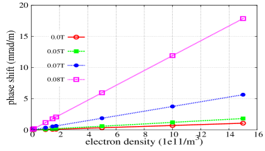
Figure 9: Variation of phase shift with cloud density for different magnetic fields for dominant X-wave propagation.

Figure [9] shows the variation of phase shift with electron cloud density at different settings of external magnetic fields. In these simulations, the wave was excited with an electric field perpendicular to the external magnetic field. These densities are typical of what is produced in CesrTA. The plots show that the variation of phase shift with density remains linear even when one is close to resonance. This is expected to be true as long as the plasma frequency is much smaller than the wave frequency, regardless of how complex the dispersion relationship of the wave is. Thus, one could easily amplify the signal with the help of an external magnetic field to monitor relative changes in cloud density, if not the absolute density.

Experiments have been done to study the phase shift across the damping wigglers at CesrTA. These experiments correspond to various bunch currents and wiggler field settings. The wiggler field setting influences the measurement in more than one way. The wiggler field affects the motion of the electrons, which influences the secondary production of the cloud. The synchrotron radiation flux is determined by the strength of the wiggler field, and this in turn determines the photoemission rate of the cloud. Both these effects determine the density of the cloud. The electron density is not uniform across the length of the wiggler, as shown in Ref [18]. As already shown in this paper, the external magnetic field, by itself, alters the phase shift for a given cloud density. Given that the wiggler field is rather complex, along with a cloud density that is longitudinally nonuniform, simulations become particularly important to fully interpret results from such an experiment. In this paper, we examine just the effects of the nonuniform wiggler field on the phase shift.

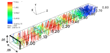
Figure 10: The full Wiggler field in 3 dimensions

The wiggler chamber cross section in CesrTA is close to that of a rectangle. The height is 5cm and width is 9cm. The corners of the rectangle are chopped, so that the actual width of the base and top is 64.6mm and the height of the side walls are 24.6mm. This which would only moderately alter the results obtained from using a perfect rectangle. Thus, for the sake of simplicity, the simulations were done with a perfect rectangle with the above parameters. The length of the section simulated is 80cm, which corresponds to half the length of the wiggler. This is sufficient to account all the variations in the wiggler magnetic field. The computed wiggler magnetic field used was based on the formulation given in [19]. Figure 10 shows the magnetic field, in three dimensions. For most of the region, the field is oriented vertically, while in the transition region between poles there is a longitudinal component to the field. There is almost no magnetic field in the horizontal direction.

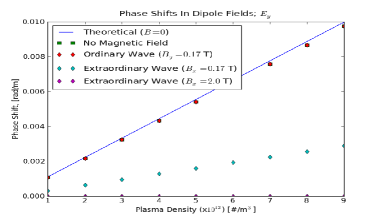
Figure 11: Variation of phase shift with cloud density for different magnetic fields in a rectangular chamber with a vertical wave electric field.

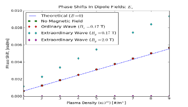
Figure 12: Variation of phase shift with cloud density for different magnetic fields in a rectangular chamber with a horizontal wave electric field.

Even before performing simulations with the full wiggler field turned on, some preliminary studies were done with a just a constant dipole field within the same geometry. Since the shape of the vacuum chamber cross section is rectangular, the the cutoff frequency of the wave is determined by the polarization of the TE wave. If the wave electric field is pointing in the vertical direction, the cutoff frequency is 1.66GHz and if the field is horizontal, the cutoff is 3 GHz. All simulations were done at a frequency 10% above the respective cutoff. Figure 11 shows the phase shift associated with propagation of a vertically polarized wave under different conditions. The figure shows that when the wave electric field is polarized along the external magnetic field, the phase shift matches with that predicted by Eq (1). This result is expected to be true in the case of a rectangular cross section, where the wave electric field is pointing parallel to the external magnetic field everywhere in the pipe, and is thus unaffected by the external magnetic field. As already shown, this would not be true in the case of a curvature in the cross-section boundary. The figure also shows that the phase shift is suppressed in the case of the wave electric field pointing perpendicular to the external field, referred to as extraordinary wave. The cyclotron resonance in this case occurs when the magnetic field is equal to $0.06$T and the field here was set to a much higher value. In general, the wave electric field perturbs the electrons, causing them to oscillate and thereby alter the wave dispersion relation. When the external magnetic field is very high, the electrons tend to get locked against any motion transverse to the magnetic field. Since the wave electric field is perpendicular to the external magnetic field they will encounter electrons that tend to be ”frozen”. As a result the wave will undergo reduced electron cloud induced phase shift at magnetic fields much higher than that causing cyclotron resonance for the specific carrier frequency.

Figure 12 corresponds to a wave with the electric field pointing horizontally. This shows similar features as those in Figure 11. The wave frequency is 3.3GHz and cyclotron resonance occurs at field of 0.11 T, and so the figure shows enhanced phase shift at a magnetic field setting close to this value. Exciting the chamber at this higher frequency could be less efficient due to poorer matching between the various hardware components. In addition, one can expect a mixing of modes to take place at higher frequencies because of the presence of various irregularities in a real beam pipe as opposed to a simulated one. Nevertheless, studying this mode is important because the wiggler magnetic field is mostly pointing in the vertical direction. One could amplify the signal by setting a wiggler field so that a cyclotron resonance is excited. This effect might prove useful in detecting the presence of very low density electrons in wiggler regions. The presence of low energy electrons in wiggler and undulators is of particular interest if the device is cryogenic, in which case the electrons are believed to contribute to the heat load of the system [20]. The electron cloud in such systems would be produced by electron beams primarily through photoemission, and thus if present, they will occur at very low densities, requiring greater sensitivity in the detection.

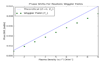
Figure 13: Variation of phase shift with cloud density with the full wiggler magnetic field and a vertical wave electric field.

In the end, we look at the phase shift in the presence of the full wiggler field. Figure 13 shows that the phase shift gets suppressed by about 20% when compared that expected in the absence of any fields. In this case, the wave electric field is pointing in the vertical direction, which is a configuration that should have little effect over the phase shift, since the external magnetic field is largely vertical. A longitudinal magnetic field would alter the dispersion relationship, where the wave gets split into a left and right circularly polarized components. This has been analyzed for guided wave propagation in cylindrical geometries in Ref [11]. While the 20% reduction in phase shift in our result can be attributed to such an effect, a detailed analysis of the same is beyond the scope of this paper. Overall, it is clear that simulations are of prime importance to accurately interpret the observed electron cloud induced phase shifts across such wiggler fields.

5 Summary

In this paper, we provide a comprehensive account of the simulation and analysis effort that has been carried out in conjunction with the experimental effort of using TE waves to measure electron clouds in CesrTA. These simulations helped confirm several physical phenomena either in a quantitative or in a qualitative manner. For example, they helped validate Eq 1 that relates the phase shift with cloud density for geometries like the CesrTA beam pipe, which does not have a regular shape such as rectangular or circular. The effect of reflections on phase shift measurements has always been a concern, and simulations show that one must be careful especially of standing waves excited within the beam pipe due to partial reflectors. The feasibility of using standing waves to measure the cloud density is clearly demonstrated by simulations and has provided valuable guidance to the experimental effort being carried out at CesrTA. In the process, we were able to determine a novel method of detecting the presence of standing waves in simulations by averaging the total Poynting vector flux across a surface over time for varying frequencies.

Simulations of phase shifts in the presence of external magnetic fields were modeled for a variety of cases. The nature of results vary greatly based on the the parameters present in the system. For example, the possibility of exciting cyclotron resonances is clearly shown in simulations, which would be possible to produce in dipole fields present in a chicane. However, dipole fields used in bend regions of an accelerator are much higher and they can suppress the electron induced phase shift, depending on the polarization of the wave. In the presence of curved boundaries, there is always a mixture of effects from ordinary and extraordinary wave propagation. Since most accelerator vacuum chambers have a curvature, this effect is important to understand. A direct comparison with the analytic expression Eq 2 would lead to an incorrect interpretation of the measured data.

The results will always be hard to interpret when a system is near the cyclotron resonance, when the phase shift is theoretically infinity. Simulations and experiments would never yield an infinity, and there may be poor agreement between the two in such regimes. However, an enhancement of the signal that is still predictable can always be obtained by moving reasonably close to a cyclotron resonance point. Electron cloud formation in wiggler fields can be very important in machines such as positron damping rings. Given the complexity of such a system, experiments of determining the cloud density using TE waves have to be accompanied by careful simulations before interpreting any results obtained from measurements.

It may be noted that the relationship between the phase shift and cloud density is always linear regardless of how complex the system is. This would be true for very low cloud densities, which would have low plasma frequencies. Thus, this method can be of great utility if one is interested in relative changes in electron cloud densities for example when a machine is undergoing conditioning. Simulations can then be used to obtain a proportionality constant between cloud density and phase shift.

The studies in this paper were always done with an electron density that was cold and uniformly distributed transversely and longitudinally. Simulations have not indicated a dependence on temperatures associated with typical electron cloud densities. In a transverse nonuniform distribution, there will be a slight enhancement in the phase shift if more electrons are populated in regions with high peak electric fields produced by the wave. As mentioned earlier, longitudinal variation of the cloud density becomes important in wiggler fields because it couples with the longitudinal variation of the magnetic field. These additional complexities could be topics for future studies.

The TE wave method is an attractive technique for measuring electron cloud densities that can replace or complement other measurement methods. Besides CesrTA, this method is being studied at other accelerator facilities [21, 22, 23]. The measurement technique and its required instrumentation are simple, the process is noninvasive, and can be kept in operation continuously. Thus, it holds the promise of wide usage wherever it is useful to monitor the electron cloud properties continuously and at all locations of the accelerator. It is evident that a careful study toward understanding of the physical phenomenon through analysis and simulation are very important toward proper interpretation of the measured data.

6 Appendix: Derivation of Dispersion Relationship

In this Appendix, we provide a derivation of Eq 2 which is not specific to the geometry of the cross-section of the waveguide. We also discuss the approximations and assumptions associated with the derivation of this equation. This dispersion relationship is specific to guided waves propagating through electron clouds in field free regions. The starting equations for such a system would include the fluid and Maxwell’s equations. These are,

$$m[\frac{\partial{\bf v}}{\partial t}+({\bf v}\cdot\nabla){\bf v}]+e({\bf E}+{\bf v}\times{\bf B})=0$$

$$\frac{\partial n_{e}}{\partial t}+\nabla\cdot(n_{e}{\bf v})=0$$

$$\nabla\cdot{\bf E}=\frac{en_{e}}{\epsilon_{0}}$$

$$\nabla\cdot{\bf B}=0$$

$$\nabla\times{\bf E}=-\frac{\partial{\bf B}}{\partial t}$$

$$\nabla\times{\bf B}=\mu_{0}(-en_{e}{\bf v}+{\bf J_{ext}})+\mu_{0}\epsilon_{0}\frac{\partial{\bf E}}{\partial t}$$ (8)

where $n_{e}$ is the number density of the electrons, ${\bf v}$ is the velocity of the fluid, and ${\bf J_{ext}}$ is an external current density. The other terms have their usual meanings. The continuity equation is not independent from the rest of the equations as it can be obtained from Maxwell’s equations.

We perturb all quantities about an equilibrium, so that we have ${\bf v}={\bf v_{0}}+{\bf v^{(1)}}$, $n_{e}=n_{0}+n^{(1)}$, ${\bf E}={\bf E_{0}}+{\bf E^{(1)}}$, ${\bf B}={\bf B_{0}}+{\bf B^{(1)}}$ where the zeroth order quantities satisfy the steady state condition ${\partial}/{\partial t}=0$. As a result, we get

$$m({\bf v_{0}}\cdot\nabla){\bf v_{0}}+e({\bf E_{0}}+{\bf v_{0}}\times{\bf B_{0}})=0$$

$$\nabla\cdot(n_{0}{\bf v_{0}})=0$$

$$\nabla\cdot{\bf E_{0}}=\frac{en_{0}}{\epsilon_{0}}$$

$$\nabla\cdot{\bf B_{0}}=0$$

$$\nabla\times{\bf E_{0}}=0$$

$$\nabla\times{\bf B_{0}}=\mu_{0}(-en_{0}{\bf v_{0}}+{\bf J_{ext}})$$ (9)

Such an equilibrium state requires for the particles to be confined in a steady state indefinitely. This is normally associated with neutral plasmas in which the ions may be considered immobile, or charged particles trapped for a long period of time in confinement devices. In this paper, the electron cloud density is sustained for the duration of the bunch train passage. The above equilibrium condition may be considered valid as long as $1/\tau\gg f$ where $\tau$ is time of confinement of the charge and $f$ is the frequency of the perturbing wave. Periodic changes in the state occurring over time scales greater than the wave periodicity manifest themselves as modulations of the output signal, while changes occurring over much smaller time scales, remain unresolved by the carrier wave. Thus, the spectrum of the output signal would depend on the variation of the electron cloud associated with its build up and decay.

Inserting the perturbation expansion into the original fluid and Maxwell’s equation, and imposing the above equilibrium conditions and ignoring terms of second and higher order, we get,

$$m{\frac{\partial{\bf v^{(1)}}}{\partial t}}+e({\bf E^{(1)}}+{\bf v^{(1)}}\times{\bf B_{0}})=0$$

$$\frac{\partial n^{(1)}}{\partial t}+\nabla\cdot(n_{0}{\bf v^{(1)}})=0$$

$$\nabla\cdot{\bf E^{(1)}}=\frac{en^{(1)}}{\epsilon_{0}}$$

$$\nabla\cdot{\bf B^{(1)}}=0$$

$$\nabla\times{\bf E^{(1)}}=-{\bf\frac{\partial B^{(1)}}{\partial t}}$$

$$\nabla\times{\bf B^{(1)}}=\mu_{0}(-en_{0}{\bf v^{(1)}}+\epsilon_{0}\frac{\partial{\bf E^{(1)}}}{\partial t})$$ (10)

These equations are linear and we can seek all perturbations to have the following form,

$${\bf v}^{(1)}(x,y,z,t)=\tilde{{\bf v}}(x,y)e^{i(k-\omega t)}$$

$$n^{(1)}(x,y,z,t)=\tilde{n}(x,y)e^{i(k-\omega t)}$$

$${\bf E}^{(1)}(x,y,z,t)=\tilde{{\bf E}}(x,y)e^{i(k-\omega t)}$$

$${\bf B}^{(1)}(x,y,z,t)=\tilde{{\bf B}}(x,y)e^{i(k-\omega t)}$$ (11)

From the above, it is clear that

$$\frac{\partial}{\partial z}=ik,~{}~{}~{}~{}~{}~{}~{}\frac{\partial}{\partial t}=-i\omega$$ (12)

This form is valid as long as the geometry along “$z$”, the longitudinal coordinate is uniform and infinite. This is not entirely true when there are partial reflectors. In the case of perfect reflectors, one would obtain discrete values for $k$, representing standing waves. Thus one can expect that the above form to be more accurate when close to a resonance in the presence of partial reflectors. In general, the reflectors would be small enough so that the above form of solutions can be considered a valid approximation.

For the sake of convenience, we drop the accent  $\tilde{}$  and the arguments $(x,y)$ in the functions given in Eq (11). To simplify the analysis, we make two assumptions, (1) The fluid is cold and at rest. So ${\bf v_{0}}=0$, and (2) the density is uniform, which means $n_{0}$ = constant. We further assume that there is no external magnetic field, which means that ${\bf B_{0}}=0$. In the absence of any static external magnetic fields, the only contribution to ${\bf B_{0}}$ would be the magnetic field produced by the beam. Since the beam is highly relativistic, this would be confined along the length of the bunch. It is reasonable to disregard this when the gap between the bunches is much larger than the bunch length, in which case the wave would sample mostly a field free region.

Inserting the waveform solutions (Eq 11) into the perturbed momentum and continuity equations in Eq (10), with ${\bf B_{0}}=0$ and using the relationships of Eq (12), we have,

$$-im\omega{\bf v^{(1)}}+e{\bf E^{(1)}}=0$$

$$-i\omega n^{(1)}+n_{0}\nabla\cdot{\bf v^{(1)}}=0$$ (13)

Combining these, we get

$$n^{(1)}+\frac{n_{0}e}{m\omega^{2}}\nabla\cdot{\bf E^{(1)}}=0.$$ (14)

Combining this with the perturbed electrostatic field equation in Eq (10) gives $n^{(1)}=0$, which means, up to the first order, there is no perturbation in the charge density due to the wave electric and magnetic fields. This gives us

$$\nabla\cdot{\bf E^{(1)}}=0$$ (15)

implying that the wave is purely electromagnetic. By combining the first (momentum), and the last (Ampere’s law) equation of Eq (10), and using the relationships of Eq (12), we get after some algebra,

$$\nabla\times{\bf B^{(1)}}=-i\omega\mu_{0}\epsilon{\bf E^{(1)}}$$ (16)

where $\epsilon=\epsilon_{0}(1-\omega_{p}^{2}/\omega^{2})$. Similarly, it is easy to see that,

$$\nabla\times{\bf E^{(1)}}=i\omega{\bf B^{(1)}}$$ (17)

Using Eqs 15, 16 and 17, along with $\nabla\cdot{\bf B^{(1)}}=0$, and assuming that the boundary conditions are perfectly conducting, one can follow the steps given in Ref[24]. to get

$$\gamma^{2}=\mu_{0}\epsilon\omega^{2}-k^{2}.$$ (18)

The constant $\gamma^{2}$ must be nonnegative for oscillatory solutions, and will take on a set of discrete “eigenvalues”, corresponding to the different modes associated with the geometry of the cross-section of the waveguide. Combining Eq (18) with a similar relationship for a vacuum waveguide where, $\epsilon=\epsilon_{0}$, one can easily show that,

$$k^{2}=\frac{\omega^{2}}{c^{2}}-\frac{\omega_{p}^{2}}{c^{2}}-\frac{\omega_{co}^{2}}{c^{2}}$$ (19)

$\omega_{co}=c\gamma$ being the angular cutoff frequency for the vacuum waveguide. This relationship is the same as Eq (2).

References

- [1] F. Caspers, W. Hofle, J. M. Jimenez, J. F. Malo, J. Tuckmantel, and T. Kroyer, in Proceedings of the 31st ICFA Beam Dynamics Workshop: Electron Cloud Effects (ECLOUD04), Napa, California 2004 (CERN Report No. CERN-2005-001, 2004).
- [2] T. Kroyer , F. Caspers, E. Mahner, Proceedings of 2005 Particle Accelerator Conference, Knoxville, Tennessee 2212-2214
- [3] S. De Santis, J. M. Byrd, F. Caspers, A. Krasnykh, T. Kroyer, M. T. F. Pivi, and K. G. Sonnad Phys. Rev. Lett. 100, 094801 (2008)
- [4] Kiran Sonnad, Miguel Furman, Seth Veitzer, Peter Stoltz and John Cary, Proceedings of PAC07, Albuquerque, New Mexico, USA, pp. THPAS008
- [5] K G Sonnad et al Proceedings of Particle Accelerator Conference 2009, Vancouver, Canada, 2009, pp.TH5RFP044
- [6] J.P. Sikora et al, Proceedings of International Particle Accelerator Conference 2011, San Sebastián, Spain, pp.TUPC170
- [7] K.G. Sonnad et al http://meetings.aps.org/link/BAPS.2007.DPP.TP8.134 49th Annual Meeting of the Division of Plasma Physics
- [8] S. Veitzer, DOE Scientific and Technical Information, http://www.osti.gov/bridge Identifier number 964651
- [9] M. T. F. Pivi, et al, Proceedings of European Particle Accelerator Conference 2008, Genoa, Italy pp. MOPP065
- [10] C. Nieter and J. R. Cary, J. Comp. Phys. 196, 448-472 (2004).
- [11] H. S. Uhm, K. T. Nguyen, R. F. Schneider an d J. R. Smith, Journal of Applied Physics, Vol 64(3), 1988, pages 1108- 1115.
- [12] J. Berenger, Journal of Computational Physics 114, 185 (1994)
- [13] K. Yee, IEEE Transactions on Antennas and Propagation, AP-14, 302 (1966)
- [14] S. De Santis, Phys. Rev. ST Accel. Beams 13, 071002 (2010)
- [15] John Sikora and Stefano DeSantis, http://arxiv.org/abs/1311.5633
- [16] S. De Santis et al, Proceedings of 2011 Particle Accelerator Conference, New York, NY, USA, pp. MOP228
- [17] R J Goldstone and P H Rutherford, Introduction to Plasma Physics Institute of Physics Publishing, 1995
- [18] C. Celata Phys. Rev. ST - Accel. Beams 14, 041003 (2011)
- [19] D. Sagan, J. A. Crittenden, D. Rubin and E. Forest, Proceedings of Particle Accelerator Conference 2003, Portland, OR, USA pp.1023
- [20] S. Casalbuoni, S. Schleede, D. Saez de Jauregui, M. Hagelstein, and P. F. Tavares, Phys. Rev. ST Accel. Beams 13, 073201 (2010)
- [21] S. Federmann, F. Caspers, and E. Mahner, Phys. Rev. ST Accel. Beams 14, 012802 (2011)
- [22] N. Eddy, J. Crisp, I. Kourbanis, K. Seiya, B. Zwaska, S. De Santis Proceedings of Particle Accelerator Conference 2009, Vancouver, BC, Canada pp. WE4GRC02
- [23] J. C. Thangaraj, N. Eddy, B. Zwaska, J. Crisp, I. Kourbanis, K. Seiya Proceedings of the Electron Cloud Workshop 2010, Ithaca, New York, USA pp. DIA00
- [24] J D Jackson. Classical Electrodynamics, Wiley, New York, NY, 3rd ed. edition, (1999)