Sinkless: A Preliminary Study of Stress Propagation in Group Project Social Networks using a Variant of the Abelian Sandpile Model

Abstract

We perform social network analysis on 53 students split over three semesters and 13 groups, using conventional measures like eigenvector centrality, betweeness centrality, and degree centrality, as well as defining a variant of the Abelian Sandpile Model (ASM) with the intention of modeling stress propagation in the college classroom. We correlate the results of these analyses with group project grades received; due to a small or poorly collected dataset, we are unable to conclude that any of these network measures relates to those grades. However, we are successful in using this dataset to define a discrete, recursive, and more generalized variant of the ASM.

Keywords: Abelian Sandpile Model, College Grades, Self-organized Criticality, Sinkless Sandpile Model, Social Network Analysis, Stress Propagation

1 Introduction

At Western Kentucky University, Technical Writing (ENG307) is a required course for students seeking degrees in Professional Writing, Computer Science, Engineering, Management, and so on. Dr. Angela Jones is one instructor of this course; in her sections of ENG307, she assigns a group project where groups of about four students construct some object with “Legos” and compile an instruction manual for how to recreate that object. Front matter of this document would contain a parts list; body matter the instructions; and back matter a notes section. Groups are graded based on the best practices implemented in the manual, a presentation defending their choices, and orderly, timely submission of all project materials.

Included in these project materials are project logs, in which students are asked to record what they did, when they did it, how long was spent doing it, and whether the task was completed individually or collaboratively. Dr. Jones uses these logs to determine whether a student did not sufficiently contribute to the groupwork.

Interested in the effects of social network structure and location on college grades, we saw potential in the contents of these logs. As a preliminary work defining our models and methods, we received from Dr. Jones anonymous PDF scans of project logs for the past three semesters, fall 2012 to spring 2013. In all, there were 53 logs.

To anonymize the logs, all names were replaced with unique identifiers (UID), such as “F3.” The first character of these UIDs represents the group to which the student belonged; the second character serves as an in-group identifier.

In addition to the PDFs, we received a spreadsheet associating with each UID a semester, a grade, a gender, a major, and a year in college, such as freshman and senior.

Groups were assigned by Dr. Jones randomly, adjustments being made if she suspected two or more students would be unable to work together.

2 Related Work

Sparrowe et al apply social network analysis (SNA) to 190 employees spanning five firms in [10]. They distinguish between positive and negative networks, or social networks where nodes are connected by positive and negative relations respectively. In particular, they analyze advice networks (positive) and hindrance networks (negative). Connections for these networks were determined by survey questions, such as “Do you go to [name] for help” or “Does [name] make it difficult.” Performance was measured by surveys answered by group leaders from each of 38 work groups. Sparrowe et al distinguish between individual-level performance and group-level performance, finding distinct correlations for each.

They find that central members in advice networks are rated higher than others; conversely, those central in hindrance networks are rated lower; and paradoxically, highly central groups within a firm are rated lower. Conclusions were based on in-degree centrality, network density, and network centralization measures.

Preparing to perform a similar analysis for our dataset on group projects, we come across the abelian sandpile model (ASM) in the work of D’Agostino et al [4], where it has been adapted for research on financial distress propagation.

Bak et al define the ASM in [1]. Given an infinite 2-dimensional grid, assume “grains of sand” have been dropped thereonto. The amount of sand at a location $(x,y)$ being denoted by $z(x,y)$ and given a critical value $K$, we update each cell of the grid simultaneously according to equation 1. At least one node must be reachable by a path extending from each other node and have $K=\infty$; such nodes are said to be “sinks” because sand “drains out” through them.

$$\begin{split}z(x,y)\rightarrow z(x,y)-4,\\ z(x\pm 1,y)\rightarrow z(x\pm 1,y)+1,\\ z(x,y\pm 1)\rightarrow z(x,y\pm 1)+1,\\ \text{if }z(x,y)>K.\end{split}$$ (1)

Performing a simulation on this model involves initializing the grid with a random distribution of sand, allowing the sand to propagate according to equation 1 until the cascade halts, and probing the system by sequentially dropping additional grains of sand.

To apply this model to financial distress, D’Agostino et al adapt it to operate on networks of any structure: when a node has received an amount of sand exceeding its threshold, it “topples,” donating one of its grains to each of its neighbors. Next, they let sinks represent banks under the coverage of a central bank; that is, these banks are “immunized” against bankruptcy.

They construct scale-free networks, or informally those produced by a “rich get richer” effect. Analyzing the frequencies of cascades of various sizes, they conclude that networks whose degree-degree correlation is positive are more likely to experience a pandemic, yet the speed of pandemic diffusion is decreased.

Others have made similar adaptations of the ASM, including applications in modeling blackouts [3], data-packet transportation [8], rivers [9], and superconductors [7].

In this paper, in section 3.2 particularly, we define a variant of the ASM that achieves self-organized critical behaviors without the requirement for sinks.

3 Experimental Models

3.1 Friend Approximation Network

Because the project logs were hand-written by students and inconsistently filled out, we were unable to use these to define a social network. Turning to the spreadsheet filled out by Dr. Jones, we assume for the sake of this preliminary work that two students are friends if they either (1) are in the same group or (2) share the same college year and major; students may only be connected if they are in the same Technical Writing class. These assumptions are based on intuition that students who share majors and years are more likely to have other classes together and that students who communicate often are more likely to be friends.

We define our social network, denoted by an adjaceny matrix $G$, in equation 2.

$$G_{ij}=\begin{cases}1,&\text{GROUP(i)=GROUP(j)}\\ 1,&\text{MAJOR(i)=MAJOR(j)}\wedge\text{YEAR(i)=YEAR(j)}\\ 0,&\text{Otherwise}\end{cases}$$ (2)

We refer to $G$ as a “friend approximation network” (FAN) and say that two students, $i$ and $j$ are “approximately friends” iff $G_{ij}=1$; approximate friendship is undirected, reflected here by $G_{ij}=G_{ji}$.

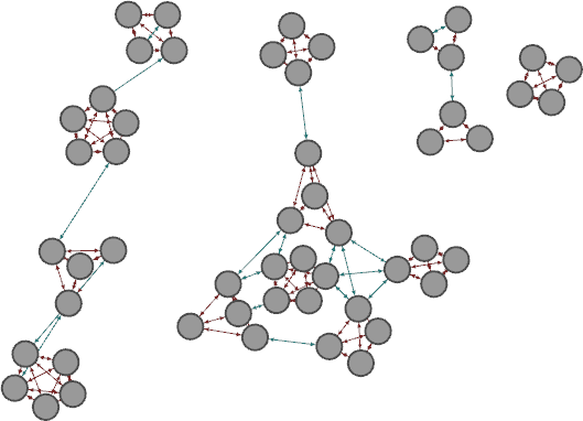
Figure 1: The FAN, containing 53 nodes and 202 edges. Groups form complete subgraphs and are loosely connected to other groups. The leftmost subgraph represents the FAN for fall 2012, the center for spring 2012, and the rightmost two for spring 2013.

3.2 Sinkless Sandpile Model

Because students cannot support an unlimited amount of stress and because we wish not to introduce additional nodes that can, we remove sinks from our sandpile model. So to prevent infinite loops from occuring, we allow nodes to “blow away” a fraction of a grain of sand each time they would topple. Before a node $i$ topples, the sand at $i$ is decreased by some parameter $0<g<1$. Interestingly, if $g=1$, our model is equivalent to an ASM with a sink connected directly to each node.

We denote the network-level carrying capacity (CC), or maximum amount of sand holdable before a topple must occur, as $K$. We denote the CC for node $i$ as $k_{i}$; that is, $k$ is a vector of node-level CCs.

To determine $K$ and $k$, we can either assign all $k_{i}$ values and sum them to receive $K$ or assign $K$ and distribute that sum over all $k_{i}$ values. We find that the second option allows easier comparison of results from networks of different size and structure.

We define $k_{i}$ at first based on a share of $K$ proportionate to node $i$’s degree. Equation 3a shows this basic definition, where $DEG(i)$ is the number of neighbors of $i$.

To generalize further, we introduce a parameter $P$ into that equation, producing equation 3b. When $P=1$, the CC distribution is relative to the degree distribution of the network; when $P=0$, CCs are equally distributed; when $P>1$ or $P<0$, the CC is disproportionately distributed relative to degree distribution, where $P>1$ intensifies the relationship and $P<0$ inverses it.

$$k_{i}=K\frac{DEG(i)}{\sum_{j}DEG(j)}$$ (3a)

$$k_{i}=K\frac{DEG(i)^{P}}{\sum_{j}\left(DEG(j)^{P}\right)}$$ (3b)

$$K\geq(min(DEG)+g)*\sum_{j}(DEG(j)^{P})\div\begin{cases}min(DEG)&P\geq 0\\ max(DEG)&P<0\end{cases}$$ (3c)

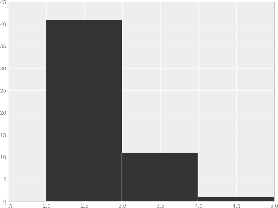
(a)

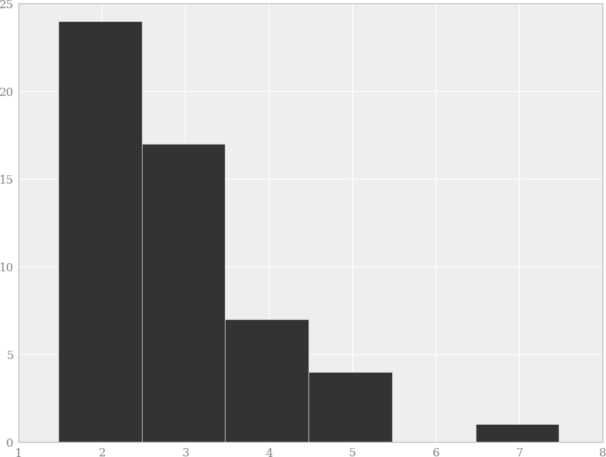
(b)

Figure 2: CC distribution for the friend approximation network when $P=1$ (left) and $P=2$ (right)

We require that $k_{i}\geq DEG(i)+g$ for all $i$ in order to prevent a topple from reducing the amount of sand at any node to a negative value. The minimum acceptable $K$ follows from equation 3c.

We denote the number of grains to drop in the simulation as $X$. In order to provide enough time for the model to reach self-organized criticality [1], we require $X\gg K$.

We denote the amount of sand at node $i$ and time $t$ as $S(i,t)$. We denote the neighbors of $i$ as $N(i)$. We denote the nodes toppling at time $t$ as $T(t)$ and define it in equation 4a. We denote the toppling neighbors of $i$ at time $t$ as $TN(i,t)$ and define it in equation 4b.

$$T(t)=\left\{i|S(i,t)>k_{i}\right\}$$ (4a)

$$TN(i,t)=N(i)\cap T(t)$$ (4b)

We denote a random sequence of integers inclusively between $1$ and the number of nodes as $RND$. So that grains are not dropped during a cascade, we define $ZRND$ in equation 5a.

Our model may then be defined by the recurrence relation in equation 5b.

$$ZRND_{t}=\begin{cases}RND_{t}&T(t)=\emptyset\\ 0&\text{Otherwise}\end{cases}$$ (5a)

$$\begin{split}S(i,t+1)=S(i,t)+|TN(i,t)|\\ +\begin{cases}1&ZRND_{t}=i\\ 0&\text{Otherwise}\end{cases}-\begin{cases}DEG(i)+g&i\in T(t)\\ 0&\text{Otherwise}\end{cases}\end{split}$$ (5b)

We “halt” $S(i,t)$ at the earliest $t$ where the first $t$ elements of $ZRND$ contain $X$ nonzero values.

Summarizing informally, we drop $X$ grains of sand sequentially onto the network. When a node has received an amount of sand greater than its CC, it topples. When a node topples, its amount of sand is first decreased by $g$ and then, for each neighbor of that node, a single grain is taken from it and given to that neighbor. If multiple nodes would topple at once, their amounts of sand are updated synchronously.

A python implementation of this process is given in Appendix A.

4 Experimental Results

We performed 1,000 simulations each for 20 different configurations of the above model, with $X=2500$, $g=0.1$, $K=880$, $P\in[-2..2]$, and $G$ representing any of the three semesters or all three combined. In all, 50,000,000 virtual grains of sand were dropped. We recorded the number of topples that occured for each node during each simulation and the network-total number of topples (NTNT) that occured after each grain of sand during each simulation.

Nearly identical patterns emerged in all 20,000 simulations; in particular, the average rate of growth of NTNT for each configuration of parameters converged to the same linear trend after about 2,300 grains were dropped and propagated. The observed NTNT for any single simulation behaved unpredictibly, albeit following this linear trend. Before the critical point of 2,300 grains, each configuration behaved uniquely; each simulation for a given configuration tended towards the same behavior regardless of how many grains had been dropped.

Figure 3 provides a few examples.

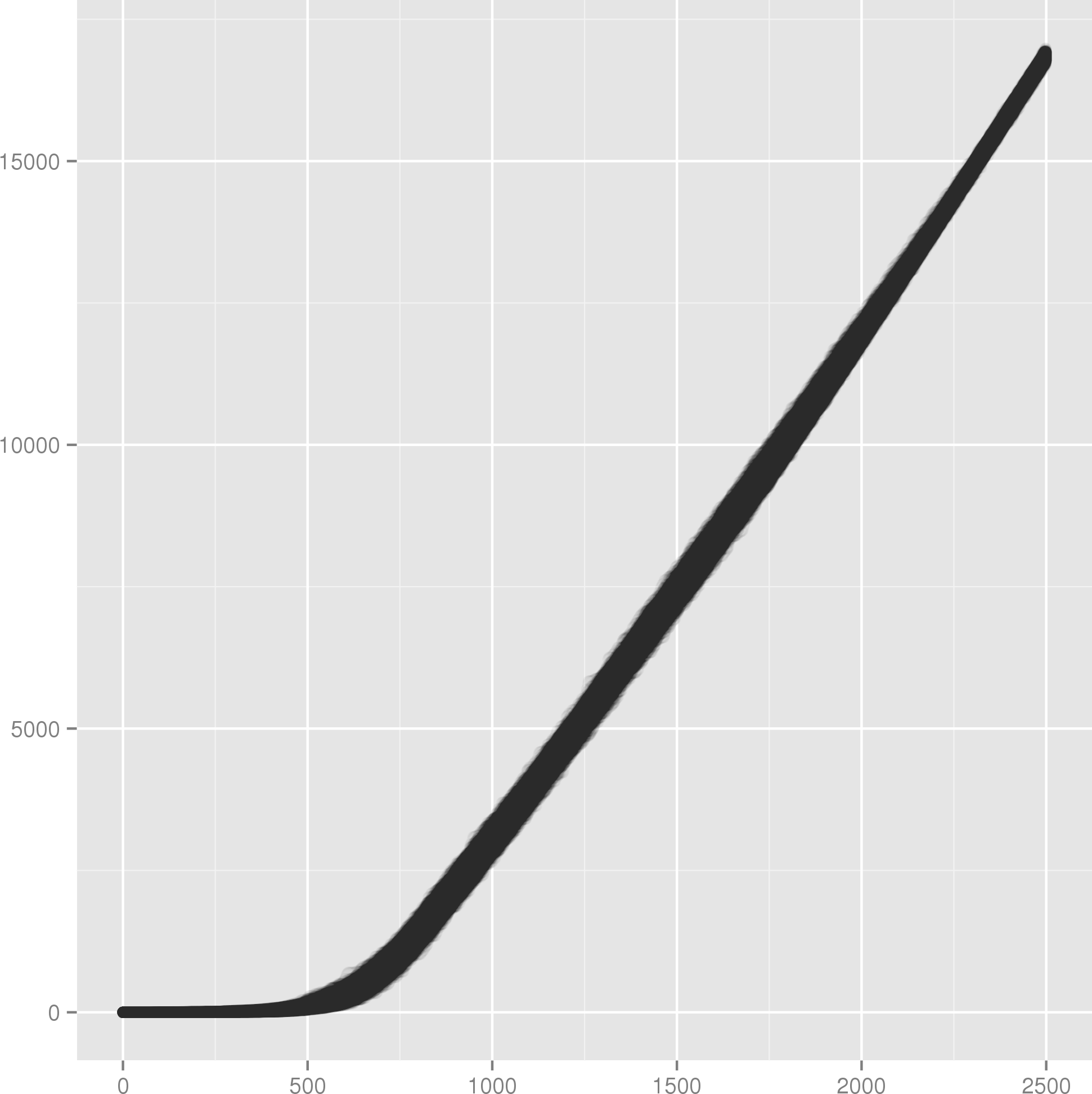
(a)

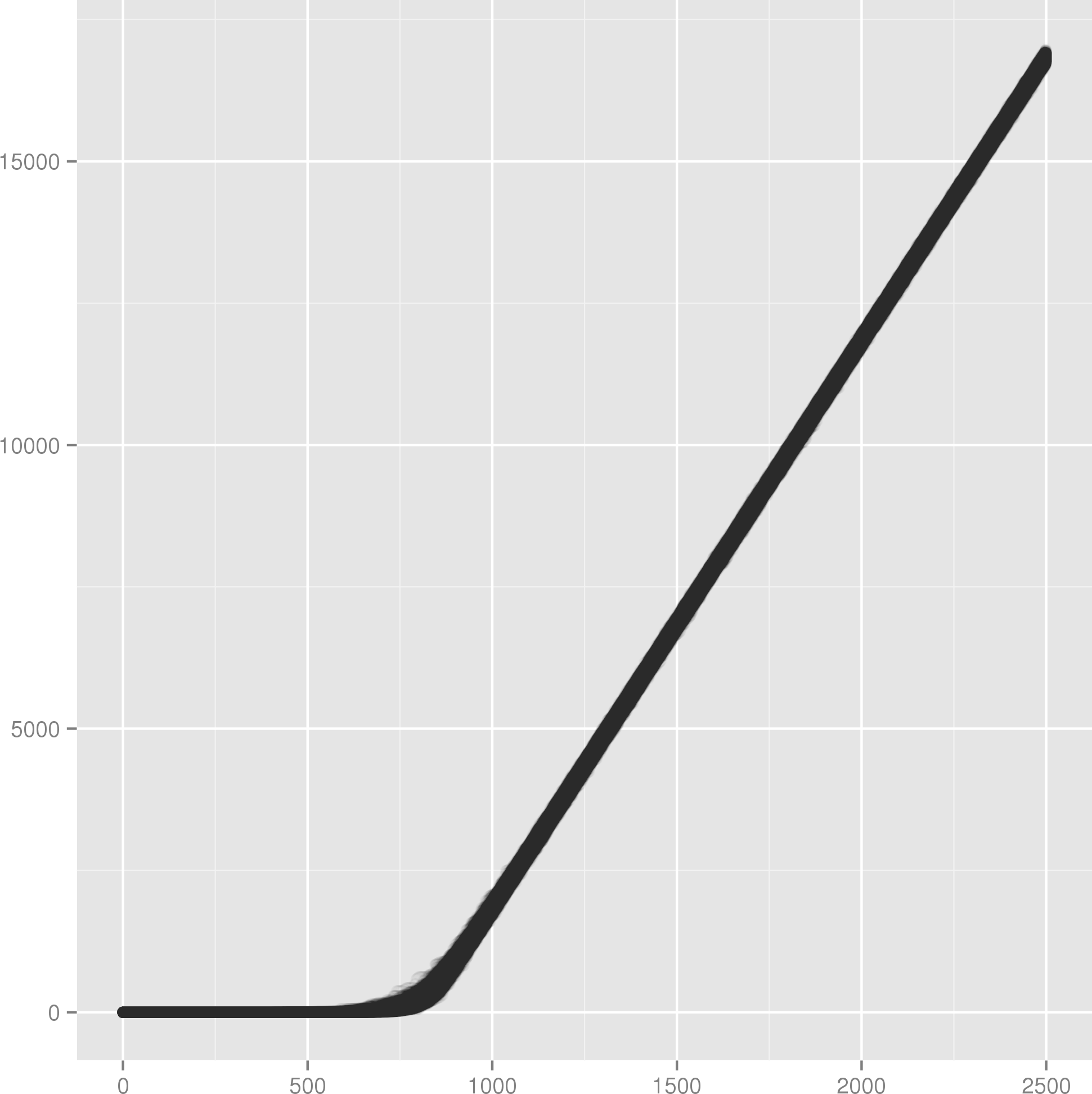
(b)

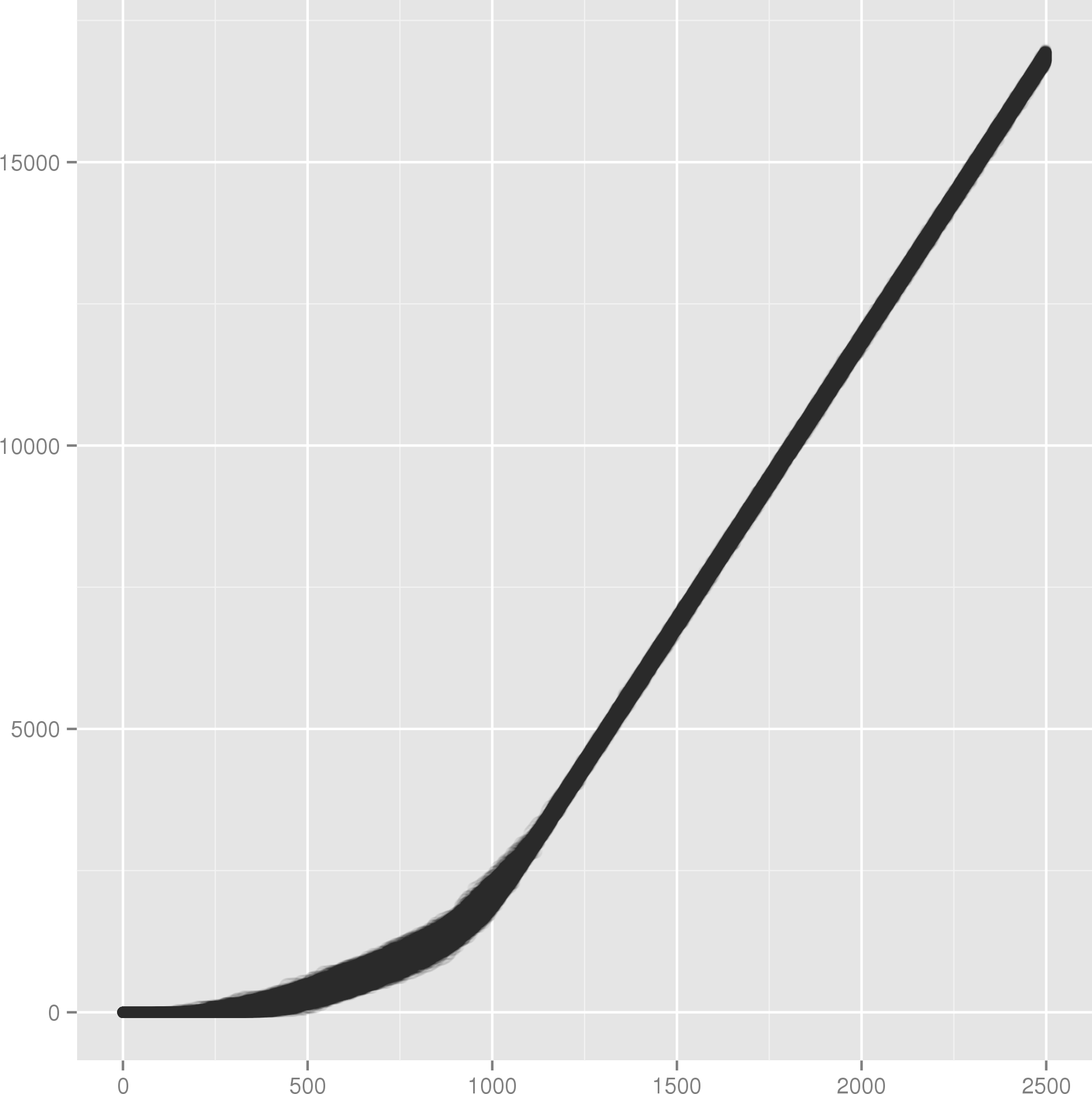
(c)

Figure 3: NTNT growth for full dataset where $P=-2$ (left), $P=0$ (middle), and $P=2$ (right). Points are plotted for all 1,000 simulations at 1% opacity each.

Plotting topples occured against grades received, we notice a few weak trends. When $P=0$, students that recieved As, Bs, and Cs all averaged close to the same number of topples, regardless of other parameters.

When $P=1$ in the fall 2012 network, Bs experienced the most topples and Cs were a close third; in the spring 2012 network, Bs still experienced the most, but Cs were in second and the deviation between the three letter grade groups was small; in the spring 2013 network, Bs experienced far fewer topples than either As or Cs, who were almost identical; and in the full network, results were similar to that of the spring 2012 network with less deviation between the three letter grade groups. We note that the spring 2012 network was the largest and made up roughly 47% of the full network.

When $P<0$, the order of the results were the reverse of those of when $P>0$. When $|P|$ increases, the deviation between the number of topples received increases between the three letter grade groups.

Figure 4 shows the results for one configuration. Note the grouping of grades into three distinct groups, corresponding to As, Bs, and Cs. This is an effect of Dr. Jones’s grading procedure on projects: roughly, she first determines whether the submission is A-work, B-work, or C-work; next, she assigns a numerical grade producing that letter grade; finally, she adjusts based on details like spelling and whitespace management.

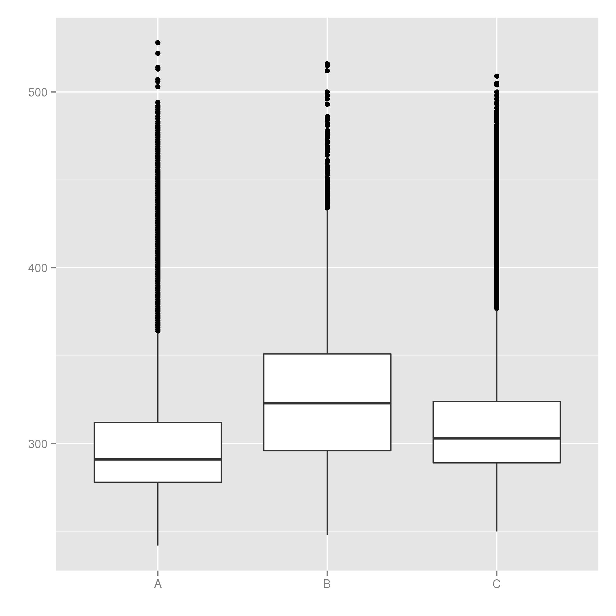
(a)

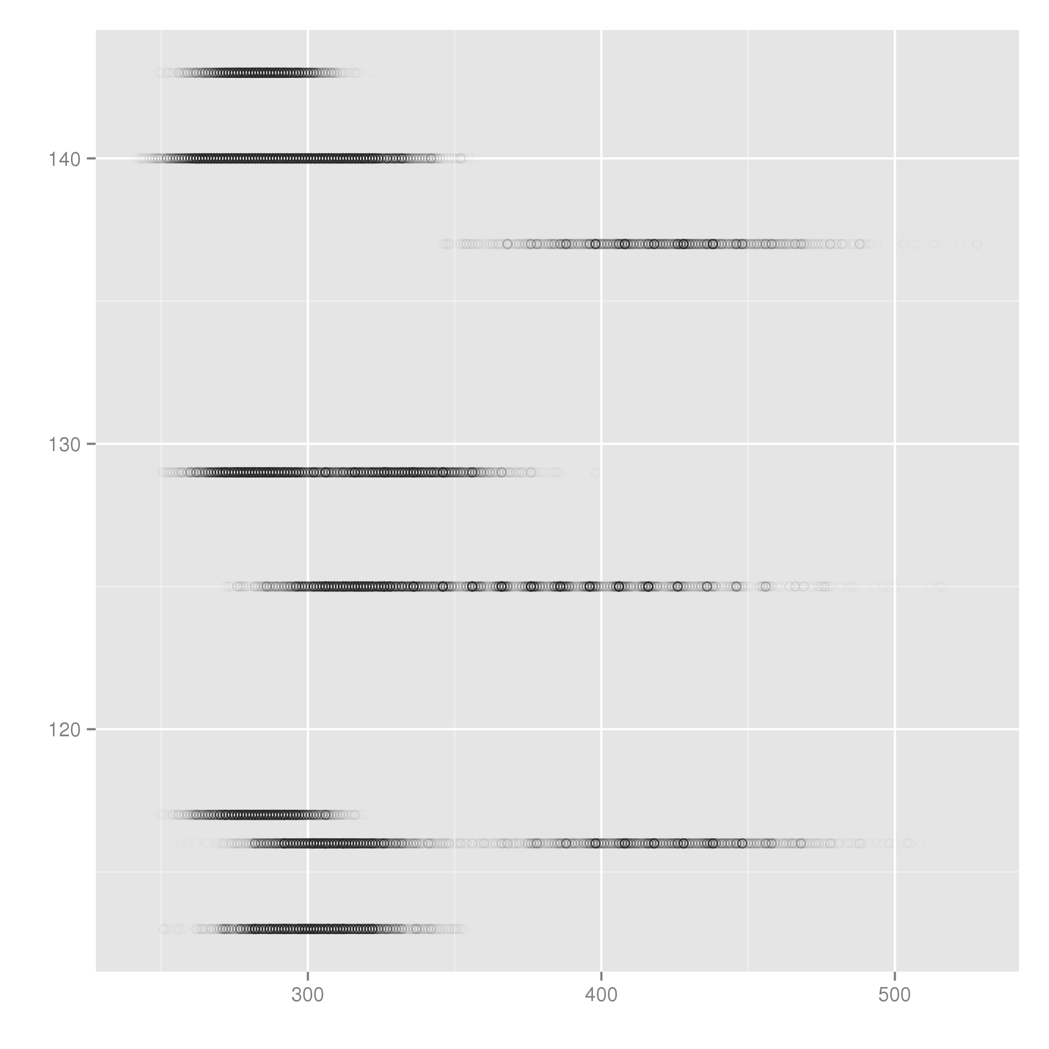
(b)

Figure 4: Plots for topples occured against grades received for the full network, $P=2$, and all 1,000 simulations. Points on the right are plotted at 1% opacity each.

5 Comparisons

The results from our simulations were weak, so to compare out method’s performance with that of common SNA measures, we calcualte Pearson correlation cofficients of grades vs. measure values for seven metrics in additional to our own.

We, like [10], divide these into two levels: member- and group-level. Member-level measures included topples occured and eigenvector, degree, and betweeness centrality, as defined in [5, 6, 2]. Group-level measures included average intergrade, average year, gender ratio, and size. Because of the relatively fixed group size of about four members, the last two of these were uninteresting.

Although the project logs were unusable in constructing a social network, they contained information providing additional insights. Students were asked to grade one another in their groups. To avoid confusion with individual or group grades, we refer to these as “intergrades.” The average intergrade for a group then is the mean of the intergrades assigned to its members by its members.

The average year of a group is simply the mean of values assigned to its members based on college year: freshmen recieved $1$s, sophomores received $2$s, and so on.

All eight of these measures produced correlations weaker than $\pm.3776$. They are summarized in table 1.

Member-level		Group-level
Metric	$\rho$	Metric	$\rho$
Topples	$-.1930$	AvgIntergrade	$+.3073$
Eigenvector	$+.3776$	AvgYear	$+.2278$
Degree	$+.2187$	Gender	$-.1712$
Betweeness	$+.1926$	Size	$+.1392$

Table 1: Pearson correlation coefficients for each of eight metrics against grades received. Full network data was used.

6 Conclusions

We are unable to report a correlation between stress propagation as modeled by our variant of the ASM; further, we are unable to report correlations between SNA metrics that have received considerable and growing attention in the field [2].

Because these SNA measures have been found to correlate strongly with performance in other data, both positively and negatively depending on the given network [10], we believe that our failure in finding a correlation among these methods suggests either the dataset is too small, the collection methods were flawed, our friend approximation network was based on unsound assumptions, or some combination thereof.

We were aware of these issues early on; however, obtaining rigorous datasets on student grades is nontrivial given concerns of privacy and the 1974 act, FERPA. Instead for this preliminary work, we have taken our time to define and explore a novel adaptation of a “sinkless” sandpile model. We define it using recurrence relations and discrete timesteps, allowing it to be easily further adapted for deterministic applications. Additionally, the ASM is reducible to our model by assigning $g=0$ and at least one $k_{i}=\infty$. Alternate strategies of determining $k$ may be implemented by making changes to equation 3b; doing so requires care to ensure $k_{i}\geq DEG(i)+g$ for all nodes $i$.

Beyond our interests in student grades, then, we hope to provide a more general model of self-organized criticality to the field [1].

7 Special Thanks

We would like to thank Western Kentucky University for supporting this work through a Faculty/Undergraduate Student Engagement (FUSE) grant; Dr. Jones for her hard work anonymizing and digitizing student logs, as well as preparing the spreadsheet that made this project possible; and Benjamin Thornberry for his always helpful assistance and feedback.

Appendix A: Python Implementation

⬇

def simulation(G, X, g, k):

# initialization

N = len(G)

S = [0.0 for i in range(N)]

T = [0 for i in range(N)]

deg = [sum(G[i]) for i in range(N)]

# drop X grains sequentially

for x in range(X):

i = randint(0, N-1)

S[i] += 1

# if i topples, assume a cascade

if S[i] > k[i]:

# until cascade stops…

while True:

# find topplers

A = [j for j in range(N) if S[j] > k[j]]

if len(A) == 0:

break

else:

# find how to move sand

B = []

for j in A:

T[j] += 1 # tally topple

S[j] -= g # blow away

S[j] -= deg[j]

C = [m for m in range(N) if G[j][m]==1]

B.extend(C)

# move sand

for b in B:

S[b] += 1

return T

References

- [1] Per Bak, Chao Tang, and Kurt Wiesenfeld. Self-organized criticality: An explanation of 1/f noise. Phys. Rev. Lett., 59:381–384, 1987.
- [2] Stephen Borgatti. Centrality and network flow. Social Networks, 27:55–71, 2005.
- [3] B. Carreras, V. Lynch, M. Sachtjen, I. Dobson, and D. Newman. Modeling blackout dynamics in power transmission networks with simple structure. In Hawaii International Conference on System Sciences. IEEE, 2001.
- [4] G. D’Agostino, A. Scala, V. Zlatic, and G. Caldarelli. Robustness and assortativity for diffusion-like processes in scale-free networks. EPL, 97, 2012.
- [5] Reinhard Diestel. Graph Theory. Springer-Verlag, 3rd edition, 2005.
- [6] Linton Freeman. A set of measures of centrality based upon betweenness. Sociometry, 40:35–41, 1977.
- [7] S. Ginzburg and N. Savitskaya. Self-organization of the critical state in granular superconductors. Journal of Experimental and Theoretical Physics, 90:202–216, 2000.
- [8] E. Lee, K. Goh, B. Kahng, and D. Kim. Robustness of the avalanche dynamics in data-packet transport on scale-free networks. Phys. Rev. E, 71, 2005.
- [9] L. Prigozhin. Sandpiles and river networks: Extended systems with nonlocal interactions. Phys. Rev. E, 49, 1994.
- [10] Raymond Sparrowe, Robert Liden, Sandy Wayne, and Maria Kraimer. Social networks and the performance of individuals and groups. Academy of Management, 44:316–325, 2001.