Magnetoresistance of composites based on graphitic disks and cones

Abstract

We have studied the magnetotransport of conical and disk-shaped nanocarbon particles in magnetic fields $\left|B\right|\leq 9\>\mathrm{T}$ at temperatures $2\leq T\leq 300\>\mathrm{K}$ to characterize electron scattering in a three dimensional disordered material of multilayered quasi 2D and 3D carbon nanoparticles. The microstructure of the particles was modified by graphitization at temperatures $1600^{\circ}\mathrm{C}$ and $2700^{\circ}\mathrm{C}$. We find clear correlations between the microstructure as seen in transmission electron microscopy and the magnetotransport properties of the particles. The magnetoresistance measurements showed a metallic nature of samples and positive magnetoconductance which is a signature of weak localization in disordered systems. We find that the magnetoconductance at low temperatures resembles quantum transport in single-layer graphene despite the fact that the samples are macroscopic and three dimensional, consisting of stacked and layered particles, which are randomly oriented in the bulk sample. This graphene-like behaviour is attributed to the very weak interlayer coupling between the graphene layers.

1 Introduction

The electronic properties of the carbon allotropes, such as nanotubes, graphene [1, 2, 3] and graphite [4] are controlled by the object dimensionality [5], microscopic structure, disorder [5, 6, 7], charge carrier type, density of carriers and their mobility [1, 2, 3], temperature and external electric or magnetic fields [1, 2, 3, 8, 9, 10].

Electronic transport in conventional 2D systems structures or thin films with magnetic impurities was explained by Hikami et al.[11]. For 3D systems this theory was extended by Kawabata [12].

Recent studies of graphene-like materials such as bi-layer graphene and modified multi-layer graphene [13, 14, 15, 16] have shown both weak localization and weak antilocalization phenomena depending on the sample preparation. The differences may partly be attributed to variations in the stacking of the graphene layers from the normal AB or Bernal type toward twisted commensurate layers which was reported [16] to enhance interlayers couplings and scattering. Theoretical modeling [17] has shown that twisting of bilayer graphene, e.g., by twist angle $\theta=21.8^{\circ}$, can give commensurate structures and strongly modified interlayer coupling. Producing bilayer or multilayer graphene with controlled twist angles is an extremely challenging task. However, there may exist naturally occurring multilayered graphene or pyrolytic graphite-like materials that can resemble such configurations. Possible candidates that may contain twisted graphene are the carbon cone particles [18]. These are conical or disk-shaped graphitic-like particles, and it has been reported that certain of these show edge faceting which might be consistent with an alternating twist angle of about $22^{\circ}$ between adjacent layers [19]. Our motivation for the current study was to see how this conical topology influences the electronic scattering mechanisms as may be recorded in magnetoresistivity. We investigate resistance versus temperature and conductance versus magnetic field of a powder of nanoparticles that was bound into mm-sized samples using polymer binder. The nanocarbon particles were mainly cone- and disk-shaped and were prepared with varying degree of graphitization. These nanocarbon-polymer composite samples are apparently similar to granular conductors [20, 21].

The conductance versus magnetic field of the heat treated (HT) samples displayed features of 2D transport. We find that the magnetoconductivity model developed in the theory of McCann et al. [22] for 2D graphene is suitable for discussing our experimental data at low temperatures [23]. We can partially explain the observed behaviour as effect of very weak coupling between misoriented layers [15, 24, 25] inside the disks and cones.

2 Sample descriptions

2.1 Nanocarbon particles

The graphitic-like carbon powder was produced by the so called “Kvaerner Carbon Black and Hydrogen Process” [26] which is an industrial, pyrolytic process that decomposes hydrocarbons into hydrogen and carbon using a plasma torch at temperatures above $2000^{\circ}\>\mathrm{C}$. The as produced, ”raw” powder (in the following denoted HT-0) consists of flat nanocarbon disks, open-ended carbon cones, and a small amount of carbon black-like structures as seen in electron microscopy images [18, 19, 27, 28]. In order to improve the crystalline quality of the particles, additional heat treatment was done at high temperatures in an argon atmosphere for three hours, followed by a slow natural cooling. In this study, heat treatment was done at either $1600^{\circ}\>\mathrm{C}$ (HT-1600) and $2700^{\circ}\>\mathrm{C}$ (HT-2700).

The carbon disks and cones exhibit a wide range of diameters ($500-4000\>\mathrm{nm}$) with wall thicknesses of typically $10-30\>\mathrm{nm}$. However, particles with thickness in the range $5-70\>\mathrm{nm}$ can be found. Krishnan et al. [18] showed that the observed macroscopic cone apex angles correspond to those of perfect graphene cones with apex angles $\alpha=112.9^{\circ}$, $83.6^{\circ}$, $60.0^{\circ}$, $38.9^{\circ}$, and $19.2^{\circ}$. Perfect graphene cones are defined by $n=1-5$ pentagonal disclinations incorporated in close proximity in a graphene sheet. Upon extension, the flat disks can be considered as cones with $n=0$, i.e., with no pentagons. Some of the disks and the cones with a $112.9^{\circ}$ apex-angle showed six-fold and five-fold faceting, respectively [29]. Transmission electron microscopy (TEM) selected area diffraction (SAD) patterns of a disc and cones in [19, 29] exhibit concentric continuous rings including as set of distinct spots with six-fold rotational symmetry and were interpreted in terms of discs comprising a highly crystalline graphitic core enveloped by much thicker layer of disordered carbon. The thickness of the crystalline core in the as-produced disks was estimated to be only $10-30\%$ of the total disk thickness [29]. Recent high-resolution TEM (HR-TEM) micrographs [30] clearly show that the outer enveloping layer of the as-produced disks and cones is turbostratic. Upon heat treatment, the graphitic order increases with increased heat treatment temperature. From HR-TEM images [30] and SAD patterns [19, 30] it is clear that at $2700^{\circ}\>\mathrm{C}$, the structure of the cone and disk envelope can be described by partially overlapping extended graphitic domains wherein graphene layers lack a well defined stacking order. In the present work, HR-TEM micrographs were acquired with a Jeol JEM 2010F microscope operated at 200 kV. Figure 1 shows details of the cone structure at the edge cones heat treated at $1600^{\circ}\mathrm{C}$ and $2700^{\circ}\mathrm{C}$. After heat treatment at $1600^{\circ}\>\mathrm{C}$ the enveloping carbon layer remains turbostratic. However, at $2700^{\circ}\>\mathrm{C}$ extended graphitic domains are clearly present, which indicates a polycrystalline rather than a purely turbostratic structure. While the cone envelope shows varying degrees of disorder depending on HT, the overall cone morphology is dictated by the highly crystalline core. In light of the reported conformity of measured cone apex angles to those expected for idealised graphene cones, it follows that the crystalline cores must conform to a $n=1-5$ disclination topology. Thus the entire structure of these particles are to a first approximation referred to as carbon cones, whilst acknowledging that at the nanoscale the cone structure differs somewhat from that expected for a perfect multilayer graphene cone, depending on heat treatment temperature. Note also that these cones are intrinsically different from such structures as the conical graphite crystals reported by Gogotsi et al. [31] and carbon nanohorns [32].

The investigated composite samples show disorder on at least two length scales. On the nanometer scale they are a mixture of crystalline parts, likely containing many dislocations, grain boundaries and other defects, and non-crytalline/amorphous matter. On the micrometer scale the grainy nature of the powder will make different packings of particles and form a solid sample with a locally varying material density.

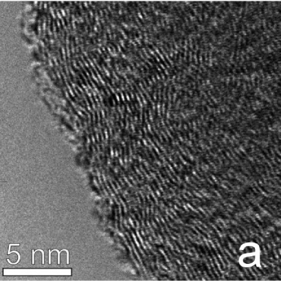
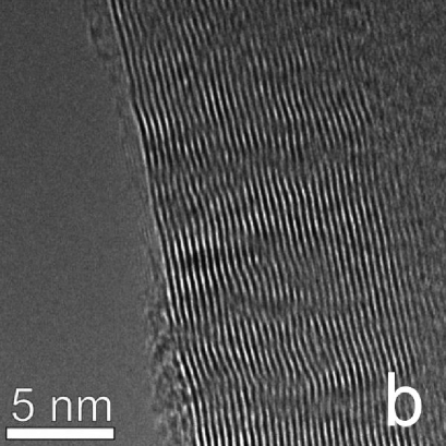
Figure 1: High-resolution transmission electron micrographs showing the microstructure of a) carbon cones raw material and material heat treated at b) $1600^{\circ}\mathrm{C}$, and c) $2700^{\circ}\mathrm{C}$.

The crystallinity of the nanocarbon powder was investigated by powder x-ray diffraction using a Bruker AXS D8 Advance diffractometer with $\mathrm{CuK}_{\alpha}$ ($\lambda=1.5418\>\mathrm{\mathring{A}}$) radiation and a LynxEye detector. The powder was filled in $1.5$ mm glass capillaries. The interlayer distance was found to be $\frac{c}{2}=3.53\pm 0.03\>\mathrm{\mathring{A}}$, $3.464\pm 0.015\>\mathrm{\mathring{A}}$, and $3.373\pm 0.001\>\mathrm{\mathring{A}}$ for the HT-0, HT-1600, and HT-2700 samples, respectively. The typical size of the crystalline domains was estimated from the full-width at half-maximum of the diffraction peaks using the Scherrer equation [33]. The coherence length perpendicular to the graphene layers, $L_{c}$, increased from the range $1-3$ nm for the raw material (HT-0) to $4.5\pm 0.8$ nm and $38\pm 6$ nm for the samples annealed at $1600^{\circ}\mathrm{C}$ and $2700^{\circ}\mathrm{C}$, respectively. This means that in particular the heating to $2700^{\circ}\mathrm{C}$ had a significant influence on the crystalline order, in qualitative agreement with the HR-TEM images in figure 1. Naess et al. [29] reported that the in-plane coherence length $L_{a}\approx 20$ nm for samples similar to our HT-2700 material. These authors also reported a faceting along the edges of the disks and the 5-pentagon cones into pairs of sectors of about 22^∘ and (60-22)^∘= 38^∘, possibly reflecting an underlaying twisted hexagonal structure. Earlier it has been shown that an alternating shift of the graphene in-plane axis of 21.8^∘ between subsequent layers in a conical or helical cone structure may give an optimal graphitic alignment between the layers [34, 35]. It was proposed [29] that similar alternating layer rotations may exist in the particles of the current carbon material.

In a previous study of magnetic properties of raw nanocarbon powder [36], we have determined a residual amount of Fe using the particle-induced x-ray emission method. In the HT-1600 powder, the content of Fe is $<75\>\mu\mathrm{g/g}$. In HT-2700 powder, the content of Fe is lower than the method can detect ($<3\>\mu\mathrm{g/g}$) [36].

2.2 Bulk sample preparation

In order to prepare a dense bulk sample, carbon powder was mixed with polymethyl methacrylate (PMMA) dissolved in chloroform where the volume of nanocarbon filler was $>60$ vol-%. The resulting viscous solution was placed on a mica substrate of thickness $\sim 30\>\mathrm{\mu m}$ having a four wire arrangement for resistivity measurements, figure 2 (a), inset. The polymerization took place at room temperature. Typical size of the polymerized sample was about $6\times 6\times 0.5\>\mathrm{mm}$ (l $\times$w $\times$t), i.e., the samples were macroscopic three dimensional objects. The reproducibility of the sample preparation method was verified by resistance measurements at room temperature for the same four wire arrangement (figure 2 (a), inset) and other samples with the same sample dimensions. Typical sample resistance was in the range $R=1-15\>\Omega$. The volume fraction of carbon powder in the sample was much higher than the percolation threshold [42], i.e., the sample conductance did not depend qualitatively on the fraction of nanoparticles. Thus, the samples were 3D bodies of randomly stacked disks (quasi 2D objects) and cones (3D objects) with a structure similar to granular conductors [20, 21].

3 Resistance measurement

The polymer-bonded nanocarbon samples were placed in the vacuum chamber of a Quantum Design Physical Property Measurement System (PPMS). The standard four wire method shown in the inset of figure 2 (a) was used to measure the resistance. The samples were driven by an ac current of $10\>\mu\mathrm{A}$ in a resistivity measurement mode of the PPMS. Resistance measurements were performed at several temperatures $2\leq T<300\>\mathrm{K}$ in magnetic fields $-9\leq B\leq 9\>\mathrm{T}$ applied perpendicular to the sample surface. We have verified that samples show linear volt-ampere dependence at $T=300\>\mathrm{K}$ for currents $1\leq I\leq 100\>\mu\mathrm{A}$.

4 Experimental results

The experimental results are presented using either the resistance $R$ (section 4.1) or the conductance $G$ (section 4.2) of the nanocarbon-polymer samples. Resistivity $\rho$ of the samples was determined by taking into account their physical dimensions.

4.1 Resistance versus temperature measurements

The temperature dependence of the resistance $R(T)$ of the HT-1600 sample without a magnetic field is shown in figure 2 (a). In the broad temperature interval $2\leq T<300\>\mathrm{K}$ the experimental data in figure 2 (a) are approximated by:

$$R(T)=\frac{R_{0}}{1+\left(\frac{T}{T_{0}}\right)^{\beta}}+R_{r}$$ (1)

where $R_{0}$, $R_{r}$, $T_{0}$, and $\beta$ are parameters [10]. These parameters are presented in table 1. The residual resistance $R_{r}$ had to be included due to a relatively high sample resistance at room temperature [10].

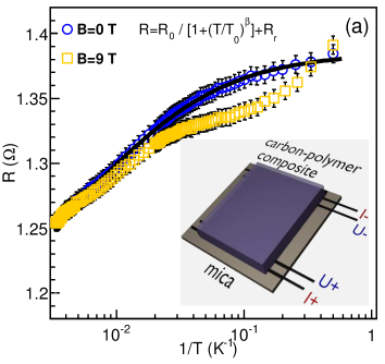
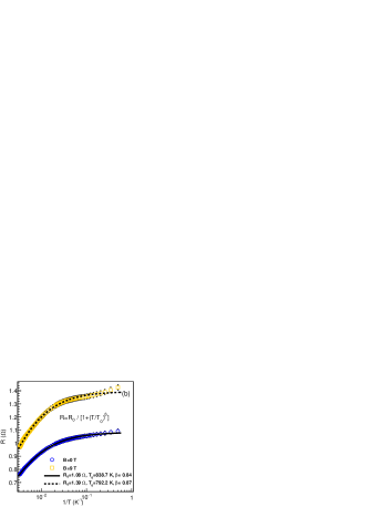
Figure 2: The resistance $R$ versus temperature $T$ for magnetic fields $B=0$ and $9\>\mathrm{T}$. (a) (log-lin plot) polymer sample containing nanocarbon powder heated at $1600^{\circ}\mathrm{C}$ (HT-1600) and (b) (log-lin plot) polymer sample containing powder heated at $2700^{\circ}\mathrm{C}$ (HT-2700). The inset shows the sample design and four-wire geometry used to measure resistance. The fits to the experimental data without magnetic field are shown as solid lines. In (b), the case with applied field $B=9\>\mathrm{T}$, the fit is shown using a dashed line.

In magnetic field $B=9\>\mathrm{T}$, the temperature dependence of the resistance $R(T)$ shows a weak negative MR in the range from room temperature $T\approx 300\>\mathrm{K}$ down to $T\approx 50\>\mathrm{K}$. For lower temperature $10<T<50\>\mathrm{K}$, the negative MR due to the magnetic field is more evident. However at temperature $T\approx 3\mathrm{K}$ the MR changes sign and at temperatures $T<3\>\mathrm{K}$ it is positive.

The temperature dependence of the resistance $R(T)$ of the HT-2700 sample in figure 2(b) may also be approximated by equation (1) but with the residual resistance $R_{r}=0$. The equation approximates experimental data both without and with magnetic field in the broad temperature interval $2\leq T<300\>\mathrm{K}$ (see table 1). In magnetic field $B=9\>\mathrm{T}$, a small deviation from equation (1) was observed for low temperatures $2\leq T<10\>\mathrm{K}$.

Table 1: Parameters extracted in fits of the carbon nanoparticle resistances to equation (1) (HT-1600 and HT-2700 samples).

Sample	$B$ $(T)$	$\beta$	$R_{0}\>(\Omega)$	$T_{0}\>(K)$	$R_{r}\>(\Omega)$
HT-1600	0	0.84	0.19	130.7	1.19
HT-2700	0	0.84	1.08	838.7	0
HT-2700	9	0.87	1.39	792.2	0

The reduced activation energy $W(T)$ may reveal important information about the nature of the transport in the sample, and it is defined as [8, 10]

$$W(T)=-\frac{d\ln\left(\rho\left(T\right)\right)}{d\ln\left(T\right)},$$ (2)

where $\rho(T)$ is the resistivity dependence on temperature $T$. We have determined the reduced activation energies numerically from the experimental data in figure 2 and also analytically from equation 1. The analytical results are: (i) $W(T)=\beta R_{0}z/\left\{\left[R_{r}+R_{0}/(1+z)\right]\left(1+z\right)\right\}$ for the HT-1600 sample, and (ii) $W(T)=\beta z/\left(1+z\right)$ for the HT-2700 sample, where $z=\left(T/T_{0}\right)^{\beta}$. The results of the numerical data analysis (symbols) and analytical expressions (solid lines) are shown in figure 3.

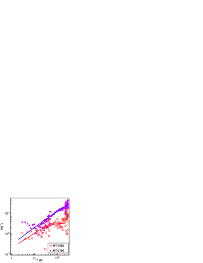
Figure 3: The reduced activation energy $W(T)$ versus temperature $T$ for nanocarbon powders heat treated at $1600$ and $2700^{\circ}\mathrm{C}$. The solid lines are analytical functions calculated for the reduced activation energy $W(T)$.

4.2 Measurements of conductance versus magnetic field

The sample conductance $G(B)$ versus magnetic fields in the range $-9\leq B\leq 9\>\mathrm{T}$ was measured at different temperatures $2\leq T\leq 300\>\mathrm{K}$. We have analyzed the change of conductance $\Delta G=G(B)-G_{0}$ and relative change of conductance $\Delta G/G_{0}$, where the conductance $G_{0}$ is the sample conductance without magnetic field.

We followed the approach by Vavro et al. [10] to scale magetoresistance data using a universal scaling form $Af\left(B/B_{\phi}\right)$. $A$ is the amplitude and $B_{\phi}$ is the magnetic field that induces one magnetic flux quantum $\Phi_{o}$ though a weak localization (WL) electron scattering loop. Here, $\Phi_{0}=h/2e$, with $h$ being Planck’s constant and $e$ the electron charge. We found that a similar universal scaling equation

$$f(cx)=c^{\alpha}f(x),$$ (3)

where $f(x)$ is the relative conductance $\Delta G/G_{0}$, $c$ is a positive constant, and $\alpha$ is a scaling exponent, can be used for our data.

The magnetoconductance of the HT-1600 sample in figure 4 (a) is positive, $\Delta G>0$, at low temperatures $2\leq T\leq 5\>\mathrm{K}$ and low magnetic fields $|B|<6\>\mathrm{T}$. The increase of sample conductance with increasing applied magnetic field is a signature of WL [5]. We found that the graphs of $\Delta G/G_{0}$ versus $B$ for the HT-1600 sample scale into two different curves as displayed in figure 4 (b). Here, the universal scaling equation (3) with the best-fit exponent $\alpha=0.6$ was applied. For temperatures $2\leq T\leq 20\>\mathrm{K}$ one scaling curve was found, and for $50\leq T\leq 100\>\mathrm{K}$ a second curve was obtained.

We have found that the relative change of conductance $\Delta G/G_{0}$ in figure 4 (a) can be approximated by a power law $\Delta G/G_{0}\propto B^{\delta}$, where $0.5<\delta<1$ for temperatures $2\leq T<20\>\mathrm{K}$, $\delta\doteq 1$ for $T=20\>\mathrm{K}$, and $\delta>1$ for $20<T\leq 100\>\mathrm{K}$. For example, in figure 4 (a) for temperature $T=50\>\mathrm{K}$ the exponent $\delta=1.80\pm 0.01$. These values of $\delta$ are different from the expected value $\delta=2$ (see section 5).

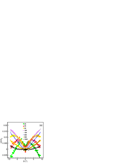
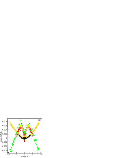
Figure 4: (a) The change of conductance $\triangle G$ versus magnetic field $B$ of carbon powder HT at $1600^{\circ}\mathrm{C}$. The graphs for temperature $T=2,\>3$ and $5\>\mathrm{K}$ are approximated by equation (4) with the fitting parameters presented in table 2. The data for $T=50\>\mathrm{K}$ (dark yellow) are approximated by the equation $\Delta G\propto B{}^{\delta}$ with $\delta=1.80\pm 0.01$, shown as a brown solid line. (b) Using equation (3) the experimental data scale into one single curve for low temperatures $2\leq T\leq 20$. For temperatures $50\leq T\leq 100\>\mathrm{K}$ the same scaling collapsed the data into a second, different curve. The temperature symbols have the same meaning as in (a).

In a similar way, the relative change of conductance $\Delta G/G_{0}$ for the HT-2700 sample, presented in figure 5 (a) could be rescaled in the broad temperature range $2\leq T\leq 300\>\mathrm{K}$. In this case, as seen in figure 2 (b), the effect of the applied magnetic field was much stronger and the maximal relative change of conductance in was about $\Delta G/G_{0}=0.23$. Quite good data collapse using scaling equation (3) was found giving the same exponent as before, $\alpha=0.6$. Here, almost all data scale into the same single curve, figure 5 (b), except data at low temperatures $2\leq T\leq 5\>\mathrm{K}$ and low magnetic fields $\left|B\right|<3\>\mathrm{T}$. The magnetoconductance of this sample shows $\Delta G/G_{0}>0$ for temperatures $2\leq T\leq 20\>\mathrm{K}$ and magnetic fields $\left|B\right|<0.9\>\mathrm{T}$ (figure 6 (b)) which is interpreted as WL.

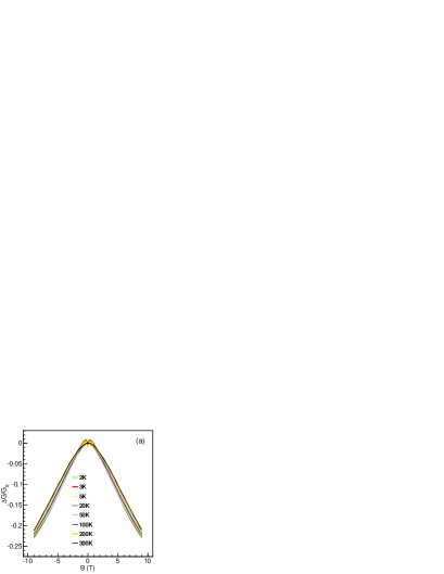
Figure 5: (a) Relative change of conductance $\triangle G/G_{0}$ versus magnetic field $B$ for the HT-2700 sample. (b) The experimental data scale into a single curve except data measured at low temperatures $2\leq T\leq 5\>\mathrm{K}$ and low fields $\left|B\right|<3\mathrm{T}$.

Surprisingly, we have found that the equations developed for the WL in graphene [22] can approximate the data shown in figure 4 and 5. We have fitted our data to the following expression for the relative change of magnetoconductance

$$\Delta G=d\Biggl{[}F\left(\frac{B}{B_{\phi}}\right)-F\left(\frac{B}{B_{\phi}+2B_{i}}\right)-2F\left(\frac{B}{B_{\phi}+B_{i}+B_{*}}\right)\Biggr{]}$$ (4)

where $F\left(z\right)=\ln\left(z\right)+\psi\left(1/z+1/2\right)$, $\psi\left(x\right)$ is the digamma function, $B_{\phi}$, $B_{i}$, and $B_{*}$ are characteristic fields related to the various electron scattering processes in the material, and $d$ is a constant. For graphene [13, 22, 37, 38, 39] the constant $d$ is universal $d=2e^{2}/h$, with $h$ being the Planck’s constant and $e$ the electron charge. It was found that $\tau_{\phi}^{-1}=4DeB_{\phi}/\hbar$ for the inelastic decoherence time $\tau_{\phi}$, where $D$ is the diffusion coefficient, and $\hbar=h/2\pi$. Similar expressions were valid for the intervalley scattering time $\tau_{i}$ and a combined scattering time $\tau_{*}$ [22]. These characteristic times can also be related to characteristic electron scattering lengths given by

$$L_{\phi}=\sqrt{D\tau_{\phi}}=\sqrt{\frac{\hbar}{4eB_{\phi}}},$$ (5)

and similar expressions for the other length scales $L_{i}$ and $L_{*}$ with $B_{i}$ and $B_{*}$, respectively, replacing $B_{\phi}$ in equation (5) [22, 40]. In our case, $d$ in equation (4) is a parameter to approximate the experimental data and is related to the effective number of electron transmission channels [41].

The equation (4) was used to approximate and parametrize the experimental data for the HT-1600 sample in figure 4 (a) and data for the HT-2700 sample shown in figure 6. For low temperatures $T=2,\>3$ and $5\>\mathrm{K}$ we have determined the characteristic $B$-fields, which are presented in tables 2 and 3 for the HT-1600 sample and HT-2700 sample, respectively. For HT-2700 data where fitted only for low magnetic fields $|B|<1\>\mathrm{T}$ except for the $T=2K$ data shown in figure 6 (a) which showed excellent agreement over the whole range of magnetic fields $0.01<B<9\mathrm{\>T}$. The values of the parameter $d$ from equation (4) were determined as $d_{1600}=0.882\pm 0.032\;\mathrm{S}$ and $d_{2700}=0.1558\pm 0.0008\>\mathrm{S}$. The resulting fits are shown as solid lines superimposed on the 2, 3 and 5 K data sets in figures 4 (a), 6 (a) and 6 (b).

Table 2: The characteristic field parameters for the HT-1600 sample at low temperatures calculated from fits to equation (4).

T (K)	$B_{\phi}$ (T)	$B_{i}$ (T)	$B_{\star}$ (T)
2	$1.70\times 10^{-1}$	$6.46\times 10^{-4}$	$21.5$
3	$4.12\times 10^{-1}$	$2.67\times 10^{-3}$	$25.8$
5	$7.83\times 10^{-1}$	$7.40\times 10^{-3}$	$40.7$

According to the results of table 2 and equation (5), the characteristic scattering lengths for HT-1600 are in the ranges $14<L_{\phi}<31\>\mathrm{nm}$, $148<L_{i}<504\>\mathrm{nm}$, and $L_{*}=2.4\pm 0.4\>\mathrm{nm}$. Similarly, for the HT-2700 sample the values calculated from table 3 are in the ranges $66<L_{\phi}<92\>\mathrm{nm}$, $398<L_{i}<603\>\mathrm{nm}$, and $L_{\ast}=13.05\pm 0.15\>\mathrm{nm}$ These values of $L_{\phi,i,*}$ are presented in figure 7 (a).

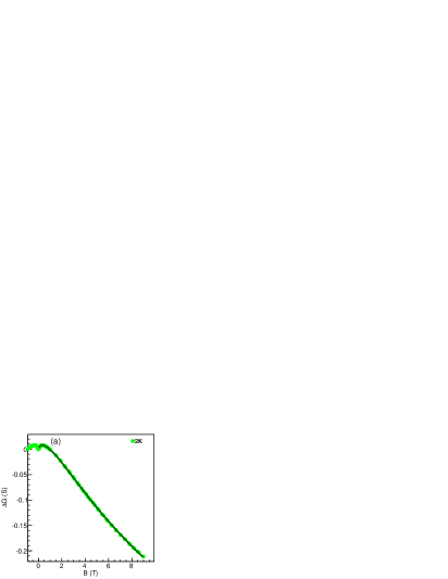
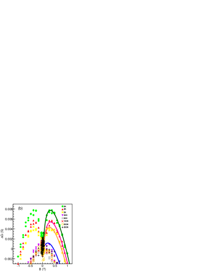
Figure 6: (a) The change of conductance $\Delta G$ versus magnetic field $B$ at $T=2\>\mathrm{K}$ where the experimental data are approximated by equation (4) (dark green, solid line). The fitting parameters are shown in table 3. (b) Weak localization and antilocalization at low temperatures $2\leq T<20\>\mathrm{K}$ and antilocalization at temperatures $T>20\>\mathrm{K}$ at low fields for the sample containing carbon powder HT-2700. The graphs for temperatures $T=2,\>3,\>5$ and $20\>\mathrm{K}$ are approximated by equation (4). The parameters are shown in table 3.

Table 3: The characteristic fields for HT-2700 sample at low temperatures calculated from fits to equation (4).

T (K)	$B_{\phi}$ (T)	$B_{i}$ (T)	$B_{\star}$ (T)
2	$1.98\times 10^{-2}$	$8.17\times 10^{-4}$	$0.94$
3	$2.97\times 10^{-2}$	$1.03\times 10^{-3}$	$0.95$
5	$2.46\times 10^{-2}$	$6.45\times 10^{-4}$	$0.99$
20	$3.71\times 10^{-2}$	$4.53\times 10^{-4}$	$0.95$

From the scaling equation (3) we can determine the parameter $c=1/B_{\phi}$ that collapses the experimental data in figures 4(b) and 5(b). According to equation (5) $B_{\phi}\propto L_{\phi}^{-2}$, and we then find $L_{\phi}^{2}$ from the relation $L_{\phi}^{2}/L_{0}^{2}=B_{0}/B_{\phi}$, where $L_{0}$ and $B_{0}$ are undetermined normalization constants. As before, $B_{\phi}$ is the field related to the effect of one magnetic flux quantum $\Phi_{0}$ and $L_{\phi}$ is the corresponding phase coherence length. The resultant values for the square of the normalized phase coherent length $L_{\phi}^{2}/L_{0}^{2}$ versus $T$ for both samples based on the data scaling are shown in figure 7 (b).

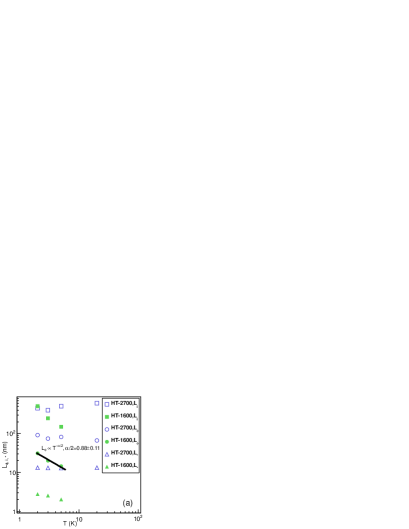
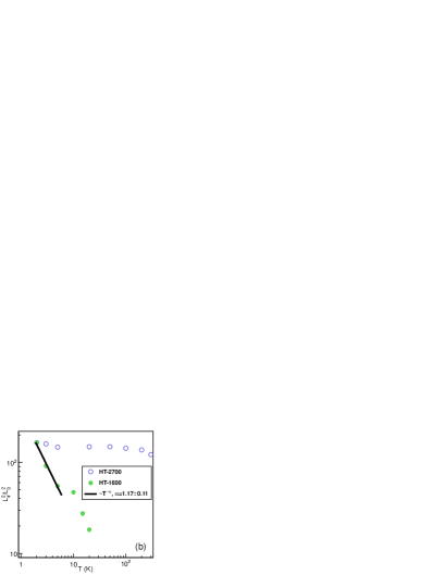
Figure 7: (a) Characteristic scattering lengths $L_{\phi,i,\ast}$ versus temperature $T$ for HT-1600 and HT-2700 nanocarbon powders. These lengths were determined using the fit parameters of the conductance versus magnetic field analysis of tables 2 and 3. For the HT-1600 sample the dephasing length is approximated by a power law $L_{\phi}\propto T^{-\alpha/2}$, where the exponent $\alpha=1.76\pm 0.22$. (b) The square of the normalized, inelastic scattering length $L_{\phi}^{2}/L_{0}^{2}$ versus temperature $T$ for the HT-1600 and HT-2700 nanocarbon powders as extracted from the scaling function equation (3). For the HT-1600 sample, the fit to a power law $L_{\phi}^{2}\propto T^{-\alpha}$, where $\alpha=1.17\pm 0.11$, is shown as a solid line. In this method, the $L_{0}$ parameter is undetermined and sample specific.

Whereas the phase coherence length $L_{\phi}$ of the HT-2700 sample shows only a weak temperature dependence, for the HT-1600 sample the temperature dependence follows $L_{\phi}\propto T^{-\alpha/2}$ with the exponent extracted from the fitted conductance parameters, $\alpha=1.76\pm 0.22$, being somewhat higher than that found from the scaling analysis, $\alpha=1.17\pm 0.11$. These fits for the exponents are shown as solid lines in figures 7 (a) and 7 (b).

5 Discussion

The investigated composite samples are disordered macroscopic objects consisting of disk- and cone- shaped nanocarbon particles which are randomly oriented in sample. The particle volume fraction in the samples (section 2.2) was high and well above the percolation threshold [42] to ensure many conducting paths through the macroscopic sample. The transport properties of these samples are reproducible.

TEM images of single grains or particles show that the crystalline quality is considerably improved on heat treatment. It should be noted that the TEM images in figure 1 only shows the layering structure near the rim of the particles where the layers bend and are perpendicular to the disk surface [30]. The nanocrystalline structure may then be much better away from the edges and near the core of the particles [19].

The resistivities of samples at temperature $T=2\>\mathrm{K}$, $\rho_{1600}=6.9\times 10^{-4}\>\Omega\mathrm{m}$ and $\rho_{2700}=5.45\times 10^{-4}\>\Omega\mathrm{m}$, are higher than the typical critical resistivity of metals $\rho\approx 1\times 10^{-6}\>\Omega\mathrm{m}$ [6] and are also higher than Mott’s criterion [6, 10] for minimum metallic conductivity, which corresponds to $\rho\left(\mathrm{metal}\right)<\approx 5\times 10^{-5}\>\Omega\mathrm{m}$. In such cases a direct application of quasiclassical theories is not possible and quantum corrections are needed [6].

As shown in figure 3, for the temperature range $10\leq T\leq 300\>\mathrm{K}$, the reduced activation energy $W(T)$ increases with $T$, which shows that both samples belong in the metallic regime [10]. For the HT-2700 sample there is a trend of $W(T)$ decreasing with $T$ below about 7 K, which may be interpreted as crossover toward an insulating type of behaviour. The wide scattering of the points for the HT-1600 sample prohibits any conclusion about possible shift in the behaviour at low temperature for this sample.

At low temperatures, $2\leq T\leq 40\>\mathrm{K}$, the changes in resistance with temperature are relatively small, as quantified by the paramater $\gamma=\rho\left(1.9\>\mathrm{K}\right)/\rho\left(40\>\mathrm{K}\right)$. We find $\gamma_{1600}=1.04$, $\gamma_{2700}=1.08$. If $\gamma<2$ the sample belongs in a metallic regime and the density of carriers is high [3]. The data could not be fitted to any exponential temperature dependence. This implies that our experimental data cannot be discussed within the frame of variable-range hopping transport [6, 10]. Similar properties were observed in a single graphite microdisk [43] and for nanocrystalline graphite [44].

In zero magnetic field, the temperature dependence of the resistance, $R(T)$, of the HT-1600 sample shown in figure 2(a) and of the HT-2700 sample in figure 2(b) are approximated by the same equation (1). In these samples inelastic scattering events due to interfering paths of electrons may give a contribution to the resistance at finite $T$, which is absent for finite magnetic fields $H>0$ [5, 10].

These resistance behaviours reveal 3D electron transport for temperature $30<T<300\>\mathrm{K}$. We initially considered that Kawabata’s theory of negative MR [12] in 3D might explain the results shown in figures 4 and 5. The theory predicts asymptotic forms $\Delta G\propto\sqrt{B}$ for large magnetic fields and $\Delta G\propto B^{2}$ for small magnetic fields [5, 8, 10, 12]. The experimental data for the two samples shown in figures 4 and 5 could not be approximated by the the asymptotic forms of the Kawabata equation neither in weak nor in strong magnetic fields (see section 4.2). We have also verified that these data cannot be modeled using the theory of Hikami at al [11].

The observed layered structure of the nanocarbon particle and the earlier finding that 3D carbon conductors can behave as 2D systems [10] but different from WL in 2D electron gas [7, 11], inspired us to look into models used for electron transport in 2D multilayer graphene [15, 45]. We have successfully applied the equation (4), which was originally derived to explain transport in single layer graphene [22], to approximate the results shown in figures 4 and 5. Magnetoconductivity in figure 5 resembles the results presented for multilayer epitaxial graphene reported by Friedman et al. [45] and by Singh et al. [15]. Since our samples at $T=2\,\mathrm{K}$ have conductivities that are several tenfold times the quantum conductivity $\sigma_{0}=2e^{2}/h$, they consist of very many conducting paths that each may be partly graphene-like [14, 15, 23, 45, 46]. For example, at similar $B-T$ conditions the samples reported by Singh et al. [15] consisting of about $20$ graphene layers show thousand times lower conductivity then our HT-2700 sample in figure 6. After conductance normalization (equation 4) the experimental data are well approximated by the McCann model [22] for a wide range of temperatures and magnetic fields. Our magnetoconductivity results in figure 6 (a) may be compared to experimental data for graphene [13], rippled graphene [47], bilayer graphene [48] or multilayered graphene [15]. It may be noted that the model for bilayer graphene [48] which has a positive sign of the third term in equation (4), clearly did not fit our experimental data.

Typical sizes of most of the nanocarbon particles were $\sim 0.3-3.0\,\mu\mathrm{m}$ with the thickness of the walls in the range $10-50$ nm. This thickness of our nanoparticles is comparable but slightly larger than the thickness of multilayered epitaxial graphene samples [15, 45]. However, although their remaining external dimensions are essentially smaller than the dimensions of the multilayer samples [15, 45], the grain size of our material may be approaching that of multilayer graphene. The calculated dephasing lengths $L_{\phi}$ (figure 7 (a)) are smaller than the in-plane carbon particle sizes but comparable or larger than typical particle thickness. For example, the typical lengths $L_{\phi}$ in HT-1600 ($14<L_{\phi}<31\>\mathrm{nm}$) and HT-2700 ($66<L_{\phi}<92\>\mathrm{nm}$) are smaller than the diameter of the disk- or cone-shaped particles. These are reasons why our nanosized objects, graphite-like nanosize crystalities [49], and the multilayer graphene samples [15, 45] can be considered to be quasi-2D objects. The intervalley $L_{i}$ and intravalley $L_{\ast}$ scattering lengths found here are comparable to those found in graphene [13, 38]. The dephasing length $L_{\phi}$ is smaller than the values reported for graphene [13, 38] and multilayer graphene [15]. We have found that $L_{\phi}<L_{i}$, which is not typical for graphene.

The temperature dependence of dephasing length $L_{\phi}$ can be determined using an alternative approach based on magnetoconductivity scaling [8, 10]. For all samples the magnetoconductivities at different temperatures (figures 4(b) and 5(b)) scale using the universal scaling form equation (3) with a single parameter $c=1/B_{\phi}$. We found that our samples follow a scaling relation [8, 10] $\Delta G/G_{0}=-Af\left(B/B_{\phi}\right)$ with $A=\left(1/B_{\phi}\right)^{0.6}$, which give rise to the excellent data collapse in figure 4(b). In contrast to the previous results [8, 10], our data do not scale onto a single universal curve. For the HT-1600 sample we found two scaling functions which divide the investigated temperature range into low ($T<T_{C}$) and high ($T>T_{C}$) temperature intervals. The critical temperature falls in the range $30<T_{C}<50\>\mathrm{K}$. For the HT-2700 sample we found that except data at low temperatures $T<20\>\mathrm{K}$ and low magnetic fields $B<3\>\mathrm{T}$ all remaining data fall onto one universal function. The deviations from universal scaling forms are a consequence of WL effects.

From the scaling form we determined $B_{\phi}$, or equivalently, the square of the phase coherence length $L_{\phi}$ since $B_{\phi}^{-1}\propto L_{\phi}^{2}$. The temperature dependence of $L_{\phi}^{2}$ reveals information about electron scattering mechanisms. The $B_{\phi}$-field vs. temperature $T$ at low temperatures obeys the scaling $B_{\phi}^{-1}\propto L_{\phi}^{2}\propto\tau_{\phi}\propto T^{-\alpha}$. In figure 7 (b) we determined the scaling exponent $\alpha=1.17\pm 0.11$ for the HT-1600 samples. For HT-1600 sample and temperature $2\leq T\leq 5\>\mathrm{K}$ (figure 7 (a)) a slightly higher value, $\alpha\approx 1.76$, was determined based on the fits to equation (4). Considering these two methods to be equivalent, we find the scaling exponent of the HT-1600 sample to be in the range $\alpha=1.2-1.8$. The scaling exponent of the HT-1600 sample is then near the prediction of the exponent $\alpha=1.5$ for e-e scattering in the dirty limit [8, 9]. However, experiments on twisted bilayer graphene [16] found that the dephasing rate was dominated by electron-electron Coulomb interaction with $\tau_{\phi}^{-1}\propto T^{2}$, i.e. $\alpha=2$. For the HT-2700 sample, the coherence lengths $L_{\phi}$ determined using the two different methods show only a weak temperature dependence, as seen in figure 7. Similar results were observed in a graphite microdisk [43] and in multilayer epitaxial graphene on SiC [15, 45]. This property was attributed to electronically decoupling of graphene layers [15, 45].

The band structure around the Dirac points in monolayer graphene is linear while in bilayer AB stacked graphene it is quadratic [1, 48]. Multilayer regularly ABA or ABC stacked graphene show a band structure which depends on the number of graphene layers, but for number of layers $n>11$ the band structure is similar to graphite [50]. However, linear band spectrum is preserved when graphene layers are misoriented [24, 25, 51, 52], i.e., adjacent rotated planes become electronically decoupled [52]. In our nanoparticles faceting angles of $\sim 22^{\circ}$ were observed [19], which fits well with the second commensurate rotation $\theta_{2}=21.7^{\circ}$ found in the calculations by Loopes dos Santos et al. [24]. Electronically decoupled graphene layers were observed in multilayer graphene [15, 45] and recently very high mobilities in multilayer 2D samples that look similar to ours were reported and interpreted to be a consequence of electronic decoupling of turbostratic graphene layers [53]. In those samples the reported mobilities of inner layers may approach that of suspended graphene. These results support the idea that nearly non-interacting parallel graphene layers may exist in several types of multilayered graphene. Thus, the model of decoupled graphene layers used to approximate magnetoconductivities in equation (4) may be justified in the present case.

Electron interactions in certain multilayer graphene samples, e.g., our HT-2700 sample in figures 7 and the epitaxial graphene of Singh et al. [15], do not behave conventional because the dephasing length $L_{\phi}$ is almost independent of temperature. In graphene flakes the electron dephasing rate obeys the usual linear $T$-dependence $\tau_{\phi}^{-1}\propto T$ [13]. Tikhonenko et al. [13] concluded that electron interference in graphene is significantly different from other 2D systems, however e-e interaction does not show unconventional behaviour. Analyzing our results and the results of other groups one may conclude that unconventional temperature behaviour of dephasing length $L_{\phi}$, or dephasing time $\tau_{\phi}$, is a typical property of turbostratic-like graphene layers. To explain this specific behaviour a new theoretical approaches will be needed. Very recent models of twisted bilayer graphene [17] have predicted novel effects such as exciton swapping between sheets.

In the case of inelastic electron scattering [5] magnetoconductivity measurements should be consistent with resistivity versus temperature measurements. The exponent $\beta$ in equation (1) depends on scattering mechanism. For $L_{\phi}^{2}\propto T^{-\alpha}$, it is expected that $\beta=\alpha/2$. Here, the $\beta$ values of our samples are found in table 1 and $\alpha$ values are shown in figures 7 (a) and 7 (b). The HT-1600 sample shows the best consistency between the these exponents, $\alpha\approx 1.76$ and $\beta\approx 0.84$. The exponents of the HT-2700 samples are not consistent with inelastic electron scattering in 3D [5].

6 Conclusions

Electronic transport in macroscopic bulk composite samples containing nanocarbon disks and cones in PMMA has been investigated using magnetotransport measurements in order to find characteristic electron scattering lengths and their temperature dependencies. We found that the magnetotransport properties are strongly dependent on the increase in the fraction of crystalline phases in the nanocarbon particles after heat treatment of the particles. We applied the McCann theory of magnetoconductivity of single layer graphene to approximate the low temperature data and interpret the changes of magnetoconductivity for the nanocarbon heat-treated at $1600^{\circ}$ C as a result of temperature variations of the electron scattering length $L_{\phi}$. We found the exponent $\alpha$ in the range 1.17-1.76 for the temperature dependence of $L_{\phi}$, $L_{\phi}^{2}\propto T^{-\alpha}$. The material heat-treated at $2700^{\circ}$ C did not show any such clear changes at low temperatures. The characteristic electron scattering lengths are typically less than about 100 nm, much smaller than the particle sizes.

References

References

- [1] Neto A H C, Guinea F, Peres N M R, Novoselov K S and Geim A K 2009 Rev. Mod. Phys. 81 109
- [2] Peres N M R 2010 Rev. Mod. Phys. 82 2673
- [3] Das Sarma S, Adam V, Hwang E H and Rossi E 2011 Rev. Mod. Phys. 83 407
- [4] Soule D 1958 Phys. Rev. 112 698
- [5] Lee P A and Ramakrishnan T V 1985 Rev. Mod. Phys. 57 287
- [6] Imry Y Introduction to Mesoscopic Physics (Oxford University Press, New York, 1997)
- [7] Altshuler B L, Khmeľnitzkii D, Larkin A I and Lee P A 1980 Phys. Rev. B 22 5142
- [8] Vora P M, Gopu P, Rosario-Canales M, Pérez C R, Gogotsi Y, Santiago-Avilés J J and Kikkawa J M 2011 Phys. Rev. B 84 155114
- [9] Menon R, Yoon C O, Moses D, Heeger A J and Cao Y 1993 Phys. Rev. B 48 17685
- [10] Vavro J, Kikkawa J M and Fischer J E 2005 Phys. Rev. B 71 155410
- [11] Hikami S, Larkin A I and Nagaoka Y 1980 Progr. Theor. Phys. 63 707
- [12] Kawabata A 1980 Solid State Commun. 34 431
- [13] Tikhonenko F V, Horsell D W, Gorbachev R V and Savchenko A K 2008 Phys. Rev. Lett. 100 056802
- [14] Baker A M R, Alexander-Webber J A, Altebaeumer T, Janssen T J B M, Tzalenchuk A, Lara-Avila S, Kubatkin S, Yakimova R, Lin C -T, Li L -J and Nicholas R J 2012 Phys. Rev. B 86 235441
- [15] Sevak Singh R, Wang X, Chen W and Wee A T S 2012 Appl. Phys. Lett. 101 183105, ibid. 2013 Appl. Phys. Lett. 103 049902
- [16] Meng L, Chu Z -D, Zhang Y, Yang J -Y, Dou R -F, Nie J -C and He L 2012 Phys. Rev. B 85 235453
- [17] Sarrazin M and Petit F 2014 Eur. Phys. J. B 87 26
- [18] Krishnan A, Dujardin E and Treacy M 1997 Nature (London) 388 451
- [19] Garberg T, Naess S N, Helgesen G, Knudsen K D, Kopstad G and Elgsaeter A 2008 Carbon 46 1535
- [20] Fung A W P, Wang H, Dresselhaus M S, Dresselhaus G, Pekala R W and Endo M 1994 Phys. Rev. B 49 17325
- [21] Kuznetsov V L, Butenko Y V, Chuvilin A L, Romanenko A I and Okotrub A V 2001 Chemical Physics Letters 336 397
- [22] McCann E, Kechedzhi K, Faľko V I, Suzuura H, Ando T and Altshuler B L 2006 Phys. Rev. Lett. 97 146805
- [23] Wu X, Li X, Song Z, Berger C and de Heer W A 2007 Phys. Rev. Lett. 98 136801
- [24] Lopes dos Santos J M B, Peres N M R and Castro Neto A H 2007 Phys. Rev. Lett. 99 256802
- [25] Latil S, Meunier V and Henrard L 2007 Phys. Rev. B 76 201402
- [26] Hughdahl J, Hox K, Lynum S, Hildrum R and Norvik M Norwegian Patent No. NO325686 (B1), issued 1999.09.23
- [27] Svåsand E, Helgesen G and Skjeltorp A T 2007 Colloids and Surfaces A: Physicochem. Eng. Aspects 308 67
- [28] Heiberg-Andersen H, Walker G W, Skjeltorp A T, Naess S N in Handbook of Nanophysics 5 - Functional Nanomaterials edited by K.D. Sattler, chap. 25, (CRC Press, Boca Raton, 2011)
- [29] Naess S N, Elgsaeter A, Helgesen G and Knudsen K D 2009 Sci. Technol. Adv. Mater. 10 065002
- [30] Hage F S, Ph.D. thesis, University of Oslo, 2013
- [31] Gogotsi Y, Dimovski S and Libera J A 2002 Carbon 40 2263
- [32] Iijima S, Yudasaka M, Yamada R, Bandow S, Suenaga K, F. Kokai F and Takahashi K 1999 Chem Phys. Lett. 309 165
- [33] Warren B E, X-Ray Diffraction (Dover, New York, 1990)
- [34] Ekşioǧlu B and Nadarajah A 2006 Carbon 44 360
- [35] Amelinckx A, Luyten W, Krekels T, Van Tendeloo G and Van Landuyt J 1992 Crystal Growth 121 543
- [36] Černák J, Helgesen G, Skjeltorp A T, Kováč J, Voltr J and Čižmár E 2013 Phys. Rev. B 87 014434
- [37] Tikhonenko F V, Kozikov A A, Savchenko A K and Gorbachev R V 2009 Phys. Rev. Lett. 103 226801
- [38] Pal A N, Kochat V and Ghosh A 2012 Phys. Rev. Lett. 109 196601; ibid. Supplemental Material at http://link.aps.org/supplemental/10.1103/PhysRevLett.109.196601
- [39] Kozikov A A, Horsell D W, McCann E and Faľko V I 2012 Phys. Rev. B 86 045436
- [40] Cai J Z, Lu L, Kong W J, Zhu H W, Zhang C, Wei B Q, Wu D H and Liu F 2006 Phys. Rev. Lett. 97 026402
- [41] Duan F and Guojun V Introduction to Condensed Matter Physics (World Scientific, Singapore 2005)
- [42] Stankovich S, Dikin D A, Dommett G H B, Kohlhaas K M, Zimney E J, Stach E A, Piner R D, Nguyen S T and Ruoff R S 2006 Nature (London) 442 282
- [43] Dujardin E, Thio T, Lezec H and Ebbesen T W 2001 Appl. Phys. Lett. 79 2474
- [44] Mandal G, Srinivas V and Rao V V 2013 Carbon 57 139
- [45] Friedman A L, Tedesco J L, Campbell P M, Culbertson J C, Aifer E, Perkins F K, Myers-Ward R L, Hite J K, Eddy C R, Jernigan G G and Gaskill D K 2010 Nano Lett. 10 3962
- [46] Lara-Avila S, Tzalenchuk A, Kubatkin S, Yakimova R, Janssen T J B M, Cedergren K, Bergsten T and Faľko V 2011 Phys. Rev. Lett. 107, 166602
- [47] Lundeberg M B and Folk J A 2010 Phys. Rev. Lett. 105 146804
- [48] Gorbachev R V, Tikhonenko F V, Mayorov A S, Horsell D W and Savchenko A K 2007 Phys. Rev. Lett. 98 176805
- [49] Romanenko A I, Anikeeva O B, Kuznetsov V L, Obrastsov A N, Volkov A P and Garshev A V 2006 Solid State Commun. 137 625
- [50] Partoens B and Peeters F 2006 Phys. Rev. B 74 075404
- [51] Ohta T, Bostwick A, McChesney J L, Seyller T, Horn K and Rotenberg E 2007 Phys. Rev. Lett. 98 206802
- [52] Hass J, Varchon F, Millán-Otoya J, Sprinkle M, Sharma N, de Heer W A, Berger C, First P N, Magaud L, and Conrad E 2008 Phys. Rev. Lett. 100 125504
- [53] Hernandez Y R, Schweitzer S, Kim J, Patra A J, Englert J, Lieberwirth I, Liscio A, Palermo V, Feng X, Hirsch A, Kläui M M and Müllen L http://arxiv.org/ftp/arxiv/papers/1301/1301.6087.pdf