A MATHEMATICA PACKAGE FOR CALCULATION OF ONE-LOOP PENGUINS IN FCNC PROCESSES

Abstract

In this work, we present a Mathematica package Peng4BSM@LO which calculates the contributions to the Wilson Coefficients of certain effective operators originating from the one-loop penguin Feynman diagrams. Both vector and scalar external legs are considered. The key feature of our package is the ability to find the corresponding expressions in almost any New Physics model which extends the SM and has no flavour changing neutral current (FCNC) transitions at the tree level.

PACS Nos.: 11.25.Hf, 123.1K

1 Introduction

The flavour changing neutral current (FCNC) processes attract a lot of interest from both the theoretical and experimental side. Such transitions are absent in the SM at the tree level and, thus, are suppressed in comparison with the charged current processes. Due to this, FCNC can be used as an excellent probe of New Physics, which can considerably alter the predictions of the SM. At the moment, no significant deviations are found. Consequently, these rare processes impose very important constraints on Beyond-the-SM (BSM) physics. Typical examples are the $b\to s\gamma$ [1, 2, 3] and $B_{s}\to\mu\mu$ decays [4, 5, 6] which are used in different studies of various supersymmetric extensions of the SM. Since new particles predicted by BSM models are usually much heavier than the SM ones, the corresponding (short-distance) contribution to FCNC amplitudes can be absorbed into the Wilson coefficients of the operators which enter into the weak effective Hamiltonian [7].

In order to calculate the Wilson coefficients for a particular FCNC process in supersymmetric or any two-higgs doublet models, one can use different codes available on the market, e.g., SuperIso [8, 9, 10], SUSY_FLAVOUR [11, 12] or SPheno_v3 [13] (see also, Ref. [14]).

We created a Mathematica package Peng4BSM@LO which can be used together with FeynArts [15, 16, 17, 18, 19] and FeynCalc [20] to address the same problem. However, contrary to the above-mentioned flavour codes, our routines give an opportunity to obtain the expression for the Wilson coefficients in almost any renormalizable BSM model, which can be implemented in FeynArts format with the help of FeynRules [21, 22, 23], LanHEP [24, 25] or SARAH [26, 27, 28, 29]. However, it should be stressed from the very beginning that a BSM model should not have the tree-level FCNC coupling, which corresponds to the considered FCNC (sub)process. Only one-loop generated transitions are taken into account.

In Sec.2, we define our notation and present generic operators contributing to the effective Hamiltonian. In Sec.3, we introduce the programming instruments, our method to define and calculate the Wilson coefficients and describe and explain the structural diagram of the package Peng4BSM@LO. In Sec.4, the basic usage of the functions of Peng4BSM@LO is presented. In Sec.5, we carry out some benchmark tests of the package by reproducing known expressions for penguins with external $Z$-boson, photon $\gamma$ [30] and the Higgs field $H$ [31] in the SM. In addition, the gluino contribution in MSSM with non-minimal flavour violation is recalculated for $b\to s\gamma$ process [32]. In A, we give characteristics of the package and the reference, from which one may download it. In B, commands’ descriptions of the main procedures are stated. Then subsequently, in C, descriptions of the auxiliary procedures and definitions of program parameters are clarified.

2 Generic operators

In Peng4BSM@LO, we consider the following generic effective local operators and their form factors, $\left(N^{0,c}_{a,b}\right)_{L,R}$, $\left(E^{0,c}_{a,b}\right)_{L,R}$, $\left(E^{2,c}_{a,b}\right)_{L,R}$, $\left(M^{1,c}_{a,b}\right)_{L,R}$. The scalar operators are of the form

$$H_{eff}\ni\left(\bar{F}_{a}^{\prime}P_{L,R}F_{b}S_{c}\right)\left(N^{0,c}_{a,b}\right)_{L,R}$$ (1)

where $S$ is a neutral scalar boson field and $P_{L,R}=(1/2)(1\mp\gamma^{5})$ are the projection operators. The monopole operators which conserve chirality are of the form

$$H_{eff}\ni\left(\bar{F}_{a}^{\prime}\gamma^{\mu}P_{L,R}F_{b}\right)\left[\left(E^{0,c}_{a,b}\right)_{L,R}g^{\mu\nu}+\left(g^{\mu\nu}q^{2}-q^{\mu}q^{\nu}\right)\left(E^{2,c}_{a,b}\right)_{L,R}\right]V^{c}_{\nu}$$ (2)

and the dipole operators which flip chirality are

$$H_{eff}\ni\left(\bar{F}_{a}^{\prime}\sigma^{\mu\nu}P_{L,R}F_{b}q_{\mu}V^{c}_{\nu}\right)\left(M^{1,c}_{a,b}\right)_{L,R}.$$ (3)

Here the metric tensor is defined as $g^{\mu\nu}=\mathrm{diag}(1,-1,-1,-1)$, $\sigma^{\mu\nu}\equiv(i/2)\left[\gamma^{\mu},\gamma^{\nu}\right]$, and $q_{\mu}$ is the outgoing momentum of a neutral vector boson $V$ entering into the operators. Fermions of different families are denoted by $F$ and $F^{\prime}$, $a,~{}b,~{}c$ are some, e.g., color indices. From the form factors one can easily extract the corresponding Wilson coefficients. This kind of operators originates from the expansion of penguin amplitudes in external momenta, so that ($N^{0}$, $E^{0}$), $M^{1}$ and $E^{2}$ correspond to the zeroth, first and second order terms in this expansion, respectively.

3 Structure of Peng4BSM@LO

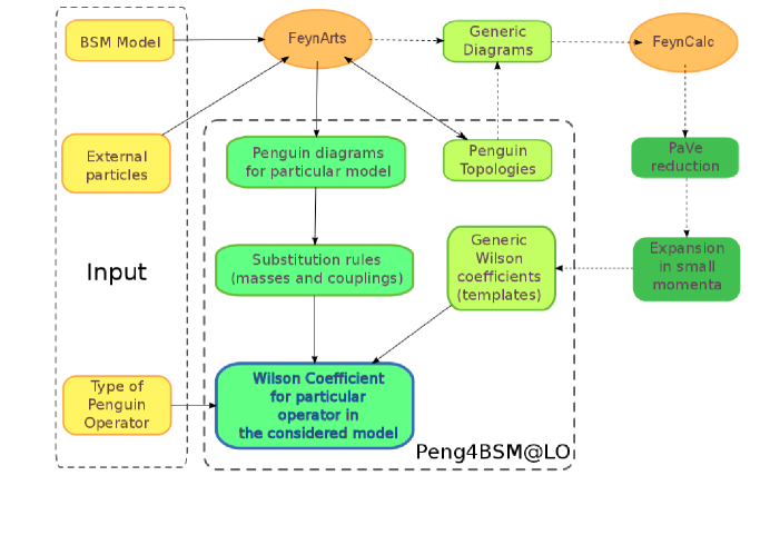
Figure 1: The new package to calculate and define Wilson coefficients for the one-loop penguin diagrams in FCNC processes.

Our paradigm (see Fig. 1) is inspired by FeynArts hierarchy of fields (Generic, Classes, and Particles) and is based on the fact that the Lorentz structure of Feynman vertices is fixed only by the type of participating particles, so one can define and calculate generic Wilson coefficients originating from generic diagrams. The corresponding amplitudes involve generic couplings which can be substituted later by actual expressions. One should keep in mind that we heavily rely on the Lorentz structures defined in the generic model file Lorentz.gen distributed with FeynArts. The restriction applies primarily to the LanHEP package which generates its own generic model file. Due to this, additional effort is required to rewrite Feynman rules produced by LanHEP to make them consistent with our code.

With the help of FeynArts we generate so-called generic diagrams (see Fig. 2). Then we reformulate the generic amplitudes by means of FeynCalc in terms of the fundamental integrals of Passarino-Veltman’s [33] which we expand in the limit of vanishing external momenta in order to obtain the generic Wilson coefficients. These generic Wilson coefficients serve as templates and can be used in any model. Given the corresponding expressions, the substitution rules for particular diagrams and amplitudes can be applied and the Wilson coefficients for a particular model can be obtained.

Let us mention that we restrict the package to the Feynman gauge, in which gauge propagators have very simple structure and, as a consequence, the complexity of the templates is significantly reduced. In addition, no unphysical gauge-parameter dependent masses appear in individual diagrams.

Figure 2: The one-loop generic diagrams, where $F$ is a a fermion, $S$ is a scalar and $V$ is a vector. We do not consider the self-energy insertions in the neutral vector boson leg, since we assume that there is no tree-level FCNC. The corresponding diagrams for $F\to F~{}S$ transition are obtained by replacing the external vector boson $V$ with a scalar field $S$.

As we see from Fig. 1, in order to obtain a contribution to $N^{0}$, $E^{0,2}$ or $M^{1}$, one should define the model and the corresponding operator with external particles $F_{a},F_{b}$, $V_{c}$ or $S_{c}$ from Eqs. (1),(2), and (3). Given this input, the package can be used in the following way. First of all, one should construct the relevant Feynman diagrams by calling PengInsertFields [$\{F_{b}\}$ $\to\{F_{a},B_{c}\},{\tt Model}\to\mbox{{\tt MOD}}]$ where the boson $B_{c}$, is either a vector one, $V_{c}$, or a scalar one denoted by $S_{c}$. The procedure is similar to InsertFields of FeynArts but uses a predefined set of topologies PenguinTopologies (see Fig. 3). The model is specified by the option Model $\to$ MOD. The corresponding Feynman rules in FeynArts notation are taken from the file MOD.mod. The function PengInsertFields accepts the same options as InsertFields, so one can restrict the set of generated diagrams, e.g., by ExcludeParticles option[19] . Then, the penguin amplitudes are produced by PengCreateFeynAmp from the diagrams created with PengInsertFields. After that, one should apply ExtractPenguinSubsRules to produce a list of substitution rules for each diagram (amplitude) generated by PengCreateFeynAmp. The rules specify the actual couplings for each generic diagram (amplitude). They can be used later together with SubstituteMassesAndFeynmanRules to obtain final analytic expressions in the considered model. In order to demonstrate the features of the package, we apply it to the study of the effective $d\bar{s}Z$, $d\bar{s}\gamma$ [30] and $b\bar{b}H$ [31] vertices in the SM, and to the effective $b\bar{s}\gamma$  [32] vertex in the MSSM.

Figure 3: Penguin topologies as defined in Peng4BSM@LO.

4 Peng4BSM@LO in Use

The package Peng4BSM@LO employs FeynArts to generate the relevant diagrams. It is worth mentioning that one is not forced to use FeynCalc which was utilized by us at the intermediate stages for calculation of the generic amplitudes. However, it may be convenient to load FeynCalc to produce some nicely formatted output. In order to do so, one executes the following commands in the Mathematica FrontEnd

$$\tt In[1]:= \tt\$UseFeynCalc=True;$$ (4)

To use the package Peng4BSM@LO in the notebook, we should load it by the following command line

$$\tt In[2]:=\hskip 19.91684pt\tt{Get}["/\tt{PATH}/\tt{Peng4BSMatLO.m}"];$$ (5)

where PATH is the path to the directory with Peng4BSM@LO. After this preparation, we can specify the operator external particles in terms of FeynArts fields defined in the considered model

$$\tt In[3]:= \tt{InF=F[4,\{1,c1\}];}~{}~{}~{}(\textrm{for d-quark})$$ (6)

$$\tt{OutF=F[4,\{2,c2\}];}~{}~{}~{}(\textrm{for s-quark})$$

$$\tt{OutV=V[2]};~{}~{}~{}(\textrm{for Z-boson})$$

The next step is to distribute the fields defined in the chosen model over internal lines in the considered topologies. This is done automatically by FeynArts with the help of PengInsertFields function,

$$\tt In[4]:= \tt{diagrams=PengInsertFields[}\{\tt{InF}\}$$

$$\to\{\tt{OutF},\tt{OutV}\},\tt{Model}\to\tt{"SMQCD"]}$$

$$\tt In[5]:= \tt{Paint[diagrams,PaintLevel}\to\tt{\{Classes\},Numbering}$$ (7)

$$\to\tt{Simple,ColumnsXRows}\to\{5,2\}];$$

Here diagrams is a variable used to store the output of InsertFields and SMQCD corresponds to the full SM. For convenience, one can also draw the generated diagrams with Paint. The result of the evaluation in Eq. (4) is presented in Fig. 4. The option PaintLevel is used to choose at which level (Classes, in our example, with all up-type quarks, $u$, $c$, $t$ combined in $u_{l}$) the diagrams should be drawn. Similarly, the options Numbering and ColumnsXRows are used to format the picture .

Figure 4: The one-loop diagrams contributing to $d\bar{s}Z$ in the SM. The fields $u_{l}$, $W$, and $G$ in internal lines correspond to up-type quarks of the $l$-th generation, $W$-boson and charged would-be Goldstone boson, respectively.

Then, we use the function PengCreateFeynAmp to create amplitudes from diagrams, as we see the role of it in Sec.3.

$$\tt In[6]:=\hskip 19.91684pt\tt{penguin=PengCreateFeynAmp[diagrams]}$$ (8)

Given the output of this command the function ExtractPenguinSubsRules produces a list of substitution rules for each diagram (unevaluated amplitude) generated by PengCreateFeynAmp.

$$\tt In[7]:=\hskip 19.91684pt\tt{substrules=ExtractPenguinSubsRules[penguin]}$$ (9)

The rules substrules specify the actual couplings for each Generic diagram (amplitude). They can be used to obtain final analytic expressions in the considered model. Given substrules, one can obtain diagram-by-diagram contributions to the coefficient function of a particular operator by utilizing the SubstituteMassesAndFeynmanRules function

$$\tt In[8]:=\hskip 19.91684pt\tt{SubstituteMassesAndFeynmanRules[OP][substrules]}.$$ (10)

Here the string OP can be chosen from the set {"OpR", "OpL", "MonOpL0", "MonOpR0", "MonOpL2", "MonOpR2", "DipOpL1", "DipOpR1"}. The scalar operators from Eq. (1) correspond to "Op{L,R}", while monopole operators from Eq. (2) correspond to "MonOp{L,R}{0,2}" and finally, dipole operators from Eq. (3) — to "DipOp{L,R}1" . The output of In[8] is a list of contributions to the considered Wilson coefficient for all diagrams given in Fig.2. For convenience, for every mass parameter M we introduce a dimensionless mass ratio XXX[M/CommonMass] with CommonMass equals to the W-boson mass by default. The result is obtained in dimensional regularization. In spite of the fact that individual amplitudes can have poles in the regularization parameter $\epsilon=(4-D)/2$, the sum is finite due to the absence of the tree-level FCNC.

5 Test of Peng4BSM@LO

We compared the file the results of application Peng4BSM@LO to the induced $d\bar{s}Z$ vertex in the SM (see Fig. 4) with those given in paper [30] and got perfect agreement. For this particular case, the monopole operator is $\bar{s}_{L}\gamma^{\mu}d_{L}Z_{\mu}$ as in Eq.2.6 of [30]. We also consider the $\gamma$ exchange diagrams for the induced $d\bar{s}\gamma$ vertex in the SM (see Fig. 5) for which the corresponding generic diagrams. The corresponding operators for the induced $d\bar{s}\gamma$ vertex are the monopole operators, $A_{\mu}\bar{s}\left(q^{2}\gamma_{\mu}-q_{\mu}\not q\right)P_{L}d$ and the dipole operators, $A_{\mu}\bar{s}\sigma_{\mu\nu}iq^{\nu}\left(m_{s}P_{L}+m_{d}P_{R}\right)d$ as in Eq.B.1 of [30]. The consistency checks of Peng4BSM@LO are as follows. There are no UV-divergencies in the considered form-factors. In the case of $Z$ boson only the left-handed FCNC operator is generated, i.e., $E^{0,Z}_{R}=0$. In the case of $\gamma$ quanta both $E^{0,\gamma}_{L,R}=0$. As an example, we present the expression for $E^{0}_{L}$ corresponding to the monopole operator with external $Z$-boson:

$$\left(E^{0,Z}_{c1,c2}\right)_{L}=\sum_{k=2,3}\frac{e^{3}V_{k1}V^{*}_{k2}\delta_{c1,c2}}{64\pi^{2}\cos\theta_{W}\sin^{3}\theta_{W}\left(x_{1}^{2}-1\right)^{2}\left(x_{k}^{2}-1\right)^{2}}$$

$$\times\Bigg{\{}\Big{(}x_{1}^{2}-1\Big{)}\Big{(}x_{k}^{2}-1\Big{)}\Big{[}x_{k}^{2}\Big{(}x_{k}^{2}-6\Big{)}+x_{1}^{4}\Big{(}x_{k}^{2}-1\Big{)}-x_{1}^{2}\Big{(}x_{k}^{4}-6\Big{)}\Big{]}$$

$$+x_{1}^{2}\Big{(}6x_{1}^{2}+4\Big{)}\Big{(}x_{k}^{2}-1\Big{)}^{2}\log x_{1}-\Big{(}x_{1}^{2}-1\Big{)}^{2}x_{k}^{2}\Big{(}6x_{k}^{2}+4\Big{)}\log x_{k}\Bigg{\}}.$$ (11)

The expression is obtained by summing contributions from individual diagrams calculated by means of SubstituteMassesAndFeynmanRules with OP="MonOpL0". In Eq. (5) mass ratios $x_{i}=m_{i}/M_{W}$ are introduced with $i=1,2,3$ being up-type quark family indices. The Cabibbo-Kobayashi-Maskawa (CKM) matrix $V_{ij}$ is denoted in FeynArts by $CKM(i,j)$. The Kronecker-delta in colour space is given by $\delta_{c1,c2}\equiv\textrm{IndexDelta}(c1,c2)$ with $c1$ and $c2$ being colour indices. The W-boson mass, the electric charge and sine of the Weinberg angle are denoted by $M_{W}$, $e$ and $\sin\theta_{W}$, respectively. It is worth pointing that it is crucial to use the unitarity of the CKM matrix to cancel divergent contributions to the form-factors (5). It is due to this, only $V_{21}V^{*}_{22}\equiv V_{cd}V^{*}_{cs}$ and $V_{31}V^{*}_{32}\equiv V_{td}V^{*}_{ts}$ appear in Eq. (5).

Figure 5: The one-loop diagrams contributing to $d\bar{s}\gamma$ in the SM. The fields $u_{l}$, $W$, and $G$ in internal lines correspond to up-type quarks of the $l$-th generation, $W$-boson and charged would-be Goldstone boson, respectively.

The form factor for the second order monopole operator for a massless outgoing boson, in our case it is a photon $\gamma$, is:

$$\left(E^{2,\gamma}_{c1,c2}\right)_{L}=\sum_{k=2,3}\frac{e^{3}V_{k1}V^{*}_{k2}\delta_{c1,c2}}{1152\pi^{2}M_{W}^{2}\sin^{2}\theta_{W}\left(x_{1}^{2}-1\right)^{4}\left(x_{k}^{2}-1\right)^{4}}$$ (12)

$$\times \Bigg{\{}\Big{(}1-x_{1}^{2}\Big{)}\Big{(}x_{k}^{2}-1\Big{)}\Big{[}25x_{k}^{4}-19x_{k}^{6}+x_{1}^{6}\Big{(}19-57x_{k}^{2}+32x_{k}^{4}\Big{)}$$

$$+ x_{1}^{4}\Big{(}75x_{k}^{2}-32x_{k}^{6}-25\Big{)}+x_{1}^{2}\Big{(}57x_{k}^{6}-75x_{k}^{4}\Big{)}\Big{]}$$

$$+ 4\Big{(}8-32x_{1}^{2}+54x_{1}^{4}-30x_{1}^{6}+3x_{1}^{8}\Big{)}\Big{(}x_{k}^{2}-1\Big{)}^{4}\log x_{1}$$

$$+ 4\Big{(}1-x_{1}^{2}\Big{)}\Big{(}x_{1}^{2}-1\Big{)}^{3}\Big{(}8-32x_{k}^{2}+54x_{k}^{4}-30x_{k}^{6}+3x_{k}^{8}\Big{)}\log x_{k}\Bigg{\}}.$$

Finally, a non-trivial contribution to the dipole operator for a massless photon is given by

$$\left(M^{1,\gamma}_{c1,c2}\right)_{L,R}=-\sum_{k=2,3}\frac{ie^{3}m_{s,d}V_{k1}V^{*}_{k2}\delta_{c1,c2}}{384\pi^{2}M_{W}^{2}\sin^{2}\theta_{W}(x_{1}^{2}-1)^{4}(x_{k}^{2}-1)^{4}}$$ (13)

$$\times \Bigg{\{}\Big{(}x_{1}^{2}-1\Big{)}\Big{(}x_{k}^{2}-1\Big{)}\Bigg{[}x_{1}^{6}\Big{(}-29x_{k}^{4}+31x_{k}^{2}-8\Big{)}+x_{1}^{4}\Big{(}29x_{k}^{6}-6x_{k}^{2}-5\Big{)}$$

$$+ x_{1}^{2}\Big{(}-31x_{k}^{6}+6x_{k}^{4}+7\Big{)}+x_{k}^{2}\Big{(}8x_{k}^{4}+5x_{k}^{2}-7\Big{)}\Bigg{]}$$

$$+ 12\Big{(}x_{1}^{2}-1\Big{)}^{4}x_{k}^{4}\Big{(}3x_{k}^{2}-2\Big{)}\log x_{k}-12\Big{(}3x_{1}^{2}-2\Big{)}x_{1}^{4}\Big{(}x_{k}^{2}-1\Big{)}^{4}\log x_{1}\Bigg{\}}$$

Also, we remind that in the presented equations the parameters defined in the SMQCD.mod model file are used. It is obvious that the results can be rewritten in terms of Fermi constant $G_{F}=e^{2}/(8M^{2}_{W}\sin^{2}\theta_{W})$ in order to factorize the result from the Wilson Coefficient together with the CKM matrix elements.

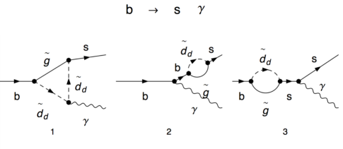
Figure 6: The one-loop diagrams contributing to $b\bar{s}\gamma$ in the FVMSSM. Down-type scalar quarks and gluino are denoted by $\tilde{d}_{d}$ ($d=1,\dots,6$) and $\tilde{g}$, respectively.

We also checked the correctness of ${\tt Peng4BSM@LO}$ in an application to the minimal supersymmetric standard model with non-minimal flavour violation (FVMSSM) [34]. The induced $b\bar{s}\gamma$ effective vertex in FVMSSM is given in Ref. [32]. The contribution due to gluino (see Fig. 6) to the operator $im_{b}\epsilon_{\mu}\bar{s}\sigma^{\mu\nu}q_{\nu}P_{R}b$ has the following form [32]:

$$\mathcal{A}_{\tilde{g}}=-\frac{\alpha_{s}\sqrt{\alpha}}{\sqrt{\pi}}C(R)e_{D}\sum_{k=1}^{6}\frac{1}{m^{2}_{\tilde{d}_{k}}}\Bigg{\{}\Gamma_{DL}^{kb}\Gamma_{DL}^{\ast ks}F_{2}[x_{k}]-\Gamma_{DR}^{kb}\Gamma_{DL}^{\ast ks}\frac{m_{\tilde{g}}}{m_{b}}F_{4}[x_{k}]\Bigg{\}},$$ (14)

where $\alpha_{s}=g_{s}^{2}/4\pi$ is the strong coupling constant, $\alpha=e^{2}/4\pi$ corresponds to the fine structure constant, $x_{k}=m_{\tilde{g}}^{2}/m_{\tilde{d}_{k}}^{2}$ with $m_{\tilde{g}}$ being the mass of gluino and $m_{\tilde{d}_{k}}$ being the mass of the scalar quarks. The charge of down-type (s)quarks is $e_{D}=-1/3$, $\Gamma_{QL,R}$ are the $6\times 3$ squark mixing matrices, $C(R)=4/3$ is the quadratic Casimir operator on the fundamental representation of $SU(3):\sum_{a}(T^{a}T^{a})_{ij}=C(R)\delta_{ij}$ with $Tr(T^{a}T^{b})=\frac{1}{2}\delta^{ab}$ and

$$F_{2}[x] = \frac{1}{12(x-1)^{4}}\left(2x^{3}+3x^{2}-6x+1-6x^{2}\log x\right)$$

$$F_{4}[x] = \frac{1}{2(x-1)^{3}}\left(x^{2}-1-2x\log x\right)$$ (15)

The equation (14) should be compared with the expression produced by our package for the operator $A_{\mu}\bar{s}\sigma^{\mu\nu}q_{\nu}P_{R}b$:

$$(M_{c1,c2}^{1,\gamma})_{R} = \frac{ieg_{s}^{2}}{288m_{\tilde{g}}^{2}\pi^{2}}\sum_{s=1}^{6}\sum_{i=1}^{3}\sum_{a=1}^{8}T^{a}_{c2,i}T^{a}_{i,c1}$$ (16)

$$\times \frac{x_{s}}{(x_{s}-1)^{4}}\Bigg{\{}m_{b}\Bigg{[}1-6x_{s}+\Big{(}3-6\log x_{s}\Big{)}x_{s}^{2}+2x_{s}^{3}\Bigg{]}R_{\tilde{d}}^{\ast s_{1},2}R_{\tilde{d}}^{s_{1},3}$$

$$- 6m_{\tilde{g}}\Big{(}x_{s}-1\Big{)}\Big{(}-1-2x_{s}\log x_{s}+x_{s}^{2}\Big{)}R_{\tilde{d}}^{\ast s_{1},2}R_{\tilde{d}}^{s_{1},6}\Bigg{\}}.$$

Here $R^{s_{1},s_{2}}_{\tilde{d}}$ is the $6\times 6$ down-type squark mixing matrix such that $R_{\tilde{d}}=\left(\Gamma_{DL}|\Gamma_{DR}\right)$. The generators of SU(3) are denoted by $T^{a}_{ij}$. In Eq. (16) we neglect explicit dependence on $m_{s}$. It is interesting to note that in the same approximation the coefficient $(M_{c1,c2}^{1,\gamma})_{L}$ of the operator $A_{\mu}\bar{s}\sigma^{\mu\nu}q_{\nu}P_{L}b$ can be obtained from Eq. (16) by the substitutions $R^{s_{1},2}_{\tilde{d}}\leftrightarrow R^{s_{1},5}_{\tilde{d}}$ and $R^{s_{1},3}_{\tilde{d}}\leftrightarrow R^{s_{1},6}_{\tilde{d}}$, which correspond to $\Gamma_{DL}\leftrightarrow\Gamma_{DR}$ replacement in Eq. (14). After some obvious colour algebra one can see that $im_{b}\mathcal{A}_{\tilde{g}}\delta_{c1,c2}=(M_{c1,c2}^{1,\gamma})_{R}$.

In Eq. (16) obtained by Peng4BSM@LO, the parameters are as in the model file, FVMSSM.mod, located in the Models subdirectory of FeynArts, i.e. the corresponding definitions of the parameters in FVMSSM.mod as the following: $m_{b}=\textrm{MB}$, $g_{s}=\textrm{GS}$, $e=\textrm{EL}$, $m_{\tilde{g}}=\textrm{MGl}$ and $R^{s_{1},s_{2}}_{u,d}=\textrm{UASf[t][$s_{1}$,$s_{2}$]}$, $T^{a}_{ij}=\textrm{SUNT[a,i,j]}$ and the sums $\sum_{i=1}^{r}$ are represented by the factors SumOver[i,r].

The third example of the application of Peng4BSM@LO is to the SM Higgs penguin with quark flavour changing interactions. For the effective Lagrangian [31]

$$\mathcal{L}^{SM}_{H\bar{s}b}=-\frac{g_{2}}{2M_{W}}H\bar{s}\bigg{[}m_{s}\left(\mathbb{g}^{L}_{H\bar{d}d^{\prime}}\right)_{sb}P_{L}+m_{b}\left(\mathbb{g}^{R}_{H\bar{d}d^{\prime}}\right)_{sb}P_{R}\bigg{]}b~{},$$ (17)

the induced $b\bar{s}H$ effective vertex in the SM (see Fig. 7) is given in [31]. The contribution corresponding to the operators $m_{s,b}H\bar{s}P_{L,R}b$ can be inferred from the matrix elements $\left(\mathbb{g}^{L,R}_{H\bar{d}d^{\prime}}\right)_{sb}$ of the factors [31]:

$$\mathbb{g}^{L}_{H\bar{d}d^{\prime}}=-\frac{g_{2}^{2}}{(16\pi^{2})}\mathbb{V}^{\dagger}f(\hat{x},y)\mathbb{V}~{}~{}~{},~{}~{}\mathbb{g}_{H_{i}\bar{d}d^{\prime}}^{R}=\left(\mathbb{g}_{H_{i}\bar{d}d^{\prime}}^{L}\right)^{\dagger}$$ (18)

where $\hat{x}=\mathbb{\hat{M}}_{u}^{2}/M_{W}^{2}$, $y=M_{H}^{2}/M_{W}^{2}$ and

$$f(\hat{x},y)=\frac{3}{4}\hat{x}+y\bigg{(}-\frac{\hat{x}^{3}\ln\hat{x}}{4(1-\hat{x})^{3}}+\frac{\hat{x}^{2}\ln\hat{x}}{2(1-\hat{x})^{3}}-\frac{\hat{x}^{2}}{8(1-\hat{x})^{2}}+\frac{3\hat{x}}{8(1-\hat{x})^{2}}\bigg{)}$$ (19)

Hereby the up- and down-type $3\times 3$ diagonal quark mass matrices are denoted by $\mathbb{\hat{M}}_{u}$ and $\mathbb{\hat{M}}_{d}$, respectively, $M_{H}$ is the Higgs boson mass and $\mathbb{V}$ corresponds to the CKM matrix.

Figure 7: The one-loop diagrams contributing to $b\bar{s}H$ in the SM.

Taking into account Eq. (18), the expression in Eq. (17) can be compared with the result produced by the package Peng4BSM@LO for the effective $b\bar{s}H$ vertex. In the limit $m_{u}=m_{c}=0$ one has

$$(N^{0,H}_{c_{1},c_{2}})_{L,R}=\frac{e^{3}m_{s,b}V_{33}V^{*}_{32}\delta_{c1,c2}}{256M_{W}\pi^{2}\sin^{3}\theta_{W}}$$

$$\times\bigg{\{}6x_{3}+\frac{y}{(-1+x_{3})^{3}}\bigg{[}-3x_{3}+4x_{3}^{2}-4x_{3}^{2}\ln x_{3}-x_{3}^{3}+2x_{3}^{3}\ln x_{3}\bigg{]}\bigg{\}}$$ (20)

where $x_{3}=m_{t}^{2}/M_{W}^{2}$, $y=M_{H}^{2}/M_{W}^{2}$ and $e=g_{2}\sin\theta_{W}$. The equivalence between the results of Ref. [31] and the output of the package is obvious in the considered limit: $-\frac{g_{2}}{2M_{W}}m_{s,b}(\delta_{c_{1},c_{2}}.g^{L,R}_{H\bar{s}b})=(N^{0,H}_{c_{1},c_{2}})_{L,R}$. The comparison of Eqs. (18) and (5) is affirmative for Peng4BSM@LO.

In addition, we would like to mention that our package correctly reproduces the general results for $f_{1}f_{2}\gamma$ vertex [35] in QED with additional scalar boson.

6 Conclusion

We present the new package which we called Peng4BSM@LO. Peng4BSM@LO is written in Mathematica and works with FeynArts and/or FeynCalc. The package defines and calculates contributions to the Wilson coefficients of particular operators for the one-loop penguin diagrams in FCNC processes.

We conducted thorough testing of the package and reproduced known results for the induced $d\bar{s}Z$ and $d\bar{s}\gamma$ vertices in the SM [30], for the gluino contribution to $b\bar{s}\gamma$ in the MSSM with non-minimal flavour violation [32], and for the induced $b\bar{s}H$ vertex in the SM [31]. This serves as a validity check of our code.

The advantage of the package is that it relies on the general Lorentz structure of the penguin amplitudes and, as a consequence, can be used to evaluate the Wilson coefficients in any renormalizable model which extends the SM.

The next steps are the calculation of the box diagrams and implementation of the Flavour Les Houches Accord [14] output, which allows one to carry out a full calculation of flavour observables.

Appendix A Program Summary

• Title of program: The name of Peng4BSM@LO is the abbreviation of penguin diagrams for Beyond the Standard Model (SM) in the leading order.

• Available from: http://theor.jinr.ru/~hanif/peng4bsm@lo/

• Programming Language: Mathematica

• Computer: Any computer where Mathematica 8 and newer is running.

• Operating system: Windows, Linux, MacOSX.

• Number of bytes in distributed program including test data etc.: Peng4BSMatLO.m is $\sim$1 065 457 bytes, test_Peng4BSMatLO.nb is $\sim$673 655 bytes.

• Distribution format: ASCII

• External routines/libraries: FeynArts 3.7 or FeynCalc 8.2

• Keywords: Penguin, BSM, Beyond the Standard Model, the SM, the Standard Model, FCNC, Wilson Coefficients, Effective Hamiltonian, OPE, Operator Product Expansion, CP violation.

• Nature of physical problem: FCNC processes are absent in the SM at the tree level and, thus, are suppressed in comparison to the charged current processes. Due to this, FCNC can be used as an excellent probe of New Physics which can considerably alter the predictions of the SM. The rare processes impose very important constraints on Beyond-the-SM (BSM) physics.

• Method of solution: Peng4BSM@LO uses Mathematica to evaluate relevant contributions to the considered Wilson coefficients from penguin diagrams in the SM and Models Beyond the SM.

• Restrictions: The calculations are restricted to the case of renormalizable Quantum Field Theories quantized in Feynman gauge. The standard generic model file, Lorentz.gen, distributed with FeynArts should be used.

• Typical running time: For all operations the running time does not exceed $\sim$60 seconds for the SM and the MSSM which we have chosen for testing. However, the running time significantly depends on the number of parameters and fields of the chosen model.

Appendix B Description of the Main Procedures

• PengInsertFields[{InF} $\to$ {OutF, OutV}, Model -> MOD]

  General: Equivalent to the FeynArts function InsertFields and is used to construct all Feynman penguin-type diagrams in a particular model for a particular set of external fields from a predefined set of topologies PenguinTopologies.

  Input: InF=$F_{a}$, OutF=$F^{\prime}_{b}$, and OutV=$V_{c}$ specify external fermions and vector fields (see Eqs. (2)-(3)), which are used to construct the corresponding induced operator, MOD is a FeynArts model. Accepts the same options as InsertFields.

  Output: TopologyList[…] — a hierarchical list of penguin-type Feynman diagrams in FeynArts notation.

• PengCreateFeynAmp[ diagrams ]

  General: Similar to the FeynArts function CreateFeynAmp, which produces analytic expressions for amplitudes given the diagrams diagrams created with the help of InsertFields.

  Input: diagrams — diagrams created by PengInsertFields. Accepts the same options as CreateFeynAmp

  Output: PengFeynAmpList[…][…] — a list of analytic expressions for Generic amplitudes together with the required substitution rules.

• ExtractPenguinSubsRules[ penguins ]

  General: Extracts a list of substitution rules for each amplitude from the output of PengCreateFeynAmp. The rules specify the actual couplings for each Generic diagram (amplitude). In addition, information about the required Generic diagram is stored.

  Input: penguins — the output of PengCreateFeynAmp.

  Output: PenguinSubsRules[…][…] — a list of substitution rules for each diagram (amplitude) generated by PengCreateFeynAmp.

• SubstituteMassesAndFeynmanRules[OP][ substrules ]

  General: Applies the substitution rules to the predefined Generic coefficient function specified by tag OP, given the rules generated by ExtractPenguinSubsRules.

  Input: OP = { "OpL" | "OpR" | "MonOpL0" | "MonOpR0" | "MonOpL2" | "MonOpR2" | "DipOpL1" | "DipOpR1" } — the operator type, substrules — the output of ExtractPenguinSubsRules.

  Output: A list with diagram-by-diagram contributions to the coefficient functions of the specified operator OP.

Appendix C Description of the Auxiliary Procedures and Definitions

• $UseFeynCalc

  General: Controls whether FeynCalc should be used ($UseFeynCalc = True) in place of FeynArts.

• eps

  General: Parameter of dimensional regularization $D=4-2\epsilon$.

• CommonMass

  General: A mass which is used to form dimensionless ratios, CommonMass = $M_{W}$ = MW by default. It can be redefined for the user convenience.

• UnitarityCKM[ V, Ngen ]

  General: Generates a list of substitution rules for non-diagonal matrix elements of the CKM matrix which reflect the unitarity of the latter.

  Input: V — the name of the CKM matrix as defined in the considered model (e.g.,CKM in ”SMQCD”), Ngen = $n_{g}$ — number of fermion generations

  Output: A list of rules similar to $V_{i1}V^{*}_{j1}\to-\sum\limits_{k=2}^{n_{g}}V_{ik}V^{*}_{jk}$.

• CollectSumOver[ expression ]

  General: Converts recursively the expressions involving sums over different indices in FeynArts notation (e.g., (a[i]*SumOver[i,1,N] + b[i]*SumOver[i,1,N] + …)) to new notation IndexSum[ a[i] + b[i] + .., {i,1,N}].

  Input: an expression containing FeynArts sums with SumOver.

  Output: the same expression rewritten in terms of IndexSum.

• ExpandInSmallMasses[ expression, masslist, order ]

  General: Expands the given expression in small masses up to the given order.

  Input: expression — an expression to be expanded, masslist = { m1, m2, …} — a list of masses which are assumed to be small, order — all the terms of the order of (order + 1) will be neglected in the output.

  Output: the expanded expression.

• XXX[Mass/CommonMass]

  General: The output of SubstituteMassesAndFeynmanRules is written in terms of dimensionless mass ratios XXX[Mass/CommonMass] and a common mass CommonMass.

References

- [1] J. P. Lees et al. [BaBar Collaboration], Phys. Rev. Lett. 109, 191801 (2012) [arXiv:1207.2690 [hep-ex]].
- [2] J. P. Lees et al. [BaBar Collaboration], Phys. Rev. D 86, 112008 (2012) [arXiv:1207.5772 [hep-ex]].
- [3] T. Hermann, M. Misiak and M. Steinhauser, JHEP 1211, 036 (2012) [arXiv:1208.2788 [hep-ph]].
- [4] J. P. Lees et al. [BaBar Collaboration], Phys. Rev. D 87, 112005 (2013) [arXiv:1303.7465 [hep-ex]].
- [5] RAaij et al. [LHCb Collaboration], Phys. Rev. Lett. 111, 101805 (2013) [arXiv:1307.5024 [hep-ex]].
- [6] S. Chatrchyan et al. [CMS Collaboration], Phys. Rev. Lett. 111, 101804 (2013) [arXiv:1307.5025 [hep-ex]].
- [7] A. J. Buras, hep-ph/9806471.
- [8] F. Mahmoudi, Comput. Phys. Commun. 180 (2009) 1579 [arXiv:0808.3144 [hep-ph]].
- [9] F. Mahmoudi, Comput. Phys. Commun. 180 (2009) 1718.
- [10] A. Arbey and F. Mahmoudi, Comput. Phys. Commun. 182 (2011) 1582.
- [11] J. Rosiek, P. Chankowski, A. Dedes, S. Jager and P. Tanedo, Comput. Phys. Commun. 181 (2010) 2180 [arXiv:1003.4260 [hep-ph]].
- [12] A. Crivellin, J. Rosiek, P. H. Chankowski, A. Dedes, S. Jaeger and P. Tanedo, Comput. Phys. Commun. 184 (2013) 1004 [arXiv:1203.5023 [hep-ph]].
- [13] W. Porod and F. Staub, Comput. Phys. Commun. 183 (2012) 2458 [arXiv:1104.1573 [hep-ph]].
- [14] F. Mahmoudi, S. Heinemeyer, A. Arbey, A. Bharucha, T. Goto, T. Hahn, U. Haisch and S. Kraml et al., Comput. Phys. Commun. 183 (2012) 285 [arXiv:1008.0762 [hep-ph]].
- [15] H. Eck, “FeynArts 2.0 - Development of a Generic Feynman Diagram Generator”, Thesis, Würzburg (1995).
- [16] T. Hahn, Comput. Phys. Commun. 140 (2001) 418 [hep-ph/0012260].
- [17] T. Hahn and C. Schappacher, Comput. Phys. Commun. 143 (2002) 54 [hep-ph/0105349].
- [18] T. Fritzsche, T. Hahn, S. Heinemeyer, F. von der Pahlen, H. Rzehak and C. Schappacher, Comput. Phys. Commun. 185 (2014) 1529 [arXiv:1309.1692 [hep-ph]].
- [19] FeynArts manual can be downloaded from http://www.feynarts.de/FA3Guide.pdf and is also contained in the main FeynArts distribution FeynArts-n.m.tar.gz.
- [20] R. Mertig, M. Böhm and A. Denner, Computer Physics Communications 64, pp.345-359 (1991).
- [21] N. D. Christensen and C. Duhr, Comput. Phys. Commun. 180 (2009) 1614 [arXiv:0806.4194 [hep-ph]].
- [22] N. D. Christensen, P. de Aquino, C. Degrande, C. Duhr, B. Fuks, M. Herquet, F. Maltoni and S. Schumann, Eur. Phys. J. C 71 (2011) 1541 [arXiv:0906.2474 [hep-ph]].
- [23] A. Alloul, N. D. Christensen, C. Degrande, C. Duhr and B. Fuks, Comput. Phys. Commun. 185 (2014) 2250 [arXiv:1310.1921 [hep-ph]].
- [24] A. Semenov, Comput. Phys. Commun. 180 (2009) 431 [arXiv:0805.0555 [hep-ph]].
- [25] A. Semenov, arXiv:1005.1909 [hep-ph].
- [26] F. Staub, arXiv:0806.0538 [hep-ph].
- [27] F. Staub, Comput. Phys. Commun. 181 (2010) 1077 [arXiv:0909.2863 [hep-ph]].
- [28] F. Staub, Comput. Phys. Commun. 184 (2013) pp. 1792 [Comput. Phys. Commun. 184 (2013) 1792] [arXiv:1207.0906 [hep-ph]].
- [29] F. Staub, Comput. Phys. Commun. 185 (2014) 1773 [arXiv:1309.7223 [hep-ph]].
- [30] T. Inami and C. S. Lim, Prog. of Theor. Phys. Vol: 65, p. 297 (1981).
- [31] A. Dedes, Mod. Phys. Lett. A 18, 2627 (2003) [hep-ph/0309233].
- [32] S. Bertolini, F. Borzumati, A. Masiero and G. Ridolfi, Nucl. Phys. B 353, 591 (1991).
- [33] G. Passarino and M. J. G. Veltman, Nucl. Phys. B 160, p.151 (1979).
- [34] F. Gabbiani, E. Gabrielli, A. Masiero and L. Silvestrini, Nucl. Phys. B 477 (1996) 321 [hep-ph/9604387].
- [35] L. Lavoura, Eur. Phys. J. C 29 (2003) 191 [hep-ph/0302221].
- [36] W. Porod, F. Staub and A. Vicente, arXiv:1405.1434 [hep-ph].