arXiv:yymm.nnnn

November, 2013

ADHM Construction of Noncommutative Instantons

Masashi Hamanaka and Toshio Nakatsu

$~{}^{1}$Graduate School of Mathematics, Nagoya University,
Chikusa-ku, Nagoya, 464-8602, JAPAN

$~{}^{2}$Institute for Fundamental Sciences, Setsunan University,
17-8 Ikeda Nakamachi, Neyagawa, Osaka, 572-8508, JAPAN

Abstract

We discuss the Atiyah-Drinfeld-Hitchin-Manin (ADHM) construction of $U(N)$ instantons in noncommutative (NC) space and prove the one-to-one correspondence between moduli spaces of the noncommutative instantons and the ADHM data, together with an origin of the instanton number for $U(1)$. We also give a derivation of the ADHM construction from the viewpoint of the Nahm transformation of instantons on four-tori. This article is a composite version of [24] and [25].

1 Introduction

Anti-self-dual (ASD) Yang-Mills equation and the solutions have been studied from the several viewpoints of mathematical physics, particularly, integrable systems, geometry and field theories. The integrable structure is well understood by using the idea of the twistor theory founded by R. Penrose (see, e.g., [46]). In particular, it was applied to construct the exact solutions, where the self-duality of gauge fields on $S^{4}$ is converted to the holomorphy of complex vector bundles on $\mathbb{C}P_{3}$. It also reveals a relationship to the Riemann-Hilbert problem and has made much progress with integrable systems (see e.g. [57]). It was first observed by R. Ward, now called the Ward conjecture, that lower-dimensional soliton equations such as the KdV equation are obtained from the anti-self-dual Yang-Mills equation by dimensional reduction. The twistor theoretical approach matches with the reductions and leads a geometrical understanding of the integrability (see e.g. [36]).

Instantons are finite-action solutions of the anti-self-dual Yang-Mills equation. Hence they are exact solutions of classical Yang-Mills theories. Instantons can reveal non-perturbative aspects of the quantum theories, since the path-integrations, formulating the quantum theories, reduce to finite-dimensional integrations over the instanton moduli spaces. To obtain the exact solutions, the Atiyah-Drinfeld-Hitchin-Manin (ADHM) construction [4] is a powerful method. In particular, the moduli space is mapped to the set of quadruple matrices via the construction. The aforementioned integration is converted to an integration over the matrices [13].

Together with the use of noncommutative instantons [44], it can be achieved [43, 40] by applying a localization formula. In the procedures, various formulas and relations of the ADHM construction are required. Hence it is worthwhile to elucidate the noncommutative ADHM construction together with the group actions and to present all the ingredients in the construction explicitly.

In our paper [26], we discuss the ADHM construction of $U(N)$ instantons in noncommutative spaces and prove one-to-one correspondence between moduli spaces of the noncommutative instantons and the ADHM data. We also argue group actions (especially torus actions) on noncommutative instantons. The present paper is a brief report of it.

2 Noncommutative Spaces and Field Theories

Noncommutative (NC) space is a space which coordinate ring is noncommutative. Let $x^{\mu}$ be the spacial coordinates. The noncommutativity is expressed by the following commutation relations.

$$[x^{\mu},x^{\nu}]=i\theta^{\mu\nu},$$ (2.1)

where $\theta^{\mu\nu}$ is a real antisymmetric tensor and called noncommutative parameters. When $\theta^{\mu\nu}$ vanishes identically, the coordinate ring is commutative and the underlying space reduces to a commutative one. The commutation relations (2.1), like the canonical commutation relations in quantum mechanics, lead to “space-space uncertainty relation.” Singularities in commutative space could resolve in noncommutative space thereby. This is one of the prominent features of field theories on noncommutative space, NC field theories, for short, and yields various new physical objects such as $U(1)$ instantons. We will examine NC field theories on noncommutative Euclidean spaces. In four-dimensional Euclidean space, the antisymmetric tensor takes the canonical form as

$$\theta^{{\mu\nu}}=\left(\begin{array}[]{cc|cc}0&-\theta_{1}&0&0\\ \theta_{1}&0&0&0\\ \hline\cr 0&0&0&-\theta_{2}\\ 0&0&\theta_{2}&0\\ \end{array}\right),$$ (2.6)

where $\theta_{1}$ and $\theta_{2}$ are real numbers. The condition that $\theta^{{\mu\nu}}$ is self-dual (anti-self-dual) corresponds to $\theta_{1}-\theta_{2}=0$ ($\theta_{1}+\theta_{2}=0$) in the canonical form. In this section, we describe noncommutative gauge theories in two different manners. One is the star-product formalism and the other is the operator formalism. These descriptions turn to be equivalent by the Weyl transformation.

2.1 Star-product formalism

The Moyal star-product $f\star g$, where $f=f(x)$ and $g=g(x)$ are functions over $\mathbb{R}^{4}$, is a noncommutative associative product which is given by

$$f\star g(x)=\left.\exp{\left(\frac{i}{2}\theta^{\mu\nu}\partial^{(x^{\prime})}_{\mu}\partial^{(x^{\prime\prime})}_{\nu}\right)}f(x^{\prime})g(x^{\prime\prime})\right|_{x^{\prime}=x^{\prime\prime}=x}.$$ (2.7)

The right-hand side can be expanded in powers of $\theta$ as

$$f\star g(x)=f(x)g(x)+\frac{i}{2}\theta^{\mu\nu}\partial_{\mu}f(x)\partial_{\nu}g(x)+O(\theta^{2}).$$ (2.8)

Endowed with the star-product, ring of functions over $\mathbb{R}^{4}$ becomes a noncommutative ring. In particular, the spatial coordinates satisfy $[x^{\mu},x^{\nu}]_{\star}=i\theta^{\mu\nu}$, where $[f,\,g]_{\star}\equiv f\star g-g\star f$. In the limit $\theta^{\mu\nu}\rightarrow 0$, the product $f\star g$ becomes the standard product $f\cdot g$, as seen from (2.8). This means that NC field theories are a deformation from commutative field theories. We may call them NC-deformed theories.

In NC gauge theories, gauge transformation of the gauge potential $A$, often called the star gauge transformation [51], is of the form

$$A_{\mu}\,\,\mapsto\,\,g^{-1}\star A_{\mu}\star g+g^{-1}\star\partial_{\mu}g,$$ (2.9)

where $g=g(x)$ takes values in the gauge group $G$. The field strength of $A$ is

$$F^{\star}_{\mu\nu}=\partial_{\mu}A_{\nu}-\partial_{\nu}A_{\mu}+[\,A_{\mu},\,A_{\nu}]_{\star}.$$ (2.10)

The field strength (2.10) transforms covariantly under the gauge transformation (2.9) as $F^{\star}\mapsto g^{-1}\star F^{\star}\star g$. For the covariant gauge transform, the term $[A_{\mu},\,A_{\nu}]_{\star}$ in (2.10) is needed even in the case of $G=U(1)$.

NC-deformed version of anti-self-dual Yang-Mills equation can be presented in the Lax formulation. Let $G=U(N)$. $D=d+A$ is the covariant derivative in the Yang-Mills theory. We introduce two linear operators $L$ and $M$ as

$$L=D_{z_{2}}-\lambda D_{\bar{z}_{1}}, M=D_{z_{1}}+\lambda D_{\bar{z}_{2}},$$ (2.11)

where $z_{1}=x^{2}+ix^{1}$ and $z_{2}=x^{4}+ix^{3}$ are complex coordinates, and $\lambda$ is an auxiliary parameter (the spectral parameter). Consider the following linear equations.

$$L\star\Psi(x;\lambda)=0, M\star\Psi(x;\lambda)=0,$$ (2.12)

The compatibility condition of (2.12) is $[L,\,M]_{\star}=0$. Since $[L,\,M]_{\star}$ is a quadratic polynomial of $\lambda$, the compatibility condition is nothing but vanishing each coefficients of the polynomial and becomes

$$F^{\star}_{z_{1}\bar{z}_{1}}+F^{\star}_{z_{2}\bar{z}_{2}}=0, F^{\star}_{z_{1}z_{2}}=0.$$ (2.13)

This is actually the anti-self-dual equation $F^{\star}_{{\mu\nu}}=-(*F^{\star})_{{\mu\nu}}$, where the Hodge $*$-operator is given by $(*F^{\star})_{{\mu\nu}}=(1/2)\epsilon_{{\mu\nu}\rho\sigma}F^{\star\rho\sigma}$.

The Lax representation of the anti-self-dual Yang-Mills equation with the linear operators in specific forms, gives lower-dimensional integrable equations. Several examples of such reductions for NC-deformed anti-self-dual Yang-Mills equation can be found in [22]. The Riemann-Hilbert problem associated to the linear system (2.12) is discussed in [19, 52].

2.2 Operator formalism

Commutation relation (2.1) hints that the coordinates $x^{\mu}$ are hermitian operators acting on a Hilbert space. To distinguish the operators from the previous ones, instead of $f$, the symbol $\hat{f}$ is used to represent the operator.

We outline the formalism in the case of a noncommutative two-plane whose coordinates $\hat{x}^{1}$ and $\hat{x}^{2}$ satisfy $[\hat{x}^{1},\hat{x}^{2}]=i\theta$ ($\theta>0$). Let $\hat{z}=\hat{x}^{1}+i\hat{x}^{2}$ and $\hat{\bar{z}}=\hat{x}^{1}-i\hat{x}^{2}$. These operators are normalized to obtain

$$\hat{a}=\frac{1}{\sqrt{2\theta}}\hat{z}, \hat{a}^{\dagger}=\frac{1}{\sqrt{2\theta}}\hat{\bar{z}}.$$ (2.14)

The commutation relation becomes Heisenberg’s commutation relation.

$$[\hat{a},\,\hat{a}^{\dagger}]=1.$$ (2.15)

The Fock vacuum $|0\rangle$ satisfies the condition $\hat{a}|0\rangle=0$. Let ${\cal H}$ be the Fock space built on $|0\rangle$. We have

$${\cal H}=\bigoplus_{n=0}^{+\infty}\,\mathbb{C}|n\rangle,$$ (2.16)

where $|n\rangle=\left\{(\hat{a}^{\dagger})^{n}/\sqrt{n!}\right\}|0\rangle$ ($n=0,1,2,\dots$). $\hat{f}=\hat{f}(\hat{x}^{1},\hat{x}^{2})$ is an operator on ${\cal H}$. In the occupation number basis (2.16), it can be written as a semi-infinite matrix of the form

$$\hat{f}=\sum_{m,n=0}^{+\infty}f_{mn}|m\rangle\langle n|.$$ (2.17)

If $\hat{f}$ possesses the rotational symmetry, it commutes with the number operator ${\hat{\nu}}=\hat{a}^{\dagger}\hat{a}\sim(\hat{x}^{1})^{2}+(\hat{x}^{2})^{2}$ and therefore is a diagonal matrix of the form

$$\hat{f}=\sum_{n=0}^{+\infty}f_{n}|n\rangle\langle n|.$$ (2.18)

Let $\hat{P}_{k}$ be a projection of ${\cal H}$ onto a $k$-dimensional subspace. With such a projection operator we associate the shift operator. It is an operator $\hat{U}_{k}$ which satisfies

$$\hat{U}_{k}\hat{U}_{k}^{\dagger}=1,~{}~{}~{}\hat{U}_{k}^{\dagger}\hat{U}_{k}=1-\hat{P}_{k}.$$ (2.19)

Shift operators play a central role in the construction of noncommutative solitons. In two-dimensions, for instance, $\hat{P}_{k}=\sum_{p=0}^{k-1}|p\rangle\langle p|$ is a projection operator of rank $k$ and the shift operator takes the following form.

$$\hat{U}_{k}=\sum_{n=0}^{+\infty}|n\rangle\langle n+k|.$$ (2.20)

In four-dimensions, using the complex coordinates $\hat{z}_{1}=\hat{x}^{2}+i\hat{x}^{1}$ and $\hat{z}_{2}=\hat{x}^{4}+i\hat{x}^{3}$ together with the canonical form (2.6) of $\theta^{{\mu\nu}}$, the noncommutativity can be expressed as

$$[\hat{z}_{1},\hat{\bar{z}}_{1}]=2\theta_{1},~{}~{}~{}[\hat{z}_{2},\hat{\bar{z}}_{2}]=2\theta_{2}.$$ (2.21)

Each pairs of the complex coordinate and its complex conjugation in (2.21) provides annihilation and creation operators of a harmonic oscillator. For instance, when both $\theta_{j=1,2}$ are negative numbers, $(1/{\sqrt{-2\theta_{j}}})\hat{\bar{z}}_{j}$ are the annihilation operators $a_{j}$, while $(1/{\sqrt{-2\theta_{j}}}){\hat{z}}_{j}$ are the creation operators $a_{j}^{\dagger}$. Let ${\cal H}_{j}$ be the Fock spaces of each harmonic oscillators. The Hilbert space in four-dimensions is the tensor product ${\cal H}={\cal H}_{1}\otimes{\cal H}_{2}$. Similarly to (2.16), we have

$${\cal H}=\bigoplus_{n_{1},n_{2}=0}^{+\infty}\,\mathbb{C}|n_{1},n_{2}\rangle,$$ (2.22)

where $|n_{1},n_{2}\rangle=|n_{1}\rangle\otimes|n_{2}\rangle~{}(n_{1},n_{2}=0,1,\dots)$ are the occupation number basis.

$\hat{f}=\hat{f}(\hat{x})$ is an operator on ${\cal H}$. In the basis (2.22), it can be written as an infinite matrix of the form

$$\hat{f}(\hat{x}) = \sum_{m_{1},m_{2},n_{1},n_{2}=0}^{+\infty}f_{m_{1},m_{2},n_{1},n_{2}}|m_{1},m_{2}\rangle\langle n_{1},n_{2}|.$$ (2.23)

Noncommutative anti-self-dual Yang-Mills equation takes the following form in the operator formalism.

$$\hat{F}_{z_{1}\bar{z}_{1}}+\hat{F}_{z_{2}\bar{z}_{2}}=0,~{}~{}~{}\hat{F}_{z_{1}z_{2}}=0.$$ (2.24)

2.3 Weyl Transformation

The two descriptions of NC field theories are equivalent. The first description can be converted to the second by applying the Weyl transformation, and the inverse is achieved by the inverse Weyl transformation. Let us explain these transformations briefly in the case of the noncommutative two-plane. $f=f(x_{1},x_{2})$ in the star-product description is converted to an operator $\hat{f}=\hat{f}(\hat{x}_{1},\hat{x}_{2})$ by the following Weyl transformation.

$$\hat{f}(\hat{x}^{1},\hat{x}^{2})=\frac{1}{(2\pi)^{2}}\int dk_{1}dk_{2}\,\,\widetilde{f}(k_{1},k_{2})\,e^{-i(k_{1}\hat{x}^{1}+k_{2}\hat{x}^{2})},$$ (2.25)

where

$$\widetilde{f}(k_{1},k_{2})=\int dx^{1}dx^{2}\,\,f(x^{1},x^{2})\,e^{i(k_{1}x^{1}+k_{2}x^{2})}.$$ (2.26)

The above transform is a composition of the Fourier and the inverse Fourier transforms. Under the inverse transform, the commutative coordinates $x^{1},x^{2}$ of the integral kernel are replaced with the noncommutative coordinates $\hat{x}^{1},\hat{x}^{2}$ and thereby the Fourier transform $\widetilde{f}$ is mapped to the operator $\hat{f}$. The inverse Weyl transformation is given directly by

$$f(x^{1},x^{2})=\int dk_{2}~{}e^{-\frac{ik_{2}x^{2}}{\theta}}\Big{\langle}x^{1}+\frac{k_{2}}{2}\Big{|}\hat{f}(\hat{x}^{1},\hat{x}^{2})\Big{|}x^{1}-\frac{k_{2}}{2}\Big{\rangle}.$$ (2.27)

The Weyl transformation, as well as the inverse transformation, preserves the products.

$$\widehat{f\star g}=\hat{f}\cdot\hat{g}.$$ (2.28)

These transformations also commute with operations of differentiation and integration formulated in each descriptions. Thus, two equations (2.13) and (2.24) are equivalent. They are representations of the noncommutative anti-self-dual Yang-Mills equation in each descriptions. The correspondence is listed in the table. For more details on noncommutative field theories, see e.g. [8, 14, 26, 27, 31, 50, 51].

Star-product formalism	$\leftarrow$ Weyl transformation $\rightarrow$	Operator formalism
$f(x^{1},x^{2})$	Fields	$\displaystyle\hat{f}(\hat{x}^{1},\hat{x}^{2})=\sum_{m,n=0}^{+\infty}f_{mn}|m\rangle\langle n|$
star product $f\star g$	Product	matrix multiplication $\hat{f}\cdot\hat{g}$
${[x^{\mu},x^{\nu}]}_{\star}=i\theta^{\mu\nu}$	Noncommutativity	$[\hat{x}^{\mu},\hat{x}^{\nu}]=i\theta^{\mu\nu}$
$\partial_{\mu}f$	Differentiation	$\partial_{\mu}\hat{f}:=[\underbrace{-i(\theta^{-1})_{\mu\nu}\hat{x}^{\nu}}_{=:~{}\hat{\partial}_{\mu}},\hat{f}]$
$\displaystyle\int dx^{1}dx^{2}~{}f(x^{1},x^{2})$	Integration	$2\pi\theta{\mbox{Tr}}_{{\cal H}}\hat{f}(\hat{x}^{1},\hat{x}^{2})$
$\begin{array}[]{c}\displaystyle\sqrt{\frac{n!}{m!}}\left(2r^{2}/\theta\right)^{\frac{m-n}{2}}e^{i(m-n)\varphi}\times\\ 2(-1)^{n}L_{n}^{m-n}(2r^{2}/\theta)e^{-\frac{r^{2}}{\theta}}\end{array}$	$\begin{array}[]{c}{\mbox{Matrix elements}}\\ (m\geq n)\end{array}$	$|n\rangle\langle m|$
$\displaystyle 2(-1)^{n}L_{n}(2r^{2}/\theta)e^{-\frac{r^{2}}{\theta}}$		$|n\rangle\langle n|$

$(r,\,\varphi)$ is the polar coordinates. $\displaystyle L_{n}^{\alpha}(x)$ and $\displaystyle L_{n}(x)=L_{n}^{0}(x)$ $(n=0,1,\dots)$ are the Laguerre polynomials.

3 Nahm Transformation and Origin of the ADHM Duality

The ADHM construction is a descendant of the twistor theory founded by R. Penrose. Twistor theoretical idea was first applied by R. Ward to instantons. It converts the self-duality of gauge fields on $S^{4}$ to the holomorphy of complex vector bundles on $\mathbb{C}P_{3}$ (see e.g. [57]), where the construction reduces to an algebro-geometric one, and finally Atiyah, Drinfeld, Hitchin and Manin obtained an algebraic method to generate all instanton solutions on $S^{4}$ [4]. (Instantons on $S^{4}$ are equivalent to those on $\mathbb{R}^{4}$ by the conformal invariance and Uhlenbeck’s theorem.) The construction is based on one-to-one correspondence between the moduli space of instantons and that of the ADHM data. The correspondence is thereafter called the ADHM duality.

It was also applied to the case of the BPS monopoles by W. Nahm, which is called the ADHMN construction or the Nahm construction. Schenk [49] and Braam and van Baal [7], extracting the Fourier transform, known as the Nahm transformation, from the construction and applying to instantons on four-torus, obtained the duality between instantons on four-torus and its dual torus, which is also known as the Nahm duality. Nahm transformations of explicit ASD gauge fields are performed in e.g. [3, 23, 28, 55]. For surveys of the Nahm transformation, see e.g. [5, 12, 30].

The ADHM duality is also understood as a version of the Nahm duality. The ADHM duality in this line was first outlined in [10] and made rigorously in [33] with a generalization to ALE spaces. (A beautiful treatment can be also found in [12].) Noncommutative version of the ADHM duality is discussed in [26, 35, 42]. We start this section by giving a brief review on the Nahm transformation and then argue the ADHM/Nahm duality by taking certain limits.

3.1 Poincaré Line Bundle

The Poincaré line bundle plays a central role in the Nahm duality.

The Poincaré line bundle ${\cal P}$ is a $U(1)$ line bundle over the product space $T^{4}\times\widetilde{T}^{4}$, where $T^{4}$ is a four-torus and $\widetilde{T}^{4}$ is the dual four-torus. The four torus is realized as $T^{4}=\mathbb{R}^{4}/\Lambda$, where $\Lambda$ is a maximal lattice in $\mathbb{R}^{4}$. The dual four-torus is $\widetilde{T}^{4}=\mathbb{R}^{4*}/2\pi\Lambda^{*}$, where $\mathbb{R}^{4*}$ is the dual vector space and $\Lambda^{*}$ is the dual lattice. We use $x^{\mu}$ and $\xi_{\mu}$ as the coordinates of $\mathbb{R}^{4}$ and $\mathbb{R}^{4*}$ with the dual pairing $\xi\cdot x=\xi_{\mu}x^{\mu}$. The line bundle ${\cal P}$ is equipped with a $U(1)$ potential of the form

$$\omega(x,\xi)=i\xi_{\mu}dx^{\mu}.$$ (3.1)

Note that, taking another pair $(x^{\prime},\xi^{\prime})$, where $x^{\prime}\in x+\Lambda$ and $\xi^{\prime}\in\xi+2\pi\Lambda^{*}$, amounts to $U(1)$ gauge transformation. Actually, it is apparent to see that, for $x^{\prime}=x+\lambda$ $(\lambda\in\Lambda)$ and $\xi^{\prime}=\xi+2\pi\mu$ $(\mu\in\Lambda^{*})$, two gauge potentials $\omega(x^{\prime},\xi^{\prime})$ and $\omega(x,\xi)$ are gauge equivalent.

$$\omega(x+\lambda,\xi+2\pi\mu)=\omega(x,\xi)+g^{-1}(x,\xi)dg(x,\xi),$$ (3.2)

where $g(x,\xi)=e^{2\pi i\mu\cdot x}$ is single-valued on $T^{4}\times\widetilde{T}^{4}$.

The field strength $\Omega=d\omega$ becomes constant.

$$\Omega(x,\xi)=id\xi_{\mu}\wedge dx^{\mu}.$$ (3.3)

The following form of the gauge potential is also used conveniently.

$$\omega^{\prime}(x,\xi)=-ix^{\mu}d\xi_{\mu}.$$ (3.4)

The above form can be obtained from (3.1) by the gauge transformation $\exp(-i\xi\cdot x)$ on $\mathbb{R}^{4}\times\mathbb{R}^{4*}$.

$$\omega^{\prime}(x,\xi)=\omega(x,\xi)+e^{i\xi\cdot x}de^{-i\xi\cdot x}.$$ (3.5)

Let $\pi$, $\tilde{\pi}$ be natural projections from $T^{4}\times\widetilde{T}^{4}$ onto $T^{4}$ and $\widetilde{T}^{4}$. We summarize on the Poincaré line bundle as follows.

$$\begin{array}[]{ccccc}{}\hfil&{}\hfil&{\cal P}&{}\hfil&{}\hfil\\ {}\hfil&{}\hfil&\downarrow&{}\hfil&{}\hfil\\ {}\hfil&{}\hfil&T^{4}\times\widetilde{T}^{4}&{}\hfil&{}\hfil\\ {}\hfil&\stackrel{{\scriptstyle\pi}}{{\swarrow}}&{}\hfil&\stackrel{{\scriptstyle\tilde{\pi}}}{{\searrow}}&{}\hfil\\ T^{4}&{}\hfil&{}\hfil&{}\hfil&\widetilde{T}^{4}\end{array}$$

3.2 Nahm Transformation

Let $E\rightarrow T^{4}$ be a $U(N)$ vector bundle with the 2nd Chern number $c_{2}(E)=k$ and $A$ be a $U(N)$ gauge potential on $E$. The tensor product bundle $\pi^{*}E\otimes{\cal P}$ is the $U(N)$ vector bundle over $T^{4}\times\widetilde{T}^{4}$ equipped with the gauge potential $A\otimes 1_{[1]}+1_{[N]}\otimes\omega$. Taking the slice along $T^{4}\times\{\xi\}$, we regard $\pi^{*}E\otimes{\cal P}|_{T^{4}\times\left\{\xi\right\}}\rightarrow T^{4}\times\{\xi\}$ as a $U(N)$ vector bundle over $T^{4}$. In particular, the gauge potential on $\pi^{*}E\otimes{\cal P}|_{T^{4}\times\left\{\xi\right\}}$ is given by $A_{\xi}=A\otimes 1_{[1]}+1_{[N]}\otimes i\xi_{\mu}dx^{\mu}$. The field strength $F_{\xi}$ of $A_{\xi}$ equals to $F$ of $A$.

We introduce the Dirac operator. Let $S^{\pm}\rightarrow T^{4}$ be a spinor bundle on $T^{4}$. The Dirac operator acting on the sections $\Gamma(T^{4},S^{\pm}\otimes\pi^{*}E\otimes{\cal P}|_{T^{4}\times\left\{\xi\right\}})$ is given by

$${\cal D}[A_{\xi}] = e_{\mu}\otimes(\partial_{\mu}+A_{\mu}+i\xi_{\mu}),$$

$$\bar{{\cal D}}[A_{\xi}] = \bar{e}_{\mu}\otimes(\partial_{\mu}+A_{\mu}+i\xi_{\mu}),$$ (3.7)

where $e_{\mu}=(-i\sigma_{a},1_{2}),~{}\bar{e}_{\mu}=(i\sigma_{a},1_{2})$ and $\sigma_{a}~{}(a=1,2,3)$ are the Pauli matrices:

$$\sigma_{1}=\left(\begin{array}[]{cc}0&1\\ 1&0\end{array}\right),~{}\sigma_{2}=\left(\begin{array}[]{cc}0&-i\\ i&0\end{array}\right),~{}\sigma_{3}=\left(\begin{array}[]{cc}1&0\\ 0&-1\end{array}\right).$$ (3.14)

These are the Weyl operators rather than the Dirac operators, however, we use the word the “Dirac operator” for simplicity.

The dual vector bundle $\widetilde{E}\rightarrow\widetilde{T}^{4}$ can be constructed by using the Dirac zero modes. The fiber $\widetilde{E}_{\xi}$ is identified with ${\rm Ker}\,\bar{{\cal D}}[A_{\xi}]$. Since the Atiyah-Singer family index theorem implies $\dim{\rm Ker}\,\bar{{\cal D}}[A_{\xi}]=k$, the rank of $\widetilde{E}$ is $k$. Actually, $\widetilde{E}$ is a $U(k)$ vector bundle equiped with the dual $U(k)$ gauge potential $\widetilde{A}$. For the description of the dual gauge potential, we regard $\widetilde{E}$ as a sub-bundle of $\widetilde{H}$, where $\widetilde{H}\rightarrow\widetilde{T}^{4}$ is an infinite-dimensional trivial vector bundle with the fiber $\widetilde{H}_{\xi}=L^{2}(T^{4},S^{+}\otimes\pi^{*}E\otimes{\cal P}|_{T^{4}\times\left\{\xi\right\}})$. (See Fig. 1.) By using the projection $P:\widetilde{H}\rightarrow\widetilde{E}$, diffrential $\widetilde{d}$ on $\Gamma(\widetilde{T}^{4},\widetilde{H})$ induces the covariant derivative $\widetilde{D}=\widetilde{d}+\widetilde{A}$ as

$$\widetilde{D}=P\widetilde{d}:\Gamma(\widetilde{T}^{4},\widetilde{E})\rightarrow\Gamma(\widetilde{T}^{4},\Lambda^{1}\otimes\widetilde{E}).$$ (3.15)

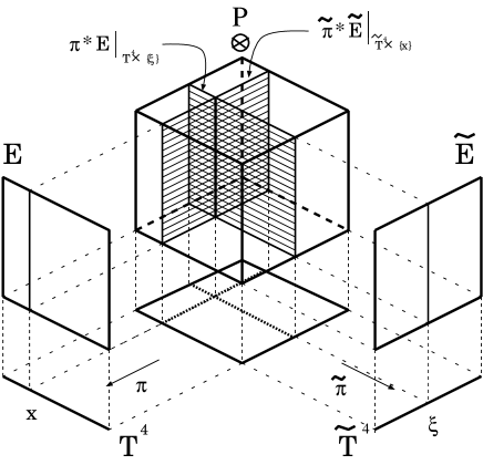
Figure 1: The stage of the Nahm transformation

The $U(k)$ gauge potential $\widetilde{A}$ is expressed by using the Dirac zero modes as

$$\widetilde{A}_{\mu}^{pq}(\xi)=\int_{T^{4}}d^{4}x~{}\psi^{p\dagger}_{\xi}(x)\frac{\partial}{\partial\xi^{\mu}}\psi^{q}_{\xi}(x)$$ (3.16)

where $\psi_{\xi}^{p}~{}(p=1,2,\ldots,k)$ are the normalized Dirac zero-modes.

$$\bar{{\cal D}}[A_{\xi}]\psi_{\xi}^{p}(x)=0,~{}~{}\int_{T^{4}}d^{4}x~{}\psi^{p\dagger}_{\xi}(x)\psi^{q}_{\xi}(x)=\delta^{pq}.$$ (3.17)

The 2nd Chern number of $\widetilde{E}$ turns out to be $N$ [7, 49]. Thus we obtain the $U(k)$ vector bundle $\widetilde{E}\rightarrow\widetilde{T}^{4}$ with $c_{2}(\widetilde{E})=N$ and the $U(k)$ gauge potential $\widetilde{A}$ on $\widetilde{E}$. This gives the Nahm transformation ${\cal N}:(E,A)\mapsto(\widetilde{E},\widetilde{A})$.

$$\begin{array}[]{ccccccc}{}\hfil&{}\hfil&{}\hfil&{}\hfil&\pi^{*}E\otimes{\cal P}&{}\hfil&{}\hfil\\ {}\hfil&{}\hfil&{}\hfil&{}\hfil&\downarrow&{}\hfil&{}\hfil\\ {}\hfil&{}\hfil&E&{}\hfil&T^{4}\times\widetilde{T}^{4}&{}\hfil&\widetilde{E}\\ {}\hfil&{}\hfil&\downarrow&\stackrel{{\scriptstyle\pi}}{{\swarrow}}&{}\hfil&\stackrel{{\scriptstyle\tilde{\pi}}}{{\searrow}}&\downarrow\\ {}\hfil&{}\hfil&T^{4}&{}\hfil&{}\hfil&{}\hfil&\widetilde{T}^{4}\end{array}$$

The inverse transformation is carried out by following the same procedure. Let $\widetilde{E}\rightarrow\widetilde{T}^{4}$ be a $U(k)$ vector bundle with $c_{2}(\widetilde{E})=N$ and $\widetilde{A}$ be a $U(k)$ gauge potential on $\widetilde{E}$. We regard the slice of the tensor product bundle $\widetilde{\pi}^{*}\widetilde{E}\otimes{\cal P}$ along $\{x\}\times\widetilde{T}^{4}$ as a $U(k)$ vector bundle over $\widetilde{T}^{4}$ equipped with the gauge potential $\widetilde{A}_{x}=\widetilde{A}\otimes 1_{[1]}-1_{[k]}\otimes ix^{\mu}d\xi_{\mu}$. The field strength $\widetilde{F}_{x}$ of $\widetilde{A}_{x}$ equals to $\widetilde{F}$ of $\widetilde{A}$. The Dirac operator acting on the sections $\Gamma(\widetilde{T}^{4},\widetilde{S}^{\pm}\otimes\pi^{*}\widetilde{E}\otimes{\cal P}|_{\{x\}\times\widetilde{T}^{4}})$ takes the form

$$\widetilde{{\cal D}}{[\widetilde{A}_{x}]} = e_{\mu}\otimes(\widetilde{\partial}^{\mu}+\widetilde{A}^{\mu}-ix^{\mu}),$$

$$\widetilde{\bar{{\cal D}}}{[\widetilde{A}_{x}]} = \bar{e}_{\mu}\otimes(\widetilde{\partial}^{\mu}+\widetilde{A}^{\mu}-ix^{\mu}).$$ (3.19)

By using the zero modes of $\widetilde{\bar{{\cal D}}}{[\widetilde{A}_{x}]}$, consisting of $N$ normalizable ones, we obtain a $U(N)$ vector bundle $E\rightarrow T^{4}$ with $c_{2}(E)=k$ and a $U(N)$ gauge potential $A$ on $E$. This gives the inverse Nahm transformation $\widetilde{{\cal N}}:(\widetilde{E},\widetilde{A})\mapsto(E,A)$.

$$\begin{array}[]{ccccccc}{}\hfil&{}\hfil&{}\hfil&{}\hfil&\tilde{\pi}^{*}\widetilde{E}\otimes{\cal P}&{}\hfil&{}\hfil\\ {}\hfil&{}\hfil&{}\hfil&{}\hfil&\downarrow&{}\hfil&{}\hfil\\ {}\hfil&{}\hfil&E&{}\hfil&T^{4}\times\widetilde{T}^{4}&{}\hfil&\widetilde{E}\\ {}\hfil&{}\hfil&\downarrow&\stackrel{{\scriptstyle\pi}}{{\swarrow}}&{}\hfil&\stackrel{{\scriptstyle\tilde{\pi}}}{{\searrow}}&\downarrow\\ {}\hfil&{}\hfil&T^{4}&{}\hfil&{}\hfil&{}\hfil&\widetilde{T}^{4}\end{array}$$

It can be shown ${\cal N}\widetilde{{\cal N}}=\widetilde{{\cal N}}{\cal N}=id.$ [7, 49]. Thus, eventually, $\widetilde{{\cal N}}$ turns out to be the inverse of ${\cal N}$. The Nahm duality is summarized in the following dictionary.

$$\begin{array}[]{ccc}G=U(N)&{}\hfil&\widetilde{G}=U(k)\\ k\mbox{-instanton on }T^{4}&\stackrel{{\scriptstyle 1~{}:~{}1}}{{\longleftrightarrow}}&N\mbox{-instanton on }\widetilde{T}^{4}\\ ~{}(\mbox{coord. }x^{\mu})&{}\hfil&~{}(\mbox{coord. }\xi^{\mu})\\ {}\hfil&\mbox{massless Dirac eq.}&{}\hfil\\ {}\hfil&\bar{{\cal D}}\psi=0&{}\hfil\\ \mbox{instanton}~{}:~{}A_{\mu[N]}&\stackrel{{\scriptstyle k\mbox{ solutions}:~{}\psi({\xi},x)}}{{\longrightarrow}}&\displaystyle\widetilde{A}_{\mu[k]}=\int_{T^{4}}d^{4}x~{}\psi^{\dagger}\frac{\partial}{\partial\xi^{\mu}}\psi\\ {}\hfil&{}\hfil&{}\hfil\\ {}\hfil&\mbox{massless Dirac eq.}&{}\hfil\\ {}\hfil&\widetilde{\bar{{\cal D}}}v=0&{}\hfil\\ \displaystyle A_{\mu[N]}=\int_{\widetilde{T}^{4}}d^{4}\xi~{}v^{\dagger}\frac{\partial}{\partial x^{\mu}}v&\stackrel{{\scriptstyle N\mbox{ solutions}:~{}v(x,\xi)}}{{\longleftarrow}}&\mbox{instanton}~{}:~{}\widetilde{A}_{\mu[k]}\\ \end{array}$$

3.3 A Derivation of the ADHM construction from the Nahm transformation

We can understand the duality in the ADHM/Nahm construction in some limit of the Nahm duality.

• Taking all four radii of the four-torus infinity $\Rightarrow$ ADHM construction of instantons

  Then the radii of the dual torus become zero. Hence the dual torus shrinks into one point and derivatives become meaningless because derivatives measure difference between two points. As the result, all derivatives in the dual ASD equation and the dual massless Dirac equation drop out and the differential equations becomes matrix equations. This naively yields the ADHM duality: one-to-one correspondence between the moduli space of the ASD equations on $\mathbb{R}^{4}$ (=infinite-size torus) and the moduli space of the matrix equations. For more detailed discussion, see [55].

• Taking three radii infinity and the other radius zero $\Rightarrow$ Nahm construction of monopoles

4 ADHM Construction of Instantons

In this section, we explain the ADHM construction of instantons on noncommutative Euclidean $\mathbb{R}^{4}$. Let $B_{1}$ and $B_{2}$ be $k\times k$ complex matrices, and $I$ and $J$ be $k\times N$ and $N\times k$ complex matrices. The ADHM data for noncommutative $U(N)$ $k$-instantons are quadruple matrices $B_{1},B_{2},I$ and $J$ which satisfy the noncommutative version of the ADHM equation.

$$\mu_{\mathbb{R}}\equiv{[B_{1},B_{1}^{\dagger}]}+[B_{2},B_{2}^{\dagger}]+II^{\dagger}-J^{\dagger}J=\zeta, \mu_{\mathbb{C}}\equiv{[B_{1},B_{2}]}+IJ=0,$$ (4.1)

where $\zeta\equiv-[\hat{z}_{1},\hat{\bar{z}}_{1}]-[\hat{z}_{2},\hat{\bar{z}}_{2}]=-2(\theta_{1}+\theta_{2})$ in the first equation of (4.1) is a non-negative constant originated in the noncommutativity (2.1). In the case that $\theta^{\mu\nu}$ is anti-self-dual, $\zeta$ vanishes and the noncommutative ADHM equation (4.1) coincides with the commutative ADHM equation. With the ADHM data, we associate “0-dimensional Dirac equation”

$$\hat{\nabla}^{\dagger}\cdot\hat{V}=0,~{}~{}~{}\hat{\nabla}(x)=\left(\begin{array}[]{cc}I^{\dagger}&J\\ \hat{\bar{z}}_{2}-B_{2}^{\dagger}&~{}-(\hat{z}_{1}-B_{1})\\ \hat{\bar{z}}_{1}-B_{1}^{\dagger}&~{}\hat{z}_{2}-B_{2}\end{array}\right).$$ (4.5)

The solution $\hat{V}$ of equation (4.5) is an $(N+2k)\times N$ matrix.

In the noncommutative case, we need to take care about the existence of zero-modes of $\hat{V}$. We may normalize $\hat{V}$ so that

$$\hat{V}^{\dagger}\cdot\hat{V}=1_{N}.$$ (4.6)

By using the normalized $\hat{V}$, we finally obtain the corresponding instanton solution as

$$\hat{A}_{\mu}=\hat{V}^{\dagger}\cdot\partial_{\mu}\hat{V}.$$ (4.7)

Actually, owing to the construction similar to the commutative case, the gauge potential (4.7) turns out to satisfy the noncommutative anti-self-dual Yang-Mills equation (2.24). The instanton number is computed to be $k$.

We will focus mainly on the case of $(N,k)=(2,1)$ in the subsequent discussions. For further reviews on noncommutative instantons, see [17, 21, 32, 34, 41, 48].

4.1 ADHM Construction of Commutative Instantons

To argue the ADHM construction of noncommutative instantons, it is convenient to recall the commutative case. We illustrate the case by the Belavin-Polyakov-Schwartz-Tyupkin (BPST) instanton [6], that is, a $SU(2)$ 1-instanton on commutative Euclidean $\mathbb{R}^{4}$.

In the case of $k=1$, $B_{1}$ and $B_{2}$ can be chosen as arbitrary complex numbers. The ADHM equation is then solved by using a real non-negative number $\rho$ as

$$B_{1}=\alpha_{1},~{}B_{2}=\alpha_{2},~{}I=(\rho,\,0),~{}J=\left(\begin{array}[]{c}0\\[-2.84526pt] \rho\end{array}\right),~{}~{}~{}\alpha_{1,2}\in\mathbb{C},~{}\rho\in\mathbb{R}_{\geq 0}.$$ (4.10)

The complex numbers $\alpha_{i=1,2}$ describe the position of the instanton. They can be always made zero by the coordinate shift $z_{i}\rightarrow z_{i}+\alpha_{i}$ in the Dirac equation. We will put $\alpha_{1}=\alpha_{2}=0$, without any loss. The normalized solution of the Dirac equation (4.5) takes the form

$$V=\frac{1}{\sqrt{\phi}}\left(\begin{array}[]{cc}z_{2}&z_{1}\\ -\bar{z}_{1}&\bar{z}_{2}\\ -\rho&0\\ 0&-\rho\\ \end{array}\right),~{}~{}~{}\phi=r^{2}+\rho^{2},~{}~{}r=\sqrt{{z}_{1}\bar{z}_{1}+{z}_{2}\bar{z}_{2}}.$$ (4.15)

The corresponding instanton solution $\displaystyle A_{\mu}=V^{\dagger}\partial_{\mu}V$ reads

$$A_{\mu}=\frac{r^{2}}{r^{2}+\rho^{2}}g^{-1}\partial_{\mu}g,~{}~{}~{}g=\frac{1}{r}\left(\begin{array}[]{cc}z_{2}&z_{1}\\ -\bar{z}_{1}&\bar{z}_{2}\end{array}\right).$$ (4.18)

The field strength is computed to be

$$F_{\mu\nu}=\frac{2i\rho^{2}}{(r^{2}+\rho^{2})^{2}}\eta_{{\mu\nu}},$$ (4.19)

where $\eta_{\mu\nu}$ is a $2\times 2$ matrix obtained by contracting ’t Hooft’s anti-self-dual eta symbol with the Pauli matrices as $\eta_{\mu\nu}=\eta^{a}_{\mu\nu}\sigma_{a}$. This is exactly the BPST instanton solution [6]. $\rho$ describes the size of the instanton.

In the limit $\rho\rightarrow 0$, the field strength (4.19) concentrates at the origin and becomes singular. In the framed instanton moduli space ${\cal{M}}$, it is a singularity called the small instanton singularity. The moduli space is depicted in Fig. 2, where the distributions of $\mbox{Tr}F_{{\mu\nu}}F^{{\mu\nu}}$ for the cases of $\rho\neq 0$ and $\rho=0$ are illustrated on the right-hand side.

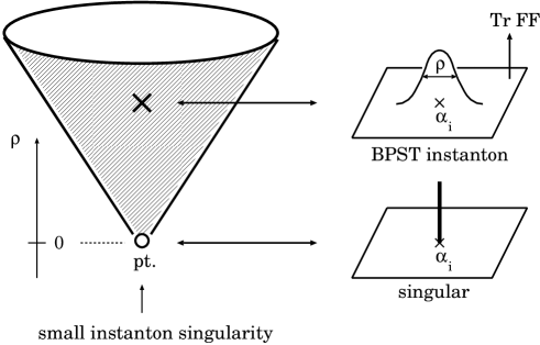
Figure 2: Instanton moduli space and configurations of the BPST instanton ($\zeta=0$)

4.2 ADHM Construction of NC instantons ($\zeta>0$)

Moduli space of noncommutative instantons depends on the constant $\zeta$ [38, 39]. When $\zeta=0$, the moduli space coincides with that of commutative instantons and contains the small instanton singularities. On the other hand, when $\zeta>0$, such singularities disappear and are replaced by a new class of smooth instantons, $U(1)$ instantons. In this subsection, we examine the case of $\zeta>0$. Let $\theta_{1}=\theta_{2}=-\zeta/4$. We construct a noncommutative instanton located at the origin, and observe how the new class of instantons appears on the noncommutative space, replacing the small instanton singularity.

4.2.1 NC $U(1)$ instantons ($\zeta>0$)

It is convenient to consider first the case of noncommutative $U(1)$ instantons. The ADHM data for a noncommutative $U(1)$ $1$-instanton is

$$B_{1}=B_{2}=0,~{}I=\sqrt{\zeta},~{}J=0.$$ (4.20)

The Dirac equation (4.5) reads

$$\hat{\nabla}^{\dagger}\cdot\hat{V}=\left(\begin{array}[]{ccc}\sqrt{\zeta}&\hat{z}_{2}&\hat{z}_{1}\\ 0&-\hat{\bar{z}}_{1}&\hat{\bar{z}}_{2}\end{array}\right)\cdot\hat{V}=0.$$ (4.23)

The following form of $\hat{V}$ gives a solution of (4.23).

$$\hat{V}_{1}=\left(\begin{array}[]{cc}\hat{z}_{1}\hat{\bar{z}}_{1}+\hat{z}_{2}\hat{\bar{z}}_{2}\\ -\sqrt{\zeta}\hat{\bar{z}}_{2}\\ -\sqrt{\zeta}\hat{\bar{z}}_{1}\end{array}\right),$$ (4.27)

where $\hat{V}_{1}$ is an operator acting on the Fock space $\cal{H}$. Since $2(\theta_{1}+\theta_{2})=-\zeta<0$, the commutation relations (2.21) imply that at least either coordinates $\hat{\bar{z}}_{1}$ or $\hat{\bar{z}}_{2}$ is the annihilation operator. Actually, at present, we put $\theta_{1}=\theta_{2}=-\zeta/4$. This means that both the coordinates are the annihilation operators. $\hat{V}_{1}$ has the kernel, an operator zero-mode $|0,0\rangle$. Thus, it can not provide a normalized solution to satisfy the condition (4.6).

K. Furuuchi [15] shows that $\hat{V}_{1}$ yields a smooth anti-self-dual instanton solution on the subspace ${\cal H}_{1}\equiv{\cal H}\setminus\mathbb{C}|0,0\rangle$. Using the shift operator, he also discussed that it can be modified to satisfy the condition (4.6) on ${\cal H}$. Let $\hat{U}_{1}$ be a shift operator of the form

$$\hat{U}_{1}=\sum_{n_{1}=1}^{+\infty}\sum_{n_{2}=0}^{+\infty}|n_{1},n_{2}\rangle\langle n_{1},n_{2}|+\sum_{n_{2}=0}^{+\infty}|0,n_{2}\rangle\langle 0,n_{2}+1|.$$ (4.28)

It satisfies $\hat{U}_{1}\hat{U}_{1}^{\dagger}=1$ and $\hat{U}_{1}^{\dagger}\hat{U}_{1}=1-\hat{P}_{1}$, where $\hat{P}_{1}=|0,0\rangle\langle 0,0|$ is the projection operator to the kernel. The modification reads [16]

$$\hat{V}=\hat{V}_{1}\hat{{\beta}}_{1}\hat{U}_{1}^{\dagger}, \hat{{\beta}}_{1}\equiv(1-\hat{P}_{1})\left(\hat{V}_{1}^{\dagger}\hat{V}_{1}\right)^{-\frac{1}{2}}(1-\hat{P}_{1}).$$ (4.29)

The modified operator (4.29) satisfies $\hat{V}^{\dagger}\hat{V}=1$ on ${\cal H}$. This can be seen by a direct computation of $\hat{V}^{\dagger}\hat{V}$ using (4.27) and (4.28) together with $\hat{\beta}_{1}$ in the following form.

$$\hat{{\beta}}_{1}=\frac{2}{\zeta}\sum_{(n_{1},n_{2})\neq(0,0)}\frac{|n_{1},n_{2}\rangle\langle n_{1},n_{2}|}{\sqrt{(n_{1}+n_{2})(n_{1}+n_{2}+2)}}.$$ (4.30)

Thus the obtained normalized solution (4.29) gives in the sequel a smooth anti-self-dual instanton on ${\cal H}$ with the instanton number equal to $1$.

4.2.2 NC $U(2)$ instantons ($\zeta>0$)

Noncommutative BPST solution is a noncommutative version of the BPST instanton and can be also obtained by the ADHM construction. The ADHM data is

$$B_{1}=B_{2}=0,~{}~{}~{}I=(\sqrt{\rho^{2}+\zeta},0),~{}~{}~{}J=\left(\begin{array}[]{c}0\\ \rho\end{array}\right).$$ (4.33)

Compared with the commutative case (4.10), $I$ in the ADHM data is deformed by $\zeta$. This implies that the size of instanton is not less than $\sqrt{\zeta}$.

Normalized solution of the Dirac equation can be found by Furuuchi’s approach [16, 17]. We first see that the following form of $\hat{V}$ is a solution of the Dirac equation.

$$\hat{V}_{1}=\Bigl{(}\hat{V}_{1}^{(1)},\,\hat{V}_{1}^{(2)}\Bigr{)}$$ (4.34)

where

$$\hat{V}_{1}^{(1)}=\left(\begin{array}[]{cc}\hat{z}_{1}\hat{\bar{z}}_{1}+\hat{z}_{2}\hat{\bar{z}}_{2}\\ 0\\ -\sqrt{\rho^{2}+\zeta}\,\hat{\bar{z}}_{2}\\ -\sqrt{\rho^{2}+\zeta}\,\hat{\bar{z}}_{1}\end{array}\right), \hat{V}_{1}^{(2)}=\left(\begin{array}[]{cc}0\\ \hat{z}_{1}\hat{\bar{z}}_{1}+\hat{z}_{2}\hat{\bar{z}}_{2}+\zeta\\ \rho\,\hat{z}_{1}\\ -\rho\,\hat{z}_{2}\end{array}\right).$$ (4.43)

Apparently, $\hat{V}_{1}^{(1)}$ has the same kernel as (4.27), while $\hat{V}_{1}^{(2)}$ is injective. To obtain a normalized solution from (4.34), we introduce the shift operator $\hat{U}_{1}$ which satisfies

$$\hat{U}_{1}\hat{U}_{1}^{\dagger}=1, \hat{U}_{1}^{\dagger}\hat{U}_{1}=1-\left(\begin{array}[]{cc}\hat{P}_{1}&0\\ 0&0\end{array}\right).$$ (4.46)

It is actually given by

$$\hat{U}_{1}=\sqrt{\frac{2}{\zeta}}\left(\begin{array}[]{cc}\hat{\bar{z}}_{2}&-\hat{z}_{1}\\ \hat{\bar{z}}_{1}&\hat{z}_{2}\end{array}\right)\sum_{n_{1}=0}^{+\infty}\sum_{n_{2}=0}^{+\infty}\frac{|n_{1},n_{2}\rangle\langle n_{1},n_{2}|}{\sqrt{n_{1}+n_{2}+1}}.$$ (4.49)

Combining these operators, the normalized solution $\hat{V}=(\hat{V}^{(1)},\hat{V}^{(2)})$ is obtained in the following form.

$$\hat{V}=\hat{V}_{1}\cdot\left(\begin{array}[]{cc}\hat{\beta}_{1}^{(1)}&0\\[-2.84526pt] 0&\hat{\beta}_{1}^{(2)}\end{array}\right)\cdot\hat{U}_{1}^{\dagger},$$ (4.52)

where

$${\displaystyle\hat{\beta}_{1}^{(1)}=\frac{2}{\zeta}\sum_{(n_{1},n_{2})\neq(0,0)}\frac{|n_{1},n_{2}\rangle\langle n_{1},n_{2}|}{\sqrt{(n_{1}+n_{2})(n_{1}+n_{2}+2+\frac{2\rho^{2}}{\zeta})}}},$$

$${\displaystyle\hat{\beta}_{1}^{(2)}=\frac{2}{\zeta}\sum_{n_{1}=0}^{+\infty}\sum_{n_{2}=0}^{+\infty}\frac{|n_{1},n_{2}\rangle\langle n_{1},n_{2}|}{\sqrt{(n_{1}+n_{2}+2)(n_{1}+n_{2}+2+\frac{2\rho^{2}}{\zeta})}}}.$$ (4.53)

The normalized solution (4.52) turns out to give a smooth anti-self-dual instanton on ${\cal H}$ with the instanton number equal to $1$, that is, the noncommutative BPST instanton. It keeps to be smooth in the limit $\rho\rightarrow 0$ and becomes the $U(1)$ instanton. This is because $\hat{V}^{(2)}$ decouples at this limit and does not contribute to the field strength. (See Fig. 3.)

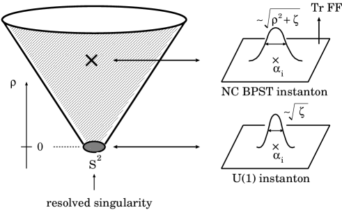
Figure 3: Instanton moduli space and the configuration of the NC BPST instanton ($\zeta>0$)

The BPST instantons on commutative and noncommutative spaces are summarized in the following table.

BPST instanton	$(N,k)=(2,1)$	NC BPST instanton
$\mu_{\mathbb{R}}=0,~{}\mu_{\mathbb{C}}=0$	ADHM equation	$\mu_{\mathbb{R}}=\zeta>0,~{}\mu_{\mathbb{C}}=0$
$B_{1,2}=\alpha_{1,2},$	ADHM data	$B_{1,2}=\alpha_{1,2},$
$I=(\rho,0),J^{t}=(0,\rho)$		$I=(\sqrt{\rho^{2}+\zeta},0),J^{t}=(0,\rho)$
$\mathbb{R}^{4}\times$ orbifold $\mathbb{C}^{2}/\mathbb{Z}_{2}$	moduli space	$\mathbb{R}^{4}\times$ Eguchi-Hanson $\widetilde{\mathbb{C}^{2}/\mathbb{Z}_{2}}$
(singular)		(regular)
$F_{{\mu\nu}}\rightarrow$ (singular)	zero-size limit	$F_{{\mu\nu}}\rightarrow$ $U(1)$ instanton (regular)

4.3 ADHM Construction of NC instantons ($\zeta=0$)

Finally we discuss the ADHM construction of noncommutative instantons at the special value, $\zeta=0$, where the noncommutative parameter is anti-self-dual and satisfies in the canonical form, $\theta_{1}=-\theta_{2}\neq 0$. We set $\theta_{1}=-\theta_{2}\equiv\theta>0$. Hence the coordinate $\hat{\bar{z}}_{1}$ is now the creation operator, while $\hat{\bar{z}}_{2}$ is still the annihilation operator. We consider the instantons at the origin.

4.3.1 NC $U(1)$ instantons ($\zeta=0$)

The instanton moduli space is the same as the commutative one and contains the small instanton singularities. Let us first examine the $U(1)$ instanton that gives the small instanton singularity. The ADHM data is trivial.

$$B_{1,2}=0,~{}I=0,~{}J=0.$$ (4.54)

The normalized solution of the Dirac equation (4.5) is given [20] by

$$\hat{V}=\left(\begin{array}[]{c}\hat{U}_{1}\\ 0\\ \hat{P}_{1}\end{array}\right),$$ (4.58)

where $\hat{U}_{1}$ is the shift operator in (4.28). The normalization condition (4.6) can be seen as $\displaystyle\hat{V}^{\dagger}\hat{V}=\hat{U}_{1}^{\dagger}\hat{U}_{1}+\hat{P}_{1}=(1-\hat{P}_{1})+\hat{P}_{1}=1$. Operators of covariant derivative and field strength take the following forms.

$$\hat{D}_{z_{i}}=\hat{U}_{1}^{\dagger}\hat{\partial}_{z_{i}}\hat{U}_{1},~{}~{}~{}~{}\hat{F}_{z_{1}\bar{z}_{1}}=-\hat{F}_{z_{2}\bar{z}_{2}}=\frac{1}{2\theta}\hat{P}_{1}.$$ (4.59)

The second Chern class $(-1/16\pi^{2})\mbox{Tr}\hat{F}_{{\mu\nu}}\hat{F}^{{\mu\nu}}$ is easily computed to be $(2\pi\theta)^{-2}\hat{P}_{1}$. It is converted to the Gaussian distribution $(\pi\theta)^{-2}\exp(-r^{2}/\theta)$ in the star-product formalism by the inverse Weyl-transformation. The instanton number is found to be $1$.

This type of exact solutions is first given in [2] and plays important roles in string theory (e.g. [27]).

4.3.2 NC $U(2)$ instantons ($\zeta=0$)

When $\zeta=0$, the ADHM construction of noncommutative BPST instantons is simpler than the previous case. The ADHM data is the same as the commutative one (4.10).

$$B_{1,2}=0,~{}~{}~{}I=(\rho,0),~{}~{}~{}J=\left(\begin{array}[]{c}0\\ \rho\end{array}\right).$$ (4.62)

The normalized solution of the Dirac equation (4.5) is [18]:

$$\hat{V} = (\hat{V}^{(1)},\hat{V}^{(2)}),$$ (4.63)

$$\hat{V}^{(1)} = \left(\begin{array}[]{c}\hat{z}_{2}\\ -\hat{\bar{z}}_{1}\\ -\rho\\ 0\end{array}\right)\sum_{n_{1},n_{2}}\frac{|n_{1},n_{2}\rangle\langle n_{1},n_{2}|}{\sqrt{2\theta(n_{1}+n_{2}+1)+\rho^{2}}},~{}\hat{V}^{(2)}=\left(\begin{array}[]{c}\hat{z}_{1}\\ \hat{\bar{z}}_{2}\\ 0\\ -\rho\end{array}\right)\sum_{n_{1},n_{2}}\frac{|n_{1},n_{2}\rangle\langle n_{1},n_{2}|}{\sqrt{2\theta(n_{1}+n_{2})+\rho^{2}}}.$$ (4.72)

This possesses similar structure as the commutative one (4.15) ($r^{2}\leftrightarrow 2\theta(n_{1}+n_{2})$). The solution (4.63) gives a smooth anti-self-dual instanton with the instanton number $1$. In the limit $\rho\rightarrow 0$, this reduces to that of the $U(1)$ 1-instanton (4.58).

5 Conclusion and Discussion

In this paper, we constructed exact noncommutative instanton solutions by the ADHM procedure. We further prove one-to-one correspondence between the moduli space of the $U(N)$ $k$-instantons and the moduli space of the ADHM data labeled by $(N,k)$ [26]. In the proof, we apply Furuuchi’s observation and several properties on noncommutative field theory (especially NC-deformed index theorem by Maeda and Sako [35]) to all the other ingredients of the ADHM construction and prove the existence of them in the operator sense. As a result, we obtain the following formula (a noncommutative version of the Corrigan-Goddard-Osborn-Templeton or Osborn formula [11, 45])

$$\int d^{4}x{\mbox{ Tr}}_{N}(F_{\mu\nu}\star F^{\mu\nu})=-\int d^{4}x\partial^{2}\partial_{\mu}({\mbox{Tr}}_{k}f^{-1}\star\partial^{\mu}f),~{}f:=(\nabla^{\dagger}\star\nabla)^{-1}.$$ (5.1)

By using this formula and the asymptotic behavior of $f\simeq|x|^{-2}1_{k}$, the instanton number (the second Chern number) is computed after surface integration as

$$\frac{-1}{16\pi^{2}}\int d^{4}x{\mbox{ Tr}}_{N}(F_{\mu\nu}\star F^{\mu\nu})={\mbox{Tr}}_{k}1_{k}=k.$$

This directly shows an origin of the instanton number from the language of the ADHM data. (For other discussion on the instanton number, see e.g. [9, 17, 29, 47, 53, 54].) Detailed proofs and other results are seen in our paper [26].

Acknowledgments

The authors thank the Yukawa Institute for Theoretical Physics at Kyoto University. Discussions during the YITP workshop on “Field Theory and String Theory” (YITP-W-12-05) were useful to complete this work. The authors are also grateful to A. Sako for fruitful discussion. MH is supported in part by the Daiko Foundation, the Toyoaki Scholarship Foundation, and the Grant-in-Aid for Young Scientists (#23740182). TN is supported in part by the Grant-in-Aid for Scientific Research No. 24540223.

References

- [1]
- [2] M. Aganagic, R. Gopakumar, S. Minwalla and A. Strominger, “Unstable solitons in noncommutative gauge theory,” JHEP 0104 (2001) 001 [hep-th/0009142].
- [3] T. Asakawa, U. Carow-Watamura, Y. Teshima and S. Watamura, “Boundary state analysis on the equivalence of T-duality and Nahm transformation in superstring theory,” Prog. Theor. Phys. 127 (2012) 665 [arXiv:1201.0125].
- [4] M. F. Atiyah, N. J. Hitchin, V. G. Drinfeld and Y. I. Manin, “Construction of instantons,” Phys. Lett. A 65 (1978) 185.
- [5] C. Bartocci, U. Bruzzo and D. H. Ruipérez, Fourier-Mukai and Nahm Transforms in Geometry and Mathematical Physics (Birkhäuser, 2009) [ISBN/978-0-8176-4663-9].
- [6] A. A. Belavin, A. M. Polyakov, A. S. Schwartz and Y. S. Tyupkin, “Pseudoparticle solutions of the Yang-Mills equations,” Phys. Lett. B 59 (1975) 85.
- [7] P. J. Braam and P. van Baal, “Nahm’s Transformation For Instantons,” Commun. Math. Phys. 122 (1989) 267.
- [8] C. -S. Chu, “Non-commutative geometry from strings,” hep-th/0502167.
- [9] C. S. Chu, V. V. Khoze and G. Travaglini, “Notes on noncommutative instantons,” Nucl. Phys. B 621 (2002) 101 [hep-th/0108007].
- [10] E. Corrigan and P. Goddard, “Construction of instanton and monopole solutions and reciprocity,” Annals Phys. 154 (1984) 253.
- [11] E. Corrigan, P. Goddard, H. Osborn and S. Templeton, “Zeta function regularization and multi-instanton determinants,” Nucl. Phys. B 159 (1979) 469.
- [12] S. K. Donaldson and P. B. Kronheimer, The Geometry of Four-Manifolds (Oxford UP, 1990) [ISBN/0-19-850269-9].
- [13] N. Dorey, T. J. Hollowood, V. V. Khoze and M. P. Mattis, “The calculus of many instantons,” Phys. Rept. 371 (2002) 231 [hep-th/0206063].
- [14] M. R. Douglas and N. A. Nekrasov, “Noncommutative field theory,” Rev. Mod. Phys. 73 (2002) 977 [hep-th/0106048].
- [15] K. Furuuchi, “Instantons on noncommutative and projection operators,” Prog. Theor. Phys. 103 (2000) 1043 [hep-th/9912047].
- [16] K. Furuuchi, “Equivalence of projections as gauge equivalence on noncommutative space,” Commun. Math. Phys. 217 (2001) 579 [hep-th/0005199].
- [17] K. Furuuchi, “Topological charge of instantons on noncommutative ,” hep-th/0010006.
- [18] K. Furuuchi, “ in noncommutative Yang-Mills,” JHEP 0103 (2001) 033 [hep-th/0010119].
- [19] C. R. Gilson, M. Hamanaka and J. J. C. Nimmo, “Bäcklund Transformations and the Atiyah-Ward ansatz for Noncommutative Anti-Self-Dual Yang-Mills Equations,” Proc. Roy. Soc. Lond. A 465 (2009) 2613 [arXiv:0812.1222].
- [20] M. Hamanaka, “Atiyah-Drinfeld-Hitchin-Manin and Nahm Constructions of localized solitons in noncommutative gauge theories,” Phys. Rev. D 65 (2002) 085022 [hep-th/0109070].
- [21] M. Hamanaka, “Noncommutative solitons and D-branes,” Ph.D thesis (University of Tokyo, 2003) hep-th/0303256.
- [22] M. Hamanaka, “Noncommutative Ward’s conjecture and integrable systems,” Nucl. Phys. B 741 (2006) 368 [hep-th/0601209].
- [23] M. Hamanaka and H. Kajiura, “Gauge fields on tori and T duality,” Phys. Lett. B 551 (2003) 360 [hep-th/0208059].
- [24] M. Hamanaka and T. Nakatsu, “Noncommutative instantons revisited,” J. Phys. Conf. Ser. 411 (2013) 012016.
- [25] M. Hamanaka and T. Nakatsu, “Exact construction of noncommutative instantons,” Frontiers of Mathematics in China 8 (2013) 1031.
- [26] M. Hamanaka and T. Nakatsu, “ADHM construction and group actions for noncommutative instantons,” in preparation.
- [27] J. A. Harvey, “Komaba lectures on noncommutative solitons and D-branes,” [hep-th/0102076].
- [28] K. Hori, “D-branes, T duality, and index theory,” Adv. Theor. Math. Phys. 3 (1999) 281 [hep-th/9902102].
- [29] T. Ishikawa, S. I. Kuroki and A. Sako, “Instanton number calculus on noncommutative ,” JHEP 0208 (2002) 028 [hep-th/0201196].
- [30] M. Jardim, “A survey on Nahm transform,” J. Geom. Phys. 52 313 [math/0309305]
- [31] A. Konechny and A. Schwarz, “Introduction to M(atrix) theory and noncommutative geometry,” Phys. Rept. 360 (2002) 353 [hep-th/0012145].
- [32] A. Konechny and A. Schwarz, “Introduction to M(atrix) theory and noncommutative geometry, II,” Phys. Rept. 360 (2002) 353 [hep-th/0107251].
- [33] P. B. Kronheimer and H. Nakajima, “Yang-Mills instantons on ALE gravitational instantons,” Math. Ann. 288 (1990) 263.
- [34] O. Lechtenfeld, “Noncommutative instantons and solitons,” Fortsch. Phys. 52, 596 (2004) [hep-th/0401158].
- [35] Y. Maeda and A. Sako, “Noncommutative Deformation of Spinor Zero Mode and ADHM Construction,” J. Math. Phys. 53 (2012) 022303 [arXiv:0910.3441].
- [36] L. J. Mason and N. M. Woodhouse, Integrability, Self-Duality, and Twistor Theory (Oxford UP, 1996) [ISBN/0-19-853498-1].
- [37] J. E. Moyal, “Quantum mechanics as a statistical theory,” Proc. Cambridge Phil. Soc. 45 (1949) 99.
- [38] H. Nakajima, “Resolutions of moduli spaces of ideal instantons on ,” in Topology, Geometry and Field Theory (World Sci., 1994) 129 [ISBN/981-02-1817-6].
- [39] H. Nakajima, Lectures on Hilbert Schemes of Points on Surfaces (AMS, 1999) [ISBN/0-8218-1956-9].
- [40] H. Nakajima and K. Yoshioka, “Instanton counting on blowup. 1.,” Invent. Math. 162 (2005) 313 [math/0306198].
- [41] N. A. Nekrasov, “Trieste lectures on solitons in noncommutative gauge theories,” hep-th/0011095.
- [42] N. A. Nekrasov, “Lectures on open strings, and noncommutative gauge fields,” [hep-th/0203109].
- [43] N. A. Nekrasov, “Seiberg-Witten prepotential from instanton counting,” Adv. Theor. Math. Phys. 7 (2004) 831. [hep-th/0206161].
- [44] N. Nekrasov and A. Schwarz, “Instantons on noncommutative , and (2,0) superconformal six dimensional theory,” Commun. Math. Phys. 198 (1998) 689 [hep-th/9802068].
- [45] H. Osborn, “Calculation of multi-instanton determinants,” Nucl. Phys. B 159 (1979) 497.
- [46] R. Penrose, “Twistor algebra,” J. Math. Phys. 8 (1967) 345–366.
- [47] A. Sako, “Instanton number of noncommutative gauge theory,” JHEP 04 (2003) 023 [hep-th/0209139].
- [48] F. A. Schaposnik, “Noncommutative solitons and instantons,” Braz. J. Phys. 34 (2004) 1349 [hep-th/0310202].
- [49] H. Schenk, “On A Generalized Fourier Transform Of Instantons Over Flat Tori,” Commun. Math. Phys. 116 (1988) 177.
- [50] N. Seiberg and E. Witten, “String theory and noncommutative geometry,” JHEP 9909 (1999) 032 [hep-th/9908142].
- [51] R. J. Szabo, “Quantum field theory on noncommutative spaces,” Phys. Rept. 378 (2003) 207 [hep-th/0109162].
- [52] K. Takasaki, “Anti-self-dual Yang-Mills equations on noncommutative spacetime,” J. Geom. Phys. 37 (2001) 291 [hep-th/0005194].
- [53] Y. Tian, “Topological charge of ADHM instanton on ,” Mod. Phys. Lett. A 19 (2004) 1315 [hep-th/0404128]
- [54] Y. Tian, C. J. Zhu and X. C. Song, “Topological charge of noncommutative ADHM instanton,” Mod. Phys. Lett. A 18 (2003) 1691 [hep-th/0211225]
- [55] P. van Baal, “Instanton moduli for ,” Nucl. Phys. Proc. Suppl. 49 (1996) 238 [hep-th/9512223].
- [56] R. S. Ward, “Integrable and solvable systems, and relations among them,” Phil. Trans. Roy. Soc. Lond. A 315 (1985) 451.
- [57] R. S. Ward and R. O. Wells, Twistor Geometry and Field Theory (Cambridge UP, 1990) [ISBN/0-521-42268-X].