Cosmological Constraints from the Anisotropic Clustering Analysis using BOSS DR9

Abstract

Our observations of the Universe are fundamentally anisotropic, with data from galaxies separated transverse to the line of sight coming from the same epoch while that from galaxies separated parallel to the line of sight coming from different times. Moreover, galaxy velocities along the line of sight change their redshift, giving redshift space distortions. We perform a full two-dimensional anisotropy analysis of galaxy clustering data, fitting in a substantially model independent manner the angular diameter distance $D_{A}$, Hubble parameter $H$, and growth rate $d\delta/d\ln a$ without assuming a dark energy model. The results demonstrate consistency with $\Lambda$CDM expansion and growth, hence also testing general relativity. We also point out the interpretation dependence of the effective redshift $z_{\rm eff}$, and its cosmological impact for next generation surveys.

I Introduction

Large volume galaxy redshift surveys are mapping large scale structure in the universe, measuring the three dimensional positions of millions of galaxies. This data teaches us not only the statistics of clustering but can be used to measure cosmic distances and growth, and constrain cosmological models. The third dimension of the data, the redshift, allows investigation of two effects: the role of cosmic expansion in distinguishing transverse and radial distances, and the role of peculiar velocities, measured through their induced redshift space anisotropy, as a probe of the cosmic structure growth rate.

Redshift space distortions (RSD) are induced by the large scale velocity flow of galaxies and are thus intimately connected to the growth rate of cosmic structure Kaiser:1987qv ; Hamilton (1998). Over the last 10 years, as the size of spectroscopic surveys has increased, this effect has been exploited, allowing testable predictions of general relativity on large scales Linder:2007nu ; Zhang:2007nk ; Jain:2007yk ; Wang:2007ht ; Guzzo:2008ac ; Song:2008qt ; Daniel:2010yt ; Song:2010rm ; Song:2010fg ; Reyes:2010tr ; Shafieloo:2012ms ; Reid:2012sw ; Yoo:2012vm .

Geometric distortions are induced by distances along and perpendicular to the line of sight being fundamentally different. Measuring the ratio of galaxy clustering radially to transversely provides a probe of this, called the Alcock-Paczynski effect Alcock:1979mp ; Padmanabhan:2008ag ; Gaztanaga:2008xz . Assuming the incorrect cosmological model for the coordinate transformation from redshift space to comoving Cartesian space leaves a residual geometric distortion. In observations the geometric effect is convolved with RSD Ballinger et al. (1996); Matsubara & Suto (1996), but the fixed physical scale of baryon acoustic oscillations (BAO) can alleviate this covariance Blake & Glazebrook (2003); Eisenstein et al. (2005).

The quantity and quality of data now allows the distinction of these effects through a full two dimensional (transverse-radial) analysis, rather than relying on a spherical average, a squashing (AP) ratio, or the lowest few multipoles of the clustering distribution. Following the method tested in Song:2013ejh , we fit the clustering correlation function in the transverse-radial plane, paying particular attention to the baryon acoustic oscillation (BAO) “ring of power” Hu:2003ti but using the full 2D clustering information.

Another advantage of this analysis is that it is carried out in a substantially model independent manner, without assuming LCDM or any other dark energy model. Instead we directly fit for the angular distance $D_{A}$, Hubble parameter $H$, and growth rate $G_{\Theta}\sim d\delta/d\ln a$ simultaneously from the 2D clustering statistics. Variation of each of these give distinct distortions of the clustering power isocontours, including the BAO ring of power. We analyze the SDSS DR9 galaxies in the BOSS CMASS Ahn:2012fh sample at an effective redshift of $z_{\rm eff}=0.57$.

This data has already given rise to several significant results in measuring cosmological distances, the first BAO detection in DR9 coming from Anderson:2013oza and Busca et al. (2013). This was followed by a more detailed study which found the distance ratio $D_{V}(z=0.57)=2094\pm 34$ Mpc Anderson:2013oza using typical correlation functions and power spectra analyses, where $D_{V}$ is a spherically averaged distance measure. Anisotropic analysis using “clustering wedges” placed tight constraints on the angular diameter distance and the Hubble constant: $D_{A}(z=0.57)/r_{s}(z_{d})=9.03\pm 0.21$ and $cz/(r_{s}(z_{d})H(z))=12.14\pm 0.43$ Sanchez:2013uxa ; Kazin:2013rxa . These measurements were confirmed by Reid:2012sw and Samushia et al. (2013) used the full shape of the monopole and quadrupole correlation functions to obtain estimates of $H(z)$, $D_{A}$ and the growth rate $d\delta/d\ln a$. This reduced set of cosmological observables was then used to place tight constraints on the cosmological parameters Samushia et al. (2013); Ross et al. (2013).

Angularly-averaged statistics, such as the multipoles mentioned above, successfully placed constraints on cosmological parameters. However, such statistics become complicated when one considers excluding data along the line-of-sight, e.g. that are much noisier than the data perpendicular to it Scoccimarro:2004tg or are difficult to model accurately because of velocity or nonlinear effects. It is thus meaningful to present the analysis of the correlation function in the transverse-radial plane, without angle averaging, as a complementary method.

Another advantage of using the full 2D correlation function is that one can easily distinguish between the geometric and velocity (RSD) effects, clarifying the physical interpretation. The 2D correlation function including the BAO scale was first analyzed by Okumura et al. (2008) but the analysis relied on linear theory Matsubara (2004). In Song:2013ejh we developed a formalism that predicts the correlation function in the 2D plane with nonlinear perturbation theory. Following the method tested in Song:2013ejh , we here fit the clustering correlation function in the transverse-radial plane to data.

The outline of this paper proceeds as follows. In Sec. II we briefly review the analysis method and treatment of nonlinearities and velocity effects. Section III details the measurement procedure including estimation of the covariance matrix. The results are presented in Sec. IV and the implications for cosmological models are discussed in Sec. V. We conclude in Sec. VI, with Appendix A exploring cautions regarding interpretation of $z_{\rm eff}$ at the accuracy of next generation surveys.

II Theoretical Model

The two–point correlation function of galaxy clustering, $\xi_{s}$, is described as a function of $\sigma$ and $\pi$ in the distant-observer limit, where $\sigma$ and $\pi$ are the transverse and the radial directions with respect to the observer. As mentioned in the Introduction, several effects give rise to anisotropy between these directions. In the linear density perturbation regime, RSD causes the clustering pattern to be squeezed along the line of sight (i.e. the $\pi$-direction), leading to an apparent enhancement of the amplitude of the observed correlation function. This is known as Kaiser effect Kaiser:1987qv . On the other hand, in the non–linear regime, the random virial motions of galaxies residing in halos introduce elongated clustering along the line of sight, which is dubbed the Finger of God effect (FoG). This dispersion effect has significant impact, and even on large scales (in linear theory), a simple description of $\xi_{s}(\sigma,\pi)$ using the Kaiser formula alone may not be adequate along the $\pi$ direction (e.g., Scoccimarro:2004tg ). In our previous paper, we combined this dispersion effect with the Kaiser formula to analyze two–dimensional anisotropy structure of DR7 catalogue Song:2010kq .

The precision of the updated DR9 clustering catalog is greatly improved. Due to this improvement, systematic uncertainties in accounting for the anisotropic clustering effects gain greater influence. Therefore we here employ improved distortion models to analyze the better precision maps. Due to a strong correlation between density and velocity fields, the mapping between real and redshift space is intrinsically non–linear Taruya:2010mx . In general, it appears as a not–closed iteration of polynomials for which a more elaborate description than simple factorized formulation needs to be used. However at large separation several leading polynomials dominate. In addition, we apply the non–linear correction terms using the resummed perturbation theory called RegPT Taruya:2007xy ; Taruya:2012ut . When restricting analysis to the quasi-linear regime, the result is the non–linear portions of the power spectra are better separated from the linear spectra, for which the assumption of perfect cross–correlation between density and velocity fields is verified.

In brief, we adopt the redshift-space power spectrum, $\tilde{P}(k,\mu)$, given in Ref. Taruya:2010mx , which can be recast as

$$\tilde{P}(k,\mu)=\sum_{n=0}^{4}\,Q_{2n}(k)\mu^{2n}\,G^{\rm FoG}(k\mu\sigma_{p})\,,$$ (1)

where $\sigma_{p}$ is a free parameter representing small scale velocity effects. Our previous analysis suggests that as long as we consider the weakly nonlinear scales, cosmological analysis can be made independently of the functional form of FoG effect. The functions $Q_{2n}$ are given in Song:2013ak .

From the power spectrum one can compute the correlation function by Fourier transform. The redshift-space correlation function $\xi(\sigma,\mu)$ is generally expanded as

$$\xi^{s}(\sigma,\pi) = \int\frac{d^{3}k}{(2\pi)^{3}}\tilde{P}(k,\mu)e^{i{\bf k}\cdot{\bf s}}$$ (2)

$$= \sum_{\ell\ {\rm even}}\xi_{\ell}(s){\cal P}_{\ell}(\nu)\,,$$

with ${\cal P}$ being the Legendre polynomials. Here, we define $\nu=\pi/s$ and $s=(\sigma^{2}+\pi^{2})^{1/2}$. The moments of correlation function are given in Song:2013ejh . Here we include the moments up to ${\ell}=6$, since the higher-order moments $\ell\geq 8$ are shown to contribute negligibly.

III Measurements

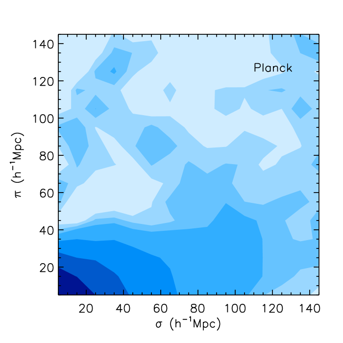
Figure 1: The measured 2D clustering correlation function $\xi(\sigma,\pi)$ is plotted, adopting early universe priors from WMAP9 (left) or Planck (right).

III.1 Data Sample

We use data from the Sloan Digital Sky Survey (SDSS; York et al., 2000), Data Release 9 (DR9). SDSS has mapped over one quarter of the sky in five photometric bands down to a limiting magnitude of $r\sim 22.5$. The photometric data is reduced and from it are selected targets for followup spectroscopy. The spectroscopic survey, known as the Baryon Oscillation Spectroscopic Survey (BOSS), is designed to obtain spectra for $\sim 1.5$ million galaxies over a 10,000 square degree footprint.

In an effort to control the evolution of galaxy bias over large redshift ranges the BOSS targets are selected in such a way as to have approximately constant stellar mass (CMASS). This is obtained using colour selections based on the passive galaxy template of (Maraston et al., 2009). The majority of CMASS galaxies are bright, central galaxies (in the halo model framework) and are thus highly biased ($b\sim 2$) (Nuza et al., 2013).

The CMASS sample CMASS is defined by

$$z > 0.4$$ (3)

$$17.5<i_{cmod} < 19.9$$

$$r_{mod}-i_{mod} < 2.0$$

$$d_{\perp} > 0.55$$

$$i_{fib2} < 21.5$$

$$i_{cmod} < 19.86+1.6(d_{\perp}-0.8)$$

$$i_{psf}-i_{mod} > 0.2+0.2(20.0-i_{mod})$$

$$z_{psf}-z_{mod} > 9.125-0.46z_{mod}\ ,$$

where the last two conditions provide a star-galaxy separator and $d_{\perp}$ is defined as (Cannon et al., 2006),

$$d_{\perp}=r_{mod}-i_{mod}-(g_{mod}-r_{mod})/8.0\ .$$ (4)

Each spectroscopically observed galaxy is weighted to account for three distinct observational effects: redshift failure, $w_{fail}$; minimum variance, $w_{FKP}$; and angular variation, $w_{sys}$. These weights are described in more detail in Anderson et al. (2012) and Ross et al. (2012). Firstly, galaxies that lack a redshift due to fiber collisions or inadequate spectral information are accounted for by reweighting the nearest galaxy by a weight $w_{fail}=(1+N)$, where $N$ is the number of close neighbours without an estimated redshift. Secondly, the finite sampling of the density field leads to use of the minimum variance FKP prescription Feldman et al. (1994) where each galaxy is assigned a weight according to

$$w^{i}_{FKP}=\frac{1}{1+n_{i}(z)P_{0}}\ ,$$ (5)

where $n_{i}(z)$ is the comoving number density of galaxy population $i$ at redshift $z$ and one conventionally evaluates the weight at a constant power $P_{0}\sim P(k=0.1\,h/{\rm Mpc})\sim 2\times 10^{4}\,h^{-3}\,{\rm Mpc^{3}}$, as in Anderson et al. (2012). (But see Appendix A.)

The third weight corrects for angular variations in completeness and systematics related to the angular variations in stellar density that make detection of galaxies harder in over-crowded regions of the sky Ross et al. (2012). The total weight for each galaxy is then the product of these three weights, $w_{total}=w_{fail}w_{FKP}w_{sys}$. The random catalog points are also weighted but they only include the minimum variance FKP weight.

The CMASS galaxy sample is distributed over the range $0.43<z<0.7$, with an effective redshift

$$z_{\rm eff}=\frac{\sum^{N_{gal}}_{i}w_{FKP,i}\,z_{i}}{\sum^{N_{gal}}_{i}w_{FKP,i}}\ ,$$ (6)

giving the value $z_{\rm eff}=0.57$. The effective volume

$$V_{\rm eff}=\sum\left(\frac{{n}(z_{i})P_{0}}{1+{n}(z_{i})P_{0}}\right)^{2}\Delta V(z_{i})\ ,$$ (7)

where $\Delta V(z)$ is the volume of a shell at redshift $z$, is $V_{\rm eff}\sim 2.2\,$Gpc³.

III.2 Measuring the correlation function

We compute the redshift-space 2-dimensional correlation function $\xi(\sigma,\pi)$ using the BOSS DR9 galaxy catalog Anderson et al. (2012). We perform the coordinate transforms for two fiducial spatially-flat cosmological models: WMAP9 ($\omega_{b}=0.02264$, $\omega_{c}=0.1138$, $h=0.70$) and PLANCK ($\omega_{b}=0.022068$, $\omega_{c}=0.12029$, $h=0.67$). Although the parameter fitting procedure should be insensitive to the choice of fiducial model, we perform this check for consistency.

We estimate the correlation function using the standard Landy-Szalay estimator Landy & Szalay (1993),

$$\xi(\sigma,\pi)=\frac{DD-2DR+RR}{RR}\ ,$$ (8)

where $DD$ is the number of galaxy–galaxy pairs, $DR$ the number of galaxy-random pairs, and $RR$ is the number of random–random pairs, all separated by a distance $\sigma\pm\Delta\sigma$ and $\pi\pm\Delta\pi$. Each pair is weighted by the product of the individual weightings of each point.

The random point catalogue constitutes an unclustered but observationally representative sample of the BOSS CMASS survey. The points are chosen to reside within the survey geometry and the redshifts are obtained via the random shuffle method of Ross et al. (2012). The randoms are also assigned completeness weights, just as for the galaxies. To reduce the statistical variance of the estimator we use $\sim 20$ times as many randoms as we have galaxies.

We calculate the correlation function in 15 bins of dimension $10\,h^{-1}\,{\rm Mpc}$, linearly spaced in the range $0<\sigma,\pi<150\,h^{-1}\,{\rm Mpc}$. The resulting two point correlation function in Fig. 1 shows the typical Kaiser Kaiser:1987qv compression at small $\sigma$ (near to the line of sight) and the emergence of the 2D BAO ring at $\sqrt{\sigma^{2}+\pi^{2}}\approx 100~{}\,h^{-1}\,{\rm Mpc}$.

III.3 Covariance matrix

In addition to the correlation function we need to know the errors on it. Because different bins of the correlation function are strongly correlated, it is necessary to estimate a covariance matrix to give correct constraints on cosmological parameters. As in our previous paper Song:2013ejh , we use the mock galaxy catalog created by Manera:2012sc . This catalog has the same survey geometry and number density as the CMASS galaxy sample that was used in our analysis and 611 mock realizations were created using second-order Lagrangian perturbation theory (2LPT) for the galaxy clustering.

For each realization we compute the correlation function as we did for the observed catalog in section III.2 and obtain a covariance matrix by

$${\rm Cov} (\xi_{i},\xi_{j})=$$

$$\frac{1}{N_{mocks}-1}\sum^{N_{mocks}}_{k=1}[\xi_{k}({\bf r}_{i})-\overline{\xi}({\bf r}_{i})][\xi_{k}({\bf r}_{j})-\overline{\xi}({\bf r}_{j})]\ ,$$

where $N_{mocks}=611$, $\xi_{k}({\bf r}_{i})$ represents the value of the correlation function in the $i$th bin of $(\sigma,\pi)$ in the $k$th realization, and $\overline{\xi}({\bf r}_{i})$ is the mean value of $\xi_{k}({\bf r}_{i})$ over all the realizations. We can then obtain the normalized covariance matrix as

$$\hat{C}_{ij}=\frac{{\rm Cov}(\xi_{i},\xi_{j})}{\sqrt{{\rm Cov}(\xi_{i},\xi_{i}){\rm Cov}(\xi_{j},\xi_{j})}}\ .$$ (10)

In order to reduce the statistical noise in our covariance matrix, we perform a singular value decomposition (SVD) of the matrix as done in Song:2010kq ; Song et al. (2010),

$$\hat{C}_{ij}=U_{ik}^{{\dagger}}D_{kl}V_{lj},$$ (11)

where $U$ and $V$ are orthogonal matrices that span the range and the null space of ${\hat{C}}_{ij}$, and $D_{kl}=\lambda^{2}\delta_{kl}$, a diagonal matrix with the singular values along the diagonal.

When using SVD the $\chi^{2}$ value becomes more difficult to interpret as it changes as one cuts the noisiest eigenvalues. However we establish that the reduced $\chi^{2}$ converges to a constant value above 250 modes. To be conservative we use 350 out of 400 available modes.

The estimate of the covariance matrix obtained from a finite number of realizations is necessarily biased (Hartlap et al. (2007), see also Kazin:2013rxa ). To obtain the unbiased covariance matrix $C$, we multiply the original covariance $\hat{C}$ by a correction factor

$$C^{-1}=\frac{N_{mocks}-N_{bins}-2}{N_{mocks}-1}\ \hat{C}^{-1}\ ,$$ (12)

where $N_{bins}$ is the number of bins of $\xi(\sigma,\pi)$ used for the analysis.

IV Results of 2D Anisotropy Analysis

IV.1 Fitting method

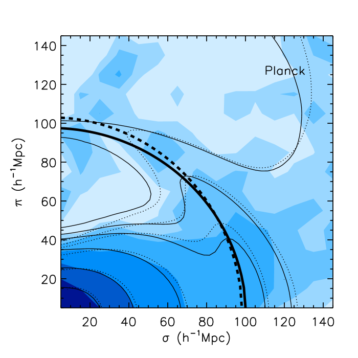
Figure 2: The measured, best fit, and LCDM-predicted versions of $\xi(\sigma,\pi)$ are plotted, using the Planck early universe prior. The blue filled contours represent the measured $\xi(\sigma,\pi)$, and the black unfilled contours represent the best fit $\xi(\sigma,\pi)$ with two different $\sigma_{\rm cut}$. The left panel uses $\sigma_{\rm cut}=20\,h^{-1}\,{\rm Mpc}$ in the fit, and the right panel uses $\sigma_{\rm cut}=40\,h^{-1}\,{\rm Mpc}$. The quarter rings denote the 2D BAO ring, for the fit (solid) and Planck LCDM prediction (dotted).

To fit the correlation function with as model independent cosmology inputs as possible, we assume that the shape of the power spectra is given by the early universe conditions measured by CMB experiments. We denote this primordial spectrum convolved with the transfer function as $D_{m}(k)$. This then evolves coherently through all scales from the last scattering surface. That is, the growth occurs through a time-varying, scale-independent amplitude growth factor (this assumption breaks down in theories that introduce significant scale dependence, such as some modified gravity theories). Propagating this through to cosmological parameters requires assumptions on the cosmological model, e.g. the nature of dark energy. To remain substantially model independent we use the growth rate itself as our variable.

The power spectra are then given by

$$P_{bb}(k,a) = D_{m}(k)G_{b}^{2}(a),$$

$$P_{\Theta\Theta}(k,a) = D_{m}(k)G_{\Theta}^{2}(a)\,,$$ (13)

where $G_{b}$ and $G_{\Theta}$ denote the growth functions of density and peculiar velocity. We define here $G_{b}=b\,G_{\delta_{m}}$ where $b$ is the standard linear bias parameter between galaxy tracers and the underlying dark matter density. The expression of $D_{m}(k)$ is available in Song:2010kq , and assumed to be given precisely by CMB experiments, such as WMAP9 and Planck experiments. We refer to this as an early universe prior. We incorporate the uncertainty from the CMB anisotropy data in the amplitude determination of the initial spectra, $A_{S}^{2}$, into the growth function $G_{X}$, i.e. $G_{X}=G^{*}_{X}A_{S}/A_{S}^{*}$ where $G^{*}_{X}$ is the intrinsic growth function.

The clustering correlation function $\xi(\sigma,\pi)$ is measured in comoving distances, while galaxy locations use angular coordinates and redshift in galaxy redshift surveys. A fiducial cosmology is required for conversion into comoving space. We use the best fit LCDM universe to WMAP9 or Planck. The observed anisotropy correlation function using this model is transformed into true comoving coordinates using the transverse and radial distances, involving $D_{A}$ and $H^{-1}$, respectively. The approximate fiducial maps are created by rescaling the transverse and radial distances, using

$$\sigma^{\rm fid} = \frac{D_{A}^{\rm fid}}{D_{A}^{\rm true}}\ \sigma^{\rm true}$$

$$\pi^{\rm fid} = \frac{H^{-1\,\rm fid}}{H^{-1\,\rm true}}\ \pi^{\rm true}\ ,$$ (14)

where “fid” and “true” denote the fiducial and true distances. Thus the theoretical $\xi$ with potentially true $D_{A}$ and $H^{-1}$ is fitted to the observed $\xi^{\rm fid}$ using the rescaling in the above equations.

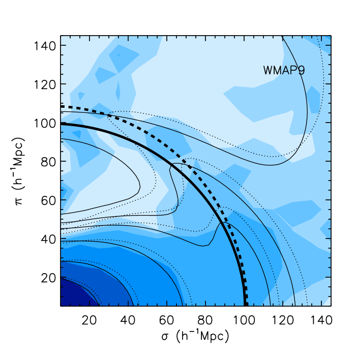
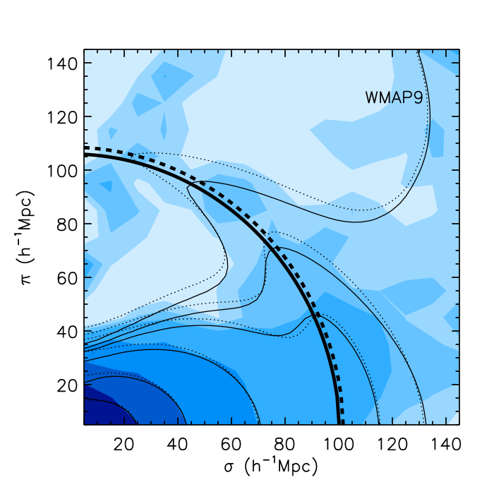
Figure 3: As Fig. 2, but using WMAP9 instead of Planck.

Given the early universe prior on the power spectrum shape, both distances and growth functions are measured simultaneously to high precision Song:2012gh . This holds even without assuming the FRW integral relation between $H^{-1}$ and $D_{A}$. Thus we do not have to assume any particular cosmological model or restrict to zero curvature or LCDM.

Finally, we introduce a parameter representing non–linear contamination to the power spectra of the density and velocity fields. Even on linear scales the damping effect on the power spectrum amplitude caused by random galaxy motions still remains. This is described by the Gaussian model for the FoG effect in Eq. 1, with $\sigma_{p}$ a free parameter giving the velocity dispersion. However, the non–perturbative damping effects are not fully understood, and the Gaussian model may be insuficient on non–linear scales. We therefore do not use the measured $\xi(\sigma,\pi)$ for bins in which this breakdown is likely. Two cut–off’s are used: 1) $s_{\rm cut}$ represents the scales on which non–linear description of $\Delta P_{XY}$ is uncertain, and 2) $\sigma_{\rm cut}$ represents the scales on which Gaussian FoG functional form may not be appropriate. These are set to be $s_{\rm cut}=50\,h^{-1}\,{\rm Mpc}$ and $\sigma_{\rm cut}=40\,h^{-1}\,{\rm Mpc}$ (although we also consider $\sigma_{\rm cut}=20\,h^{-1}\,{\rm Mpc}$). This strategy was tested and proved valid using simulations in our previous work. We follow the same method as presented in Song, Okumura and Taruya (2013) Song:2013ejh .

In summary, we have $G_{b}$ and $G_{\Theta}$ to describe growth functions, $D_{A}$ and $H^{-1}$ to fit distance measures, and $\sigma_{p}$ to model the FoG effect. The form of the FoG is taken to be Gaussian and the shape of the linear spectra is assumed to be given as an early universe prior by CMB experiments.

IV.2 Cut–off scales and 2D BAO ring

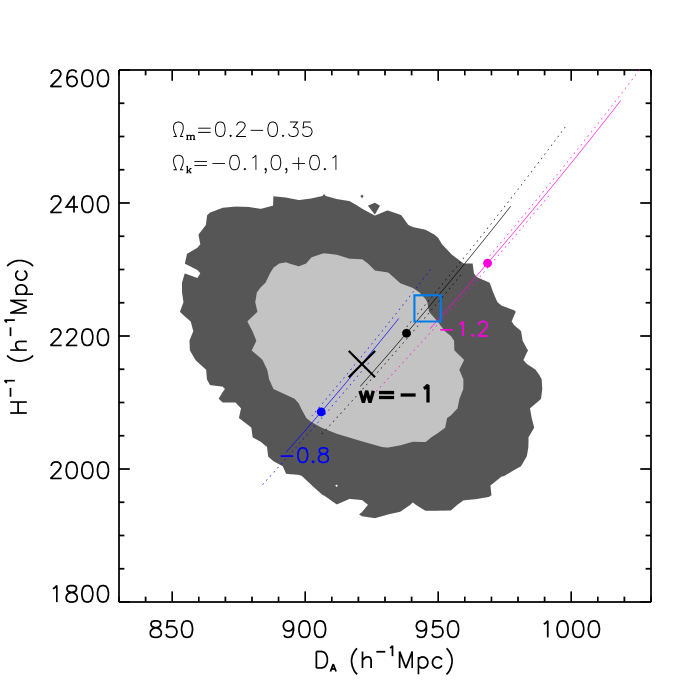
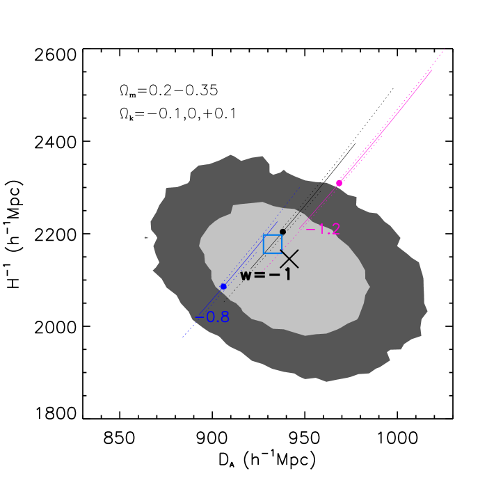
Figure 4: The 68% and 95% confidence contours from the galaxy clustering data are plotted in the $D_{A}-H^{-1}$ plane, with the best fit denoted by the large X. The values predicted from the CMB within LCDM cosmology are shown by the blue square. The left panel uses the WMAP9 early universe prior on the power spectrum shape, while the right panel uses the Planck prior. Overlaid are theory curves giving the relation between the two cosmological quantities within certain cosmologies; note that all standard cosmologies lie in a restricted band. In addition to LCDM (black solid), we show wCDM with $w=-0.8$ (blue) or $w=-1.2$ (magenta), and their generalizations to include spatial curvature (dotted). Each curve covers the range of $\Omega_{m}=0.2$ at their upper ends to $\Omega_{m}=0.35$ at their lower ends, with large dots showing the $\Omega_{m}=0.3$ case.

First, we investigate the appropriate cut–off scales. The $s_{\rm cut}$ is introduced due to the uncertainty of the resummed perturbation theory RegPT at smaller scales. It is conservatively set to be $s_{\rm cut}=50\,h^{-1}\,{\rm Mpc}$ which allows the perfect cross–correlation between density and velocity fields. In addition $\sigma_{\rm cut}$ is used because the improved $\xi(\sigma,\pi)$ in Eq. 2 is not applicable at bins in which the higher order terms of non–perturbative effect are dominant along the line of sight. It was set to be $\sigma_{\rm cut}=20\,h^{-1}\,{\rm Mpc}$ in Song:2013ejh , and reproduced the true values successfully. But we find that it may be too ambitious for the actual DR9 CMASS catalogue.

When the broadband shape of spectra and the distance measures are known, the 2D BAO ring is invariant to the changes of the coherent galaxy bias and coherent motion growth function. When $G_{b}$ increases/decreases, the BAO tip points coherently move counter–clockwise/clockwise. When $G_{\Theta}$ increases/decreases, the BAO tip points move toward/away from the pivot point (equal radial and transverse separation). If the correct distance model is known, the tip points of BAO peaks form an invariant ring regardless of galaxy bias and coherent motion. The ratio between the observed transverse and radial distances varies with the assumed cosmology and, if the shape of an object is a priori known, can provide a measure of $HD_{A}$ (AP test).

The outer measured $\xi(\sigma,\pi)$ contours are too vague to reveal detailed BAO peak structure, but those peak points can define the measured 2D BAO ring. Figure 2 shows the 2D correlation function contours, and the best fit 2D BAO rings. The left and right panels use $\sigma_{\rm cut}=20\,h^{-1}\,{\rm Mpc}$ and $40\,h^{-1}\,{\rm Mpc}$, respectively. If the correlation function model is accurate down to $\sigma_{\rm cut}=20\,h^{-1}\,{\rm Mpc}$ then the two rings should be consistent. However, the 2D BAO ring using $\sigma_{\rm cut}=20\,h^{-1}\,{\rm Mpc}$ not only disagrees with that using $\sigma_{\rm cut}=40\,h^{-1}\,{\rm Mpc}$ but also from the measured circle.

Basically the small, nonlinear scales where the model is imperfect are distorting the results at all scales. This can be seen by looking at several inner contours at small scales, those corresponding to $\xi=(0.2,0.06,0.016,0.005)$. In the left panel the solid curves attempt to fit tightly the small scale contours very close to the line of sight, at the price of a poor fit to the large scale, linear contours. By contrast, in the right panel with $\sigma_{\rm cut}=40\,h^{-1}\,{\rm Mpc}$ the residual non–perturbative effects are observed clearly in the inner contours, but the linear contours are better behaved. This problem with an overambitious use of small scales is seen as well in Fig. 3 using the WMAP9 early universe prior instead.

Therefore we use more conservative bound at $\sigma_{\rm cut}=40\,h^{-1}\,{\rm Mpc}$. We tested our final results using different $\sigma_{\rm cut}$ at 20, 30, 40, and 50 $\,h^{-1}\,{\rm Mpc}$ and found they converged for $\sigma_{\rm cut}\geq 40\,h^{-1}\,{\rm Mpc}$. The effect on cosmology of using a cut allowing more of the non–linear regime is discussed in Sec. V.

The dashed contours in Fig. 2 represent the $\xi(\sigma,\pi)$ of the Planck LCDM concordance model. They are derived using the fiducial $(D_{A},H^{-1},G_{\Theta})$, and best fit $(G_{b},\sigma_{p})$. The right panel of Fig. 2 shows strong agreement between the derived best fit model and the theoretical Planck LCDM concordance model.

For Fig. 3 using the WMAP9 early universe prior, while the estimated 2D BAO ring agrees approximately with the measured 2D BAO ring, peak points along the ring do not well match to each other. The dashed contours here represent $\xi(\sigma,\pi)$ of the WMAP9 LCDM concordance model. Unlike the Planck case, the measured peak points shift toward the pivot point for the outer contour, less so for the inner contours. As discussed above, this is a signature of an increased velocity growth function; we expect the measured $G_{\Theta}$ to be higher than fiducial in this case.

IV.3 The measured distances and growth functions

We present the results for the measured distances and growth functions in Table 1. Our baseline value of $\sigma_{\rm cut}=40\,h^{-1}\,{\rm Mpc}$ is used throughout this section.

Parameters	Fiducial values	Measurements
	With WMAP9 prior
$D_{A}\,(\,h^{-1}\,{\rm Mpc})$	$946.0$	$916.2^{+27.2}_{-25.4}$
$H^{-1}\,(\,h^{-1}\,{\rm Mpc})$	$2241.5$	$2163.1^{+102.0}_{-85.8}$
$G_{b}$	$-$	$1.07^{+0.07}_{-0.09}$
$G_{\Theta}$	$0.44$	$0.51^{+0.09}_{-0.08}$
$\sigma_{p}\,(\,h^{-1}\,{\rm Mpc})$	$-$	$1.0^{+4.6}$
Parameters	Fiducial values	Measurements
	With Planck prior
$D_{A}\,(\,h^{-1}\,{\rm Mpc})$	$932.6$	$939.7^{+26.7}_{-32.6}$
$H^{-1}\,(\,h^{-1}\,{\rm Mpc})$	$2177.5$	$2120.5^{+82.3}_{-100.6}$
$G_{b}$	$-$	$1.11^{+0.07}_{-0.10}$
$G_{\Theta}$	$0.46$	$0.47^{+0.10}_{-0.07}$
$\sigma_{p}\,(\,h^{-1}\,{\rm Mpc})$	$-$	$1.2^{+4.0}$

Table 1: We summarize the values predicted by the CMB data and the values measured from the BOSS data of the distance quantities $D_{A}$ and $H^{-1}$ and the growth quantities $G_{b}$ and $G_{\Theta}$, as well as the velocity damping scale $\sigma_{p}$, with 68% confidence level errors. (The CMB data does not predict values of the astrophysical parameters $G_{b}$ and $\sigma_{p}$.)

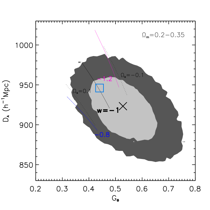
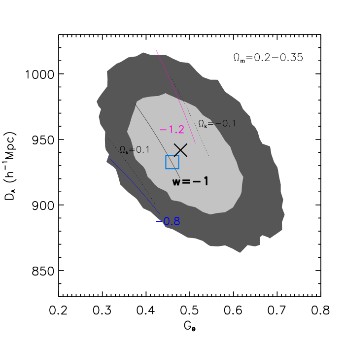
Figure 5: As Fig. 4 but for the $G_{\theta}-D_{A}$ plane. Here the allowed cosmology band is wider (we do not plot the owCDM models).

The angular diameter distance $D_{A}$, related to transverse separations, is measured to be consistent with the LCDM predictions. Most uncertainties of anisotropic distortions are relevant to the radial direction, and it is expected that $D_{A}$ is not biased much. With the Planck early universe prior, $D_{A}$ is measured to be $939.7^{+26.7}_{-32.6}\,h^{-1}\,{\rm Mpc}$, in excellent agreement with the Planck LCDM best fit prediction. Using the WMAP9 early universe prior, the measured $D_{A}$ is $1-\sigma$ from the WMAP9 LCDM prediction.

The line of sight distance quantity $H^{-1}$, related to radial separations, is also measured to be consistent with LCDM predictions. For either the Planck or WMAP9 early universe priors the agreement is within $1-\sigma$. Greater tension is seen if one uses $\sigma_{\rm cut}=20\,h^{-1}\,{\rm Mpc}$, which lowers the measured $H^{-1}$.

As mentioned earlier, the growth functions influence the location of peaks along the rings of power (see Song:2013ejh for illustrations). For the Planck early universe prior, the best fit peak structure is nearly identical to that predicted by the Planck LCDM model. The measured coherent growth function has $G_{\Theta}=0.47^{+0.10}_{-0.07}$, while the fiducial value is $0.46$. This measurement can be converted to a value at $z_{\rm eff}=0.57$ of the standard parameter $f\sigma_{8}=0.48$, which is very close to the fiducial model value of 0.47. When the WMAP9 early universe prior is used, the measured $G_{\Theta}$ becomes bigger than LCDM prediction. Like the distance measurements, the measured $G_{\Theta}$ is offset by $\sim 1-\sigma$.

Note that $G_{\Theta}$ has a relatively large error, about $15-20\%$. This is partly caused by floating $\sigma_{p}$ as a free parameter. In the linear regime, when the first order contribution of the Gaussian FoG function dominates, this factor is nearly featureless and becomes significantly degenerate with coherent growth function. Using more non-linear scales (smaller $\sigma_{\rm cut}$) would break this degeneracy, reducing the error contour but introducing bias; we show this explicitly in Sec. V.

The galaxy bias is estimated from the $G_{b}$ measurement. The bias $b$ is measured to be $1.9$ and $1.8$ for Planck and WMAP9 respectively. Those values are consistent with CMASS catalogues Manera:2012sc . The velocity dispersion $\sigma_{p}$ indicates the level of the FoG effect. For both Planck and WMAP9 cases, it is observed to be small, about $\sigma_{p}=1\,h^{-1}\,{\rm Mpc}$, but with significant uncertainty.

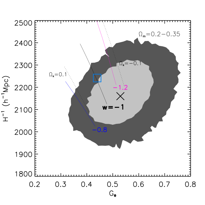
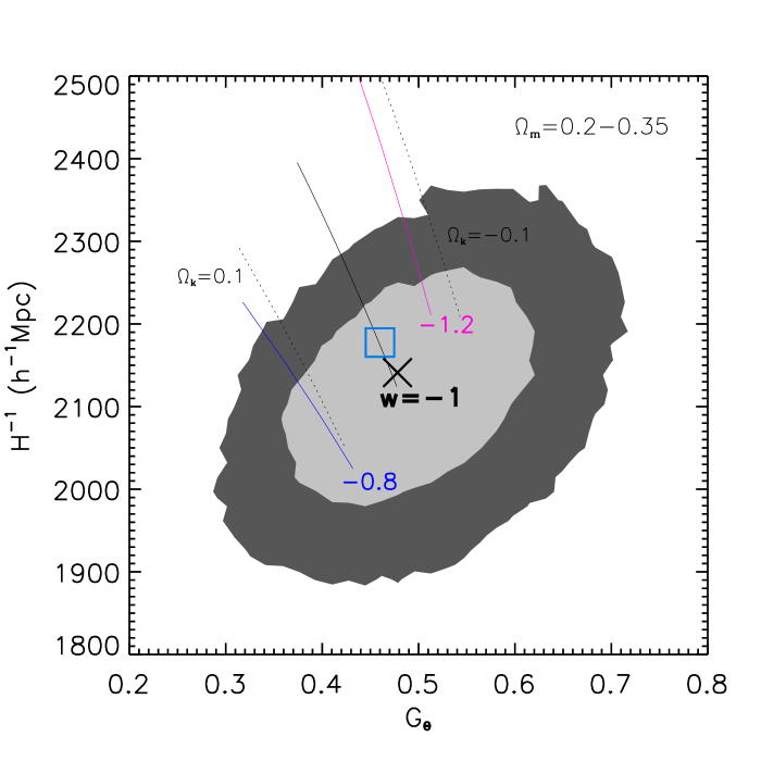
Figure 6: As Fig. 4 but for the $G_{\theta}-H^{-1}$ plane. Here the allowed cosmology band is wider (we do not plot the owCDM models).

V Testing Cosmology

Our analysis approach has been model independent, obtaining constraints on the distances $D_{A}$ and $H^{-1}$ – without even assuming a Friedmann integral relation between them – and on the velocity growth factor $G_{\Theta}$. While we have so far compared the values individually to the best fit LCDM predictions from the CMB, we should also look at the joint probabilities. We can test for consistency with the LCDM model by examining whether the fixed relations between these quantities in LCDM, i.e. the 1D curves in the $D_{A}-H^{-1}$, $D_{A}-G_{\Theta}$, and $H^{-1}-G_{\Theta}$ planes, all intersect the measured confidence contours. Furthermore, we can generalize the test by allowing for spatial curvature or non-$\Lambda$ dark energy. For the growth factor $G_{\Theta}$ this comparison also allows a test of general relativity since within this theory the distance quantities (measuring the cosmic expansion) have a definite relation to the growth quantity $G_{\Theta}$.

Figures 4, 5, 6 show the three planes of pairs of the cosmological quantities and their joint measurement contours, overlaid with the allowed theory curves of LCDM, oLCDM (with spatial curvature), wCDM (dark energy with constant equation of state ratio $w$), and owCDM. Each one is shown for a WMAP9 (left panels) or Planck (right panels) early universe prior.

In the $D_{A}-H^{-1}$ space, the cosmological models all lie within a narrow swath, somewhat separated from the best fit point in the Planck prior case. However, the 68% confidence level contour of the measurements overlaps the LCDM model. In the $D_{A}-G_{\Theta}$ or $H^{-1}-G_{\Theta}$ planes, the standard cosmologies span a wider range of the space. In both planes the measurements are consistent with LCDM at the 68% confidenece level. There is no sign of significant deviation from LCDM in either distances or growth, and hence no sign of deviation from general relativity either.

Note, however, that if we attempt to push the data by using data to smaller, non-linear scales, then we do find deviations. In particular, $G_{\Theta}$ rapidly becomes underestimated, with values of 0.42 for a cutoff at $\sigma_{\rm cut}=30\,h^{-1}\,{\rm Mpc}$ and 0.34 for $\sigma_{\rm cut}=20\,h^{-1}\,{\rm Mpc}$. However increasing $\sigma_{\rm cut}$ above $40\,h^{-1}\,{\rm Mpc}$ does not change the result, indicating the value has converged. Had we included the smaller scales, we would have found that no cosmology (LCDM, oLCDM, wCDM) would have given good fits to the measurement contours. Moreover, we would have apparent evidence for a violation of general relativity. The apparent strong growth suppression in the measured growth rate $G_{\Theta}=d\delta/d\ln a$ would yield an apparent gravitational growth index $\gamma$ Linder (2005) of $\gamma\gtrsim 0.7$, in contrast to the value 0.55 for general relativity.

Figure 7 shows what occurs in the cosmology parameters if data down to $\sigma_{\rm cut}=20\,h^{-1}\,{\rm Mpc}$ is used. The shifting of the best fit values, and the reduction in the uncertainty on $G_{\Theta}$, clearly indicate that substantial information to fit cosmology is coming from small scales, not just the BAO ring scales. Unfortunately, the sensitivity of the results to low $\sigma_{\rm cut}$ (as opposed to the convergence found when $\sigma_{\rm cut}\gtrsim 40\,h^{-1}\,{\rm Mpc}$) indicates that the modeling of the 2D correlation function on these scales is inadequate. Further improvements are necessary before these scales can be used to provide robust results.

In terms of Fourier wavenumber, note that

$$k\approx\frac{2\pi}{\sigma_{\rm cut}}=0.16\,\left(\frac{40\,h^{-1}\,{\rm Mpc}}{\sigma_{\rm cut}}\right)\,h\,{\rm Mpc}^{-1}\ .$$ (15)

In comparisons to simulations the 2D anisotropic clustering model (not simply the 1D real space power spectrum or angle averaged correlation function) performed well down to $40\,h^{-1}\,{\rm Mpc}$ Taruya:2010mx . Another way to spuriously produce a shift outside the swath of standard cosmologies, and hence possibly conclude there is a violation of general relativity, is to misestimate $z_{\rm eff}$. In fact, as we discuss in Appendix A, $z_{\rm eff}$ is itself anisotropic and will differ for different cosmological quantities but not at a level significant with current data.

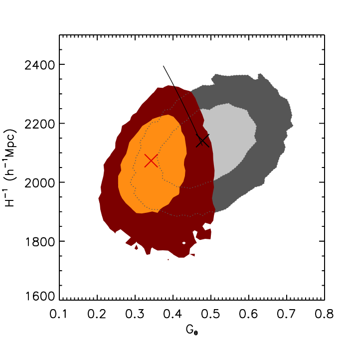
Figure 7: Using small scale information, $\sigma_{\rm cut}=20\,h^{-1}\,{\rm Mpc}$ (in dark orange) rather than our standard $\sigma_{\rm cut}=40\,h^{-1}\,{\rm Mpc}$ (in light grey), shifts the results into a region corresponding to no reasonable cosmology within general relativity. Here we show the $G_{\Theta}-H^{-1}$ plane, with the Planck early universe prior, as an example.

VI Conclusions

We have used the BOSS CMASS DR9 galaxies to perform a cosmology model independent, fully 2D anistropic clustering analysis. Using an early universe prior from CMB experiments, from the clustering correlation function we can extract the angular diameter distance $D_{A}$, Hubble scale $H^{-1}$, and growth rate $G_{\Theta}$ at the effective survey redshift $z_{\rm eff}=0.57$. These are found to be consistent with LCDM, and by comparing expansion of cosmic distances with growth of cosmic structure we also test general relativity, again finding consistency.

Two cautions are relevant to such an analysis, one important already to current data and one entering for future, high precision surveys. Use of small scale measurements of the correlation functions, which can be significantly contaminated by non–linear gravitational physics, is fraught with peril. We find this can distort the cosmological results, moving them wholly outside the range of standard cosmology and give a spurious signature of breakdown of general relativity. Insidiously, the extra data also helps shrink the contours, so the cosmological quantities appear well determined.

We employ the improved redshift distortion model of Taruya:2010mx , but this is still limited in accuracy to scales where higher order terms of the FoG effect are negligible. To prevent bias we cut most of the measured $\xi(\sigma,\pi)$ along the line of sight out from this analysis. This conservative treatment is well defined in the full 2D anisotropy analysis but could be problematic when using a multipole expansion instead. It will be interesting to compare our conservative results to those from a multipole analysis.

Another aspect is that we find that the results from the real, observed, data are more contaminated with the small scale velocity and non-linear effects than those from the mock catalogues. In the simulations, $\sigma_{\rm cut}=20\,h^{-1}\,{\rm Mpc}$ is acceptable to measure observables using the improved perturbation theory model. However, in the real dataset, the cut–off scale must be extended to $\sigma_{\rm cut}=40\,h\,{\rm Mpc}^{-1}$ to obtain convergent results (insensitive to the exact choice of $\sigma_{\rm cut}$). This can also be seen by comparing the 2D BAO ring with the measured BAO peak structure.

The second caution comes from the interpretation dependence of the effective redshift $z_{\rm eff}$. Since it involves the galaxy power spectrum (or correlation function) it is intrinsically anisotropic and will take on different values depending on what quantity is being measured. That is, one formally has $D_{A}(z_{\rm eff}^{D})$, $H^{-1}(z_{\rm eff}^{H})$, etc. We estimate the magnitude of this effect and show that it could become relevant for next generation redshift surveys such as DESI or Euclid.

Appendix A Effective redshift variation

The transverse and radial distances extracted from the galaxy data do not in fact have the same $z_{\rm eff}$, as the optimal weighting depends on the strength of clustering Feldman et al. (1994), enhanced along the line of sight by redshift space distortions [e.g. the usual Kaiser factor $(b+f\mu^{2})^{2}$]. This is most familiar perhaps in the power spectrum, where the weighting $1/[1+n(z)\,P(k,\mu,z)]$ shows that the higher power along the line of sight further deweights lower redshift galaxies where clustering has grown.

This is a small effect, negligible for previous redshift surveys, but will become increasingly important for larger, more precise surveys. Figure 8 calculates $z_{\rm eff}$ as a function of $k$ and $\mu$, using the power spectrum computed from mock simulations relevant to BOSS Okumura et al. (2012). Since most of the information for determining $H^{-1}$ comes from radial modes $\mu\approx 1$ and for determining $D_{A}$ comes from transverse modes $\mu\approx 0$, we see that the fit quantities are really $D_{A}(z_{\rm eff}^{D})$ and $H^{-1}(z_{\rm eff}^{H})$ where $z_{\rm eff}^{H}-z_{\rm eff}^{D}\approx 0.004$. This in turn would affect cosmological parameter estimation.

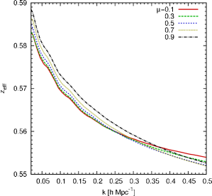
Figure 8: The effective redshift $z_{\rm eff}$ of the galaxy sample depends on the clustering power and hence varies with wavenumber $k$ and redshift distortion angle $\mu$. Observations with most probative power near the $k\approx 0.1\,h\,{\rm Mpc}^{-1}$ have $z_{\rm eff}\approx 0.57$ for this data, but radial modes and transverse modes differ by $\Delta z_{\rm eff}\approx 0.004$, potentially important for future surveys.

Around $z_{\rm eff}\approx 0.57$, the Hubble parameter scales in LCDM as $H(z)\propto 1+z$ so that $dz/(1+z)\approx-dH^{-1}/H^{-1}$. Note that a survey that should use $z_{\rm eff}=0.58$ rather than 0.57, say, due to the anisotropy of $z_{\rm eff}$, would bias $H^{-1}$ by $-0.7\%$. This could be relevant for next generation surveys. Since $D_{A}$ is extracted mostly from the transverse modes where the observed clustering is equal to the real space clustering, no shift should be needed in the conventional $z_{\rm eff}$ estimation. (For completeness we note that if $z_{\rm eff}=0.58$ rather than 0.57 then $D_{A}$ is biased high by 0.8%.) For $G_{\Theta}$ the 2D anisotropy dependence is more complicated (see Fig. 4b of Song:2013ejh ). However, $G_{\theta}$ is near its maximum at $z=0.5$, so a change from $z_{\rm eff}=0.57$ has a very small effect on it; in fact for $z_{\rm eff}=0.58$ the bias is only $-0.0003$ or $-0.06\%$. Thus for current data precision the effect of different $z_{\rm eff}$ for different cosmological parameters is negligible. Next generation galaxy redshift surveys such as DESI or Euclid, however, should adapt $z_{\rm eff}$ to the specific parameter being constrained.

References

- (1) N. Kaiser, Mon. Not. Roy. Astron. Soc. 227, 1 (1987).
- Hamilton (1998) A. J. S., Hamilton 1998, ASSL, 231, 185
- (3) E. V. Linder, Astropart. Phys. 29, 336 (2008)
- (4) S. F. Daniel and E. V. Linder, Phys. Rev. D 82, 103523 (2010)
- (5) A. Shafieloo, A. G. Kim and E. V. Linder, Phys. Rev. D 87, 023520 (2013)
- (6) L. Guzzo, M. Pierleoni, B. Meneux, E. Branchini, O. L. Fevre, C. Marinoni, B. Garilli and J. Blaizot et al., Nature 451, 541 (2008)
- (7) Y. -S. Song and W. J. Percival, JCAP 0910, 004 (2009)
- (8) Y. -S. Song, L. Hollenstein, G. Caldera-Cabral and K. Koyama, JCAP 1004, 018 (2010)
- (9) Y. -S. Song, G. -B. Zhao, D. Bacon, K. Koyama, R. C. Nichol and L. Pogosian, Phys. Rev. D 84, 083523 (2011)
- (10) B. A. Reid, L. Samushia, M. White, W. J. Percival, M. Manera, N. Padmanabhan, A. J. Ross and A. G. Sanchez et al., arXiv:1203.6641 [astro-ph.CO].
- (11) B. Jain and P. Zhang, Phys. Rev. D 78, 063503 (2008)
- (12) P. Zhang, M. Liguori, R. Bean and S. Dodelson, Phys. Rev. Lett. 99, 141302 (2007)
- (13) Y. Wang, JCAP 0805, 021 (2008)
- (14) J. Yoo and U. Seljak, Phys. Rev. D 86, 083504 (2012)
- (15) R. Reyes, R. Mandelbaum, U. Seljak, T. Baldauf, J. E. Gunn, L. Lombriser and R. E. Smith, Nature 464, 256 (2010)
- (16) C. Alcock and B. Paczynski, Nature 281, 358 (1979).
- (17) N. Padmanabhan and M. J. White, 1, Phys. Rev. D 77, 123540 (2008)
- (18) E. Gaztanaga, A. Cabre and L. Hui, Mon. Not. Roy. Astron. Soc. 399, 1663 (2009)
- Ballinger et al. (1996) W. E., Ballinger, J. A., Peacock, A. F., Heavens 1996, MNRAS, 282, 877
- Matsubara & Suto (1996) T., Matsubara, & Y. Suto 1996, ApJL, 470, 1
- Blake & Glazebrook (2003) C., Blake & K., Glazebrook (2003) Astrophys. J. , 594, 665
- Eisenstein et al. (2005) D. J., Eisenstein, et al. (2005) Astrophys. J. , 633, 560
- (23) Y. -S. Song, T. Okumura and A. Taruya, arXiv:1309.1162 [astro-ph.CO].
- (24) W. Hu and Z. Haiman, Phys. Rev. D 68, 063004 (2003)
- (25) C. P. Ahn et al. [SDSS Collaboration], Astrophys. J. Suppl. 203, 21 (2012)
- (26) L. Anderson, E. Aubourg, S. Bailey, F. Beutler, A. S. Bolton, J. Brinkmann, J. R. Brownstein and C. -H. Chuang et al., arXiv:1303.4666 [astro-ph.CO].
- Busca et al. (2013) N. G. Busca, T. Delubac, J. Rich, et al. 2013, AA, 552, A96
- (28) A. G. Sanchez, E. A. Kazin, F. Beutler, C. -H. Chuang, A. J. Cuesta, D. J. Eisenstein, M. Manera and F. Montesano et al., arXiv:1303.4396 [astro-ph.CO].
- (29) E. A. Kazin, A. G. Sanchez, A. J. Cuesta, F. Beutler, C. -H. Chuang, D. J. Eisenstein, M. Manera and N. Padmanabhan et al., arXiv:1303.4391 [astro-ph.CO].
- Samushia et al. (2013) L. Samushia, B. A. Reid, M. White, et al. 2013, MNRAS, 429, 1514
- Ross et al. (2013) A. J. Ross, W. J. Percival, A. Carnero, et al. 2013, MNRAS, 428, 1116
- (32) R. Scoccimarro, Phys. Rev. D 70, 083007 (2004)
- Okumura et al. (2008) T., Okumura, T., Matsubara, D. J., Eisenstein, I., Kayo, C., Hikage, A. S., Szalay, & D. P., Schineider (2008) Astrophys. J. , 676, 889
- Matsubara (2004) T., Matsubara (2004) Astrophys. J. , 615, 573
- (35) Y. -S. Song, C. G. Sabiu, I. Kayo and R. C. Nichol, JCAP 1105, 020 (2011)
- (36) A. Taruya, T. Nishimichi and S. Saito, Phys. Rev. D 82, 063522 (2010)
- (37) A. Taruya and T. Hiramatsu, arXiv:0708.1367 [astro-ph].
- (38) A. Taruya, F. Bernardeau, T. Nishimichi and S. Codis, Phys. Rev. D 86, 103528 (2012)
- (39) Y. -S. Song, T. Nishimichi, A. Taruya and I. Kayo, Phys. Rev. D 87, 123510 (2013)
- York et al. (2000) D. G. York, J. Adelman, J. E. Jr. Anderson, et al. 2000, AJL, 120, 1579
- Maraston et al. (2009) C. Maraston, G. Strömbäck, D. Thomas, D. A. Wake, & R. C. Nichol, 2009, MNRAS, 394, L107
- Nuza et al. (2013) S. E. Nuza, A. G. Sánchez, F. Prada, et al. 2013, MNRAS, 432, 743
- (43) The data and random catalogues are available online at http://data.sdss3.org/sas/dr9/boss/
- Cannon et al. (2006) R. Cannon, M. Drinkwater, A. Edge, et al. 2006, MNRAS, 372, 425
- Anderson et al. (2012) L. Anderson, E. Aubourg, S. Bailey, et al. 2012, MNRAS, 427, 3435
- Ross et al. (2012) A. J. Ross, W. J. Percival, A. G. Sánchez, et al. 2012, MNRAS, 424, 564
- Feldman et al. (1994) H. A. Feldman, N. Kaiser, & J. A. Peacock, 1994, Astrophys. J. , 426, 23
- Landy & Szalay (1993) S. D. Landy, & A. S. Szalay, 1993, Astrophys. J. , 412, 64
- (49) M. Manera, R. Scoccimarro, W. J. Percival, L. Samushia, C. K. McBride, A. Ross, R. Sheth and M. White et al., Mon. Not. Roy. Astron. Soc. 428, no. 2, 1036 (2012)
- Song et al. (2010) Y.-S. Song, C. G. Sabiu, R. C. Nichol, & C. J. Miller, 2010, J. Cosmology Astropart. Phys., 1, 25
- Hartlap et al. (2007) J. Hartlap, P. Simon, & P. Schneider 2007, AA, 464, 399
- (52) Y. -S. Song, Phys. Rev. D 87, 023005 (2013)
- Linder (2005) E. V. Linder, 2005, Phys. Rev. D, 72, 043529
- Okumura et al. (2012) T., Okumura, U., Seljak, & V., Desjacques (2012) J. Cosmology Astropart. Phys., 11, 014 [arXiv:1206.4070]