A High Angular Resolution Survey of Massive Stars in Cygnus OB2: Results from the Hubble Space Telescope Fine Guidance Sensors

S. M. Caballero-Nieves¹¹affiliation: Current Address: Department of Physics and Astronomy University of Sheffield, Hounsfield Road, Sheffield S3 7RH, UK; s.caballero@shef.ac.uk ²²affiliation: Center for High Angular Resolution Astronomy, Department of Physics and Astronomy, Georgia State University, P. O. Box 4106, Atlanta, GA 30302-4106, USA; gies@chara.gsu.edu, jao@chara.gsu.edu , E. P. Nelan³³affiliation: Space Telescope Science Institute, 3700 San Martin Drive, Baltimore, MD 21218, USA; nelan@stsci.edu, walborn@stsci.edu , D. R. Gies²²affiliation: Center for High Angular Resolution Astronomy, Department of Physics and Astronomy, Georgia State University, P. O. Box 4106, Atlanta, GA 30302-4106, USA; gies@chara.gsu.edu, jao@chara.gsu.edu , D. J. Wallace⁴⁴affiliation: Department of Natural Sciences, University of South Carolina Beaufort, 1 University Boulevard, Bluffton, SC 29909, USA; debra.j.wallace@nasa.gov , K. DeGioia-Eastwood⁵⁵affiliation: Department of Physics and Astronomy, Northern Arizona University, P.O. Box 6010, Flagstaff, AZ 86011-6010, USA; kathy.eastwood@nau.edu , A. Herrero⁶⁶affiliation: Instituto de Astrofísica de Canarias, C/ Via Lactea s/n, E-38280 La Laguna, Spain and Departamento de Astrofísica, Universidad de La Laguna, Avda. Astrofísico Francisco Sánchez, 2, E-38205 La Laguna, Spain; ahd@iac.es , W.-C. Jao²²affiliation: Center for High Angular Resolution Astronomy, Department of Physics and Astronomy, Georgia State University, P. O. Box 4106, Atlanta, GA 30302-4106, USA; gies@chara.gsu.edu, jao@chara.gsu.edu , B. D. Mason⁷⁷affiliation: U. S. Naval Observatory, 3450 Massachusetts Avenue, NW, Washington, DC 20392-5420, USA; brian.mason@usno.navy.mil , P. Massey⁸⁸affiliation: Lowell Observatory, 1400 West Mars Hill Road, Flagstaff, AZ 86001, USA; massey@lowell.edu , A. F. J. Moffat⁹⁹affiliation: Département de physique, Université de Montréal, CP 6128, Succ. Centre-Ville, Montréal, QC H3C 3J7, Canada; moffat@astro.umontreal.ca , N. R. Walborn³³affiliation: Space Telescope Science Institute, 3700 San Martin Drive, Baltimore, MD 21218, USA; nelan@stsci.edu, walborn@stsci.edu

Abstract

We present results of a high angular resolution survey of massive OB stars in the Cygnus OB2 association that we conducted with the Fine Guidance Sensor 1R (FGS1r) on the Hubble Space Telescope. FGS1r is able to resolve binary systems with a magnitude difference $\Delta V<4$ down to separations as small as $0\farcs 01$ . The sample includes 58 of the brighter members of Cyg OB2, one of the closest examples of an environment containing a large number of very young and massive stars. We resolved binary companions for 12 targets and confirmed the triple nature of one other target, and we offer evidence of marginally resolved companions for two additional stars. We confirm the binary nature of 11 of these systems from complementary adaptive optics imaging observations. The overall binary frequency in our study is 22% to 26% corresponding to orbital periods ranging from 20 - 20,000 years. When combined with the known short-period spectroscopic binaries, the results supports the hypothesis that the binary fraction among massive stars is $>60$ %. One of the new discoveries is a companion to the hypergiant star MT 304 = Cyg OB2-12, and future measurements of orbital motion should provide mass estimates for this very luminous star.

techniques: high angular resolution — binaries: visual — stars: early-type — stars: massive — open clusters and associations: individual: Cyg OB2

^†^†slugcomment: Draft 09/13/2013

1 Introduction

Massive stars ( $\gtrsim 10M_{\odot}$ ) play a fundamental role in the evolution of the universe, from influencing galactic dynamics and structure to triggering star formation through their spectacularly violent deaths. It has been well established that massive stars have a higher binary frequency than lower mass stars (Mason et al., 2009; Raghavan et al., 2010), and the binary fraction may be as high as 100% for massive stars in clusters and associations (Mason et al., 1998, 2009; Kouwenhoven et al., 2007; Chini et al., 2012). Because most massive stars are born in clusters and associations, their multiplicity properties offer important clues about their formation processes (Zinnecker & Yorke, 2007). However, our knowledge about the numbers and distributions of binary and multiple stars is incomplete because the systems are generally so distant that we cannot detect binaries in the separation realm between spectroscopically detected systems and angularly resolved systems, i.e., those with small angular separations and periods in the range of years to decades (Mason et al., 1998). We need milliarcsecond (mas) resolution to start to fill in this observational period gap (Sana et al., 2008).

The Orion Nebula cluster provides the closest example ( $d=0.41$ kpc; Menten et al. 2007) of an environment with a modest number of massive O-stars (Preibisch et al., 1999; Weigelt et al., 1999; Close et al., 2012). However, to explore a large sample of very massive stars, the next closest environment is the association Cygnus OB2 at a distance of $d=1.40\pm 0.08$ kpc (Rygl et al., 2012). The Cyg OB2 association has approximately $2600\pm 400$ members (Knödlseder, 2000) with about 100 O-stars within the central 1^∘ (Comerón et al., 2002; Wright et al., 2010), making it one of the largest concentrations of OB stars in the Galaxy. It is home to some of the most massive ( $M>100M_{\odot}$ ; Massey & Thompson 1991; Knödlseder 2000; Herrero et al. 2001) and intrinsically brightest stars (MT 304; Massey & Thompson 1991) known in our Galaxy, including two of the rare O3-type stars (MT 417 and MT 457; Walborn et al. 2002; Walborn 1973, respectively). The close binary properties of the Cyg OB2 stars have been studied extensively in the spectroscopic survey of Kiminki & Kobulnicky (2012) (and references therein). A few wider systems have been identified through high angular resolution speckle (Mason et al., 2009) and imaging observations (Maíz Apellániz, 2010).

The Fine Guidance Sensors (FGS) aboard the Hubble Space Telescope (HST) provide us with the means to search for visual binaries among the optically faint, massive stars of Cyg OB2. FGS TRANS mode observations can resolve systems with separations of $0\farcs 01-1\arcsec$ , or 14-1400 AU (or 2800 AU in the case of MT 417 with a $2\farcs 5$ scan length) and differential magnitudes less than about 4 mag (Horch et al., 2006; Nelan et al., 2012). At these separations we are sampling systems where the components would evolve independently of each other but are nevertheless important in understanding massive star formation. Due to the short length of the scans ( $\sim 1\arcsec$ ) the sources we find are highly probable to be true companions. We will discuss the probability of chance alignments in our sample in a future paper (Caballero-Nieves et al., in prep.). Nelan et al. (2004) used the FGS instrument to search for binaries among 23 massive stars in the Carina Nebula region ( $d\approx 2.5$ kpc), and they discovered five new binaries, including a companion of the very massive star HD 93129A at a separation of 53 mas (133 AU). Here we present the results of an FGS survey for visual binaries around 58 stars in Cyg OB2. We compare the results with those from an infrared adaptive optics survey that will be presented in a future paper. In section 2 we describe the sample selection, observations, and the FGS reduction pipeline and process. Section 3 describes how binary stars are detected, and section 4 details the fitting routines used to determine the system parameters (differential magnitude, angular separation, and position angle). The detection limits for our sample are also discussed there. Our results are presented in section 5, and a discussion of the multiplicity of our sample and future work is given in section 6.

2 Sample and Observations

The stars were selected from among the brightest, most massive stars in Cyg OB2 as cataloged in Schulte (1958), Massey & Thompson (1991), and Comerón et al. (2002). All the stars in our sample have published spectral classifications and are brighter than $V=14$ mag, well within the detection limits of FGS. The observations were scheduled under HST proposal 10612 (PI: D. Gies), a SNAP program with 70 available targets. SNAP programs are used when needed to fill gaps in HST’s observing schedule which cannot be filled by the GO class programs. Typically 50% of the targets in a SNAP program are actually observed, our program faired better with 58 stars observed, listed in Table 1. The stars are identified according to the numbering scheme used in the optical photometric survey of Massey & Thompson (1991) (e.g., MT 138) and the infrared spectroscopic study of Comerón et al. (2002) (e.g., A 23). Stars not included in those surveys are identified by the number assigned by Schulte (1958) (e.g., SCHULTE 5 = S 5 = Cyg OB2-5) or by the Wolf-Rayet number from van der Hucht (2001) (e.g., WR 145). Table A High Angular Resolution Survey of Massive Stars in Cygnus OB2: Results from the Hubble Space Telescope Fine Guidance Sensors also lists the celestial coordinates from 2MASS (Skrutskie et al., 2006), spectral classification and reference source, $V$ magnitude, $B-V$ color, date of observation, the name of the single star whose observation was used as the calibrator for the binary fitting, and the number of components detected. The stars from Comerón et al. (2002) do not have known $B-V$ colors, but because they are bright infrared sources, they are assumed to be redder than the other stars in the survey. The final column indicates known binary systems detected through our adaptive optics program or through the spectroscopic observations of Kiminki et al. (2012). ‘NIRI’ in the remarks column denotes systems that we resolved in a $K$ -band survey made with the NIRI camera and Altair adaptive optics system on the Gemini North Telescope (Caballero-Nieves, 2012). ‘RV constant’ indicates objects observed by Kobulnicky et al. (2012) that did not show radial velocity variability during the course of their survey. Spectroscopic binaries are denoted by ‘SB1’ and ‘SB2’ for those detected by single-lined or double-lined radial velocity variations, respectively (Kiminki et al., 2012). Eclipsing binaries are denoted by ‘EW/KE’ (W UMa type with ellipsoidal variations and periods $P<1$ d), ‘EA’ (detached systems with flat maxima), and ‘EB’ (semi-detached with ellipsoidal light curves) (Kiminki et al., 2012). At the time of writing, 32 stars out of the 58 observed are known multiple systems; 9 are angularly resolved systems listed in the Washington Double Star catalog (Mason et al., 2001), two of which are also spectroscopic binaries from the 25 systems detected by Kiminki et al. (2012).

All the stars were observed using FGS1r in its high angular resolution TRANSFER mode (TRANS). The FGS is a Koesters prism based, white light, shearing interferometer that is sensitive to the tilt of the incident wave front from a luminous object. The FGS optical train includes a polarizing beam splitter that illuminates two mutually orthogonal Koesters prisms which provides simultaneous sensitivity to the wavefront tilt along the FGS’s $x$ - and $y$ -axes. In TRANSFER mode the the FGS $5\arcsec\times 5\arcsec$ instantaneous field of view (IFOV) is scanned across the object of interest along a 45 degree path in the FGS ( $x$ , $y$ ) coordinate frame, which varies the incoming wavefront tilt along both axes. If the source is a resolved binary, the light from the two stars will be mutually incoherent and the observed interference fringe will differ from that of an unresolved point source (Nelan et al., 2012). We observed each star using 20 scans with a scan length of 1″ composed of 1 milli-arcsecond steps (for MT 417 we employed a $2\farcs 5$ scan length to capture each component of this known wide binary). All observations were made using the F583W filter, which has a central wavelength of 5830 Å and a passband of 3400 Å.

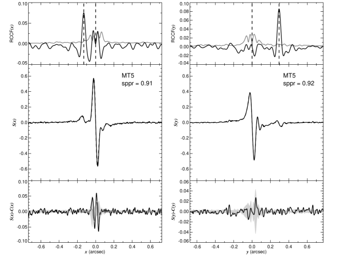
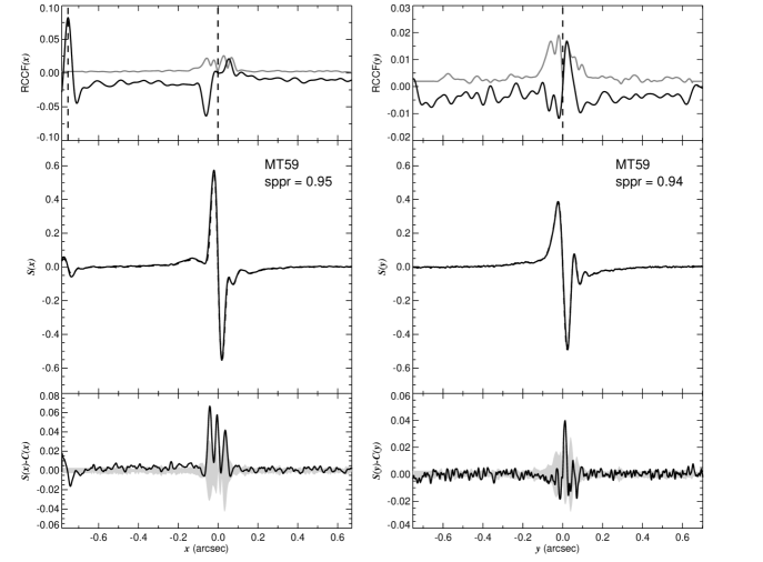
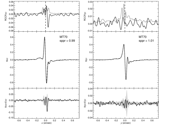
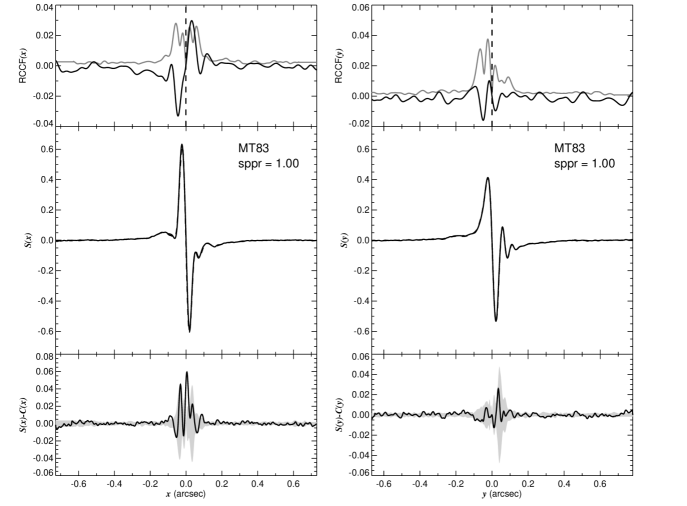
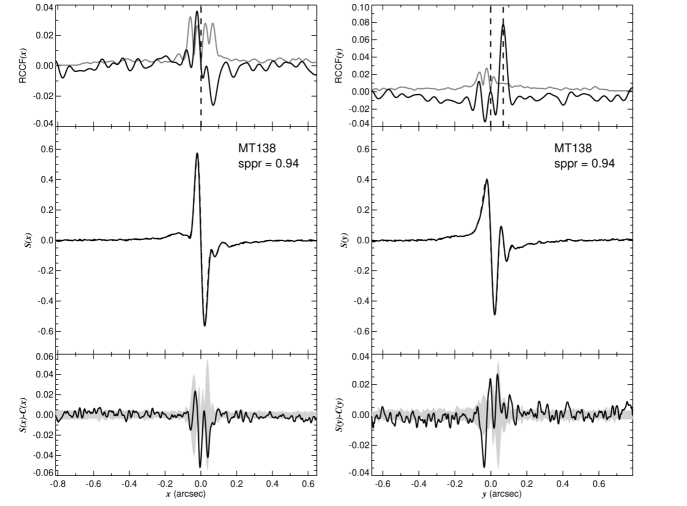
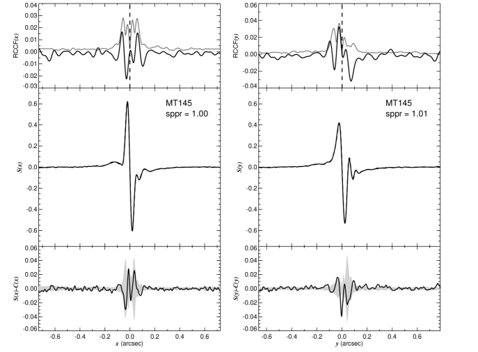
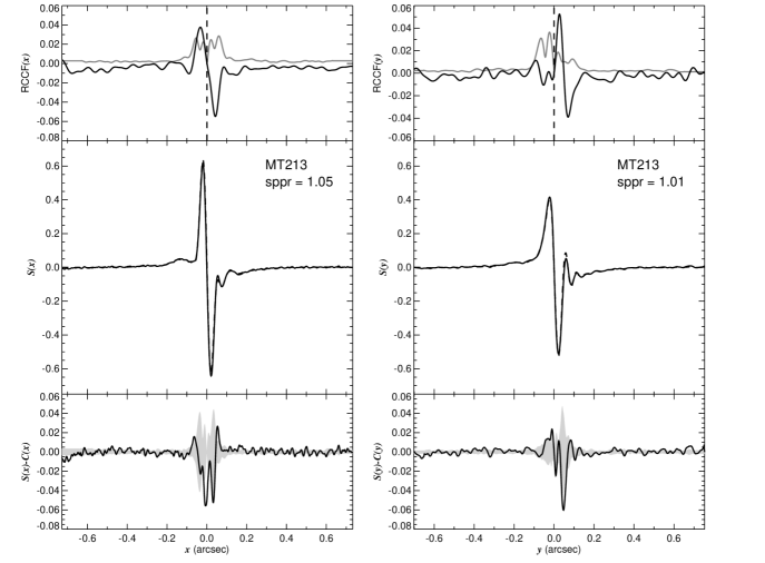
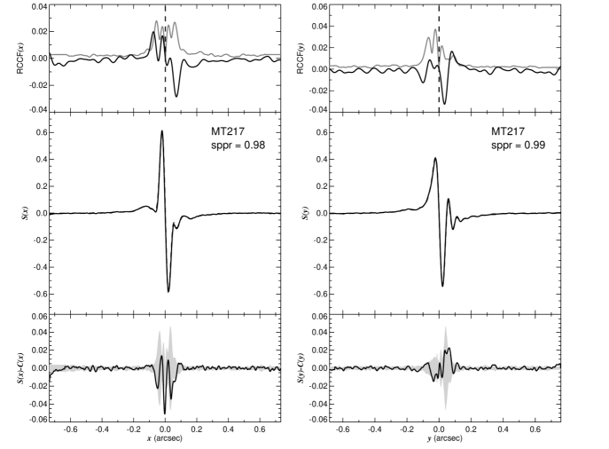
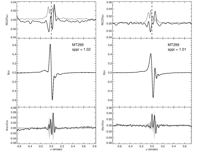
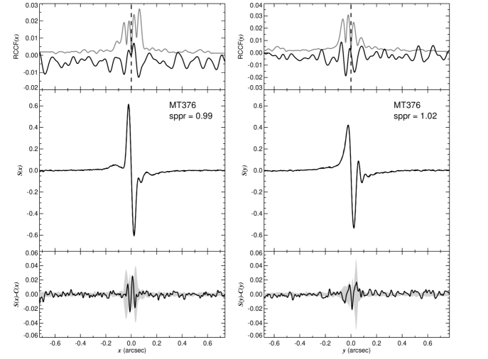
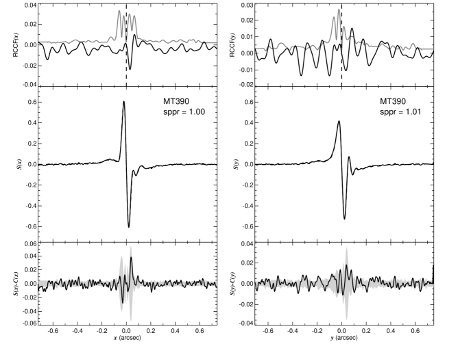
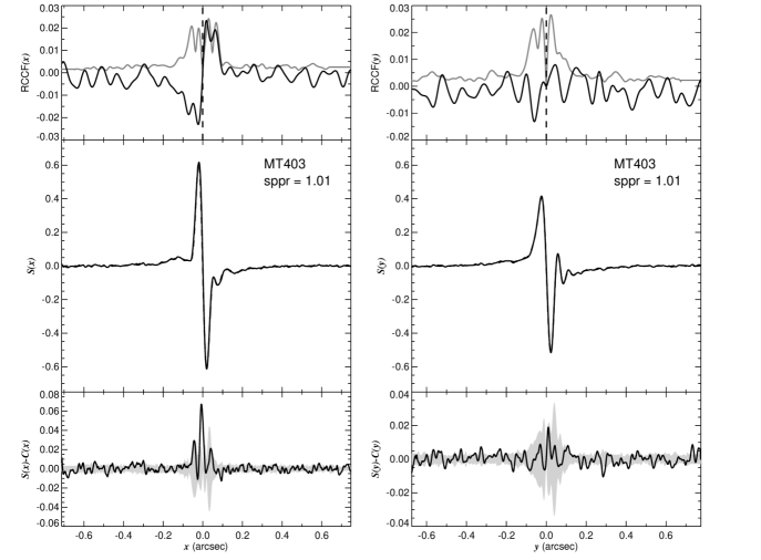
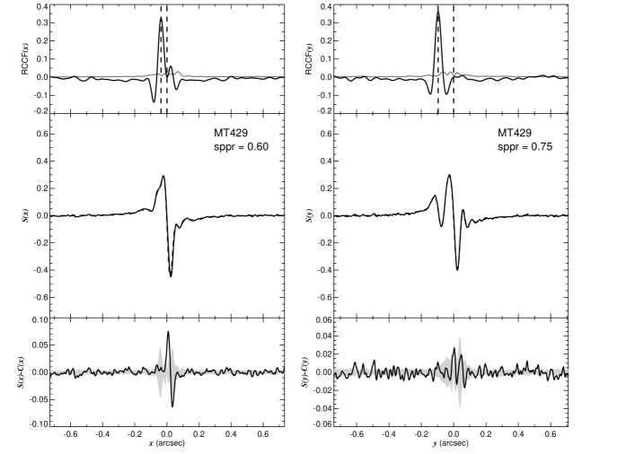
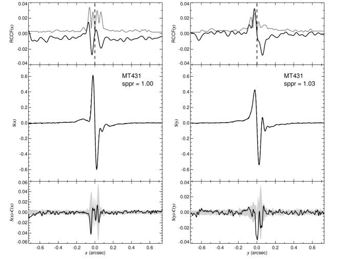
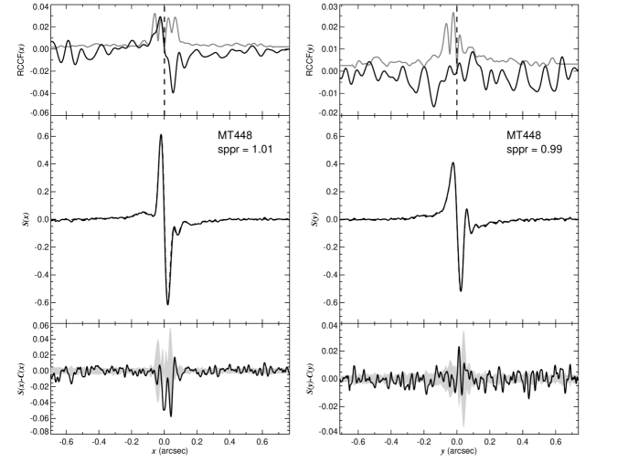
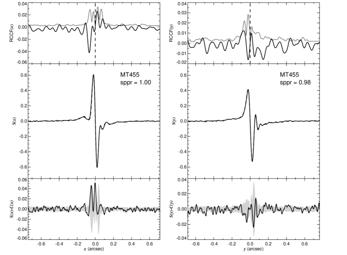
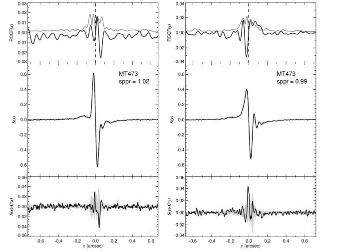
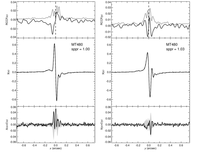
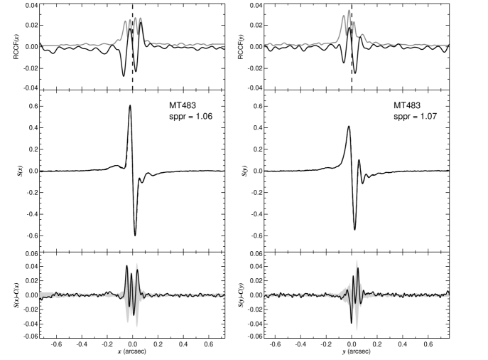
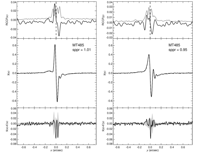
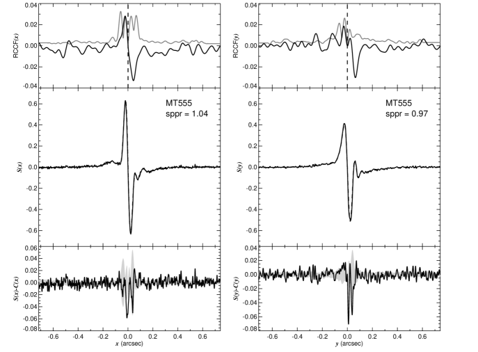
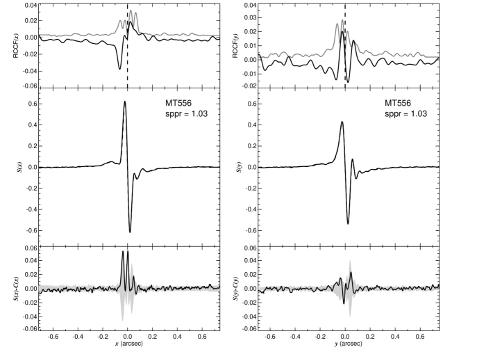
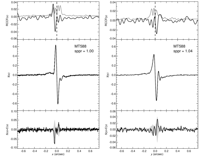
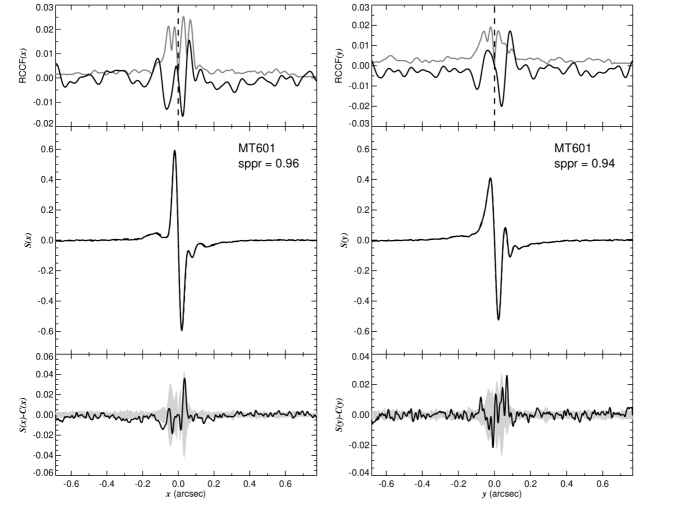
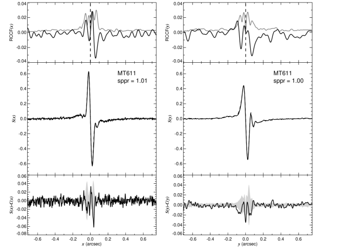
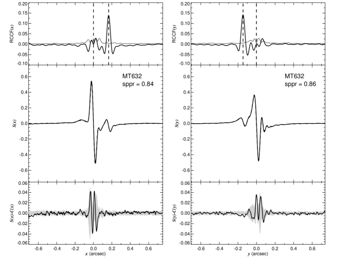
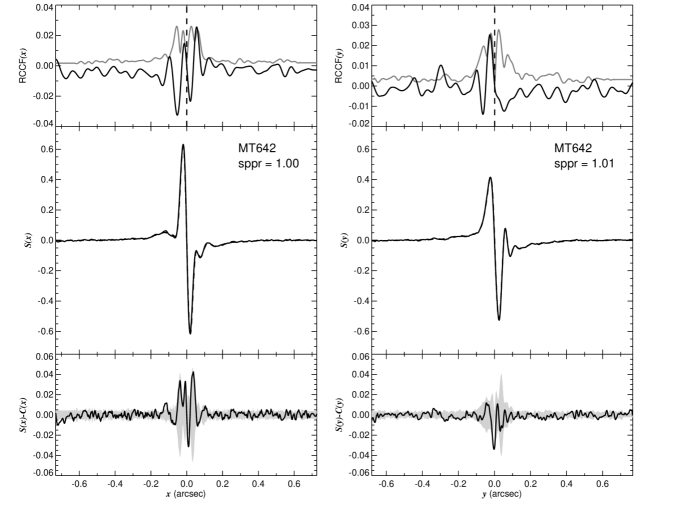
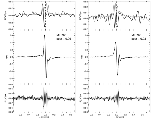
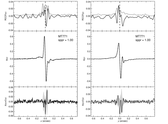
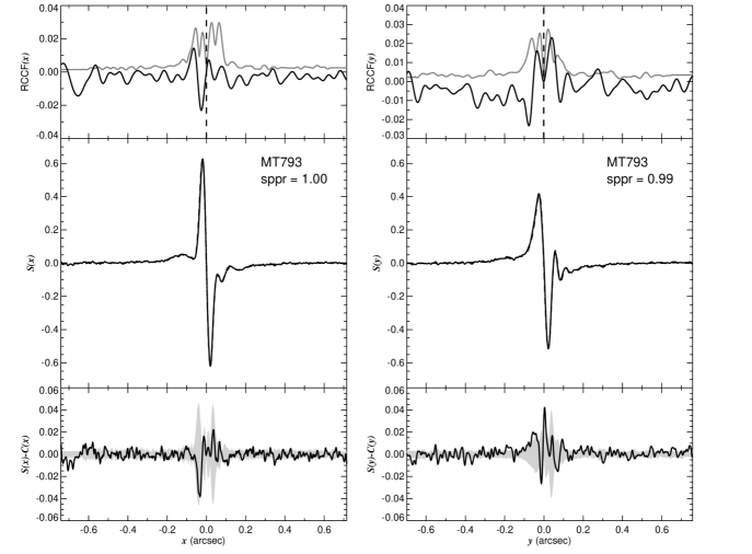
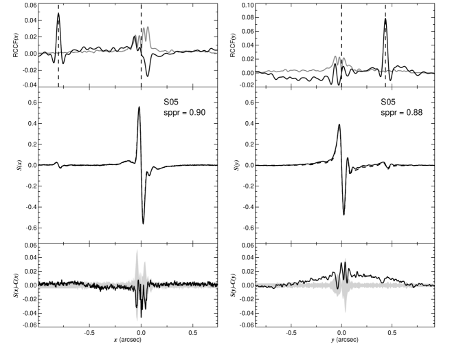
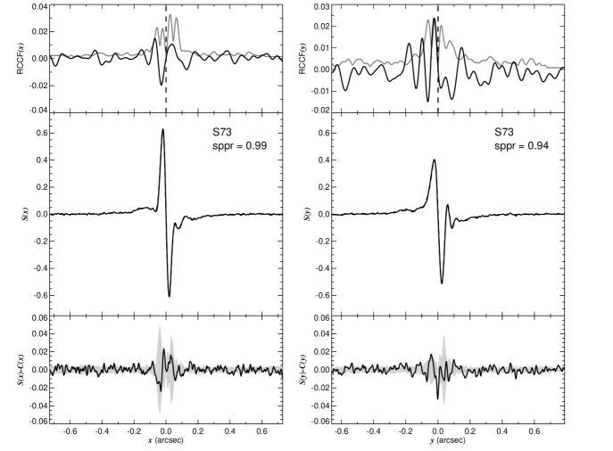
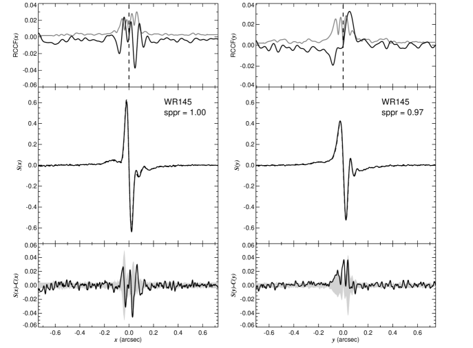
The resultant interference fringes, traditionally referred to as “ $S$ -curves” due to their characteristic shape, are reconstructed from the photon counts reported by the photo-multiplier tubes (PMTs) at each step of the scan using the FGS data reduction pipeline. The reconstructed individual scans are cross correlated to optimize mutual alignment (eliminating spacecraft drift). Once aligned, the scans are co-added and then smoothed using a piecewise spline fit to obtain the optimal signal-to-noise ratio of the final $S$ -curve. Any scan found to be excessively noisy (from high spacecraft jitter) was deleted from the process. We found that it was helpful to remove the low frequency, slowly varying background of the scans because of their increasing departure from zero difference with increasing separation from the central fringe (caused by spatial sensitivity variations of the photomultiplier tubes). This was usually accomplished by subtracting a parabolic fit of the outer fringe pattern, or wings, determined from the mean of many calibrator (single) star scans. However, in a few cases the outer fringe variation was too large to be rectified this way, and a spline fit was made of the fringe variation at representative points along the $S$ -curve. The final $S$ -curves for all of the stars are presented in alphabetical order in Figure Set 1 (available in full in the electronic version of the paper). The $S$ -curves appear in the middle panels for both the $x$ - and $y$ -axes while the upper and lower panels summarize searches for resolved and blended companions, respectively (see section 3).

3 Companion Detection

Binaries display an $S$ -curve that appears as the sum of two offset and rescaled fringe patterns (see section 3.2). A binary detection is made by comparing the $S$ -curve of a target to that of a point-source (single star). We describe below the three detection methods we used to determine binarity. The comparison star, or calibrator, is taken from unresolved sources within our sample that meet three criteria: (1) observed using the same filter, (2) close in $B-V$ color, and (3) close in observation date. The first criterion is met by all the stars in our sample. Criterion 2 is necessary because the appearance of a point source $S$ -curve is color dependent due to refractive optics within the FGS and the wavelength dependent response of the PMTs. For example, the shape of an $S$ -curve is slightly broadened for redder targets (Horch et al., 2006). We chose calibrators whose colors are within $\pm 0.2$ mag from the target $B-V$ , except for a few very red stars (section 4). The appearance of the $S$ -curves can change with time due to the settling of the instruments and adjustments from servicing missions. Our observing program was not affected by any changes made due to a servicing mission, but our large range of observation dates (2005 December to 2008 June) spans a range where the long term changes in FGS1r, while small, are non-negligible. Thus, we chose as the best calibrator the one observed closest in time to the target. The binary systems we are able to resolve have components with nearly equal brightness and hence, their colors should be comparable in most cases. Consequently, we adopted the same calibrator to model both components.

3.1 Visual Inspection

The $S$ -curve or transfer function of a binary consists of the normalized superposition of the individual transfer functions of two point sources. For widely separated systems, the scan will show two shifted transfer functions, whose relative amplitudes are directly related to the magnitude difference (see eq. 3). For closer systems, the $S$ -curve can look obviously different from that of a single star (such as the case of MT 429 shown in Fig. 1.25), because the composite fringe is formed from two overlapping fringes. Thus, a direct comparison of the smoothed, co-aligned, target $S$ -curve with that of a single star provides the first way to identify binaries.

Another indicator of a resolved binary is the relative fringe amplitude, calculated as the value of $sppr$ , or the $S$ -curve peak-to-peak ratio. The ratio of the extrema points of the fringe to that of a single star calibrator fringe can be expressed as

sppr=\frac{S_{\rm obs,max}-S_{\rm obs,min}}{S_{\rm F583W,max}-S_{\rm F583W,min}}

(1)

where, for bright stars ( $V<12$ ), $S_{\rm F583W,max}=0.61$ and $S_{\rm F583W,min}=-0.55$ along the $x$ -axis and $S_{\rm F583W,max}=0.30$ and $S_{\rm F583W,min}=-0.65$ along the $y$ -axis for typical single star observations made with the F583W filter. This parameter is listed in the middle panels of Figure Set 1 using denominator values from the mean of the selected calibrator $S$ -curves. The cases where $sppr\leq 0.9$ indicate that the target is a resolved binary in which destructive interference causes a decline in the overall fringe amplitude. However, if $0.9\leq sppr\leq 1.0$ , as would be the case for a binary with a small angular separation or large magnitude difference of the components, a more thorough analysis is needed. Note that the $x$ - and $y$ - axes have different values; this is due to the effect of the HST spherical aberration and the alignment of the interferometer optical elements relative to the HST optical axis. Also note that the $S_{\rm F853W,max}$ and min values are adjusted for the magnitude of the target since the $S$ -curve is also affected by the PMT dark current, which becomes an increasing larger percentage of the total counts as fainter targets are observed. This effect is negligible for $V<12$ , but is significant for fainter objects. Note, the initial $sppr$ value used as a quick-look tool for a companion was computed from the scans that have not been de-jittered, cross correlated, or smoothed as they are for the more thorough analysis described in the next sections. The $sppr$ values quoted in Figure Set 1 are calculated after this analysis has been performed, but do not differ significantly from the initial $sppr$ value used.

We produced an initial list of stars that appeared single according to the visual inspection and the $sppr$ filter as possible calibrators for the analysis described in the following sections. From there, we narrowed the list through an iterative process of selecting which stars met the following criteria for point sources, and we used those as the calibrators for modeling purposes.

3.2 Marginally Resolved Systems and Detection Limits

Close systems (projected separation $\lesssim 25$ mas), where the two $S$ -curves are not well separated, can slightly reduce the fringe amplitude and widen the fringe shape. If the fringe pattern of a single calibrator star is $S(x)$ , then the observed fringe pattern for more than one star will be

S(x)_{obs}=\sum_{i=1}^{n}f_{i}~{}S(x-x_{i})

(2)

where each of $n$ stars has a flux fraction $f_{i}=\frac{F_{i}}{\sum F_{j}}$ and a relative projected offset position $x_{i}$ . For a binary star with a companion flux ratio $r=\frac{F_{2}}{F_{1}}$ and a projected separation $\Delta x$ , the observed pattern simplifies to

S(x)_{obs}=\frac{1}{1+r}S(x)+\frac{r}{1+r}S(x-\Delta x).

(3)

An analytical representation of the difference between the binary and calibrator $S$ -curves can be estimated by making a second-order expansion for small offset $\epsilon$ ,

S(x+\epsilon)=S(x)+\epsilon S^{\prime}(x)+\frac{1}{2}\epsilon^{2}S^{\prime\prime}(x)

(4)

where $S^{\prime}$ and $S^{\prime\prime}$ are the first and second derivatives of the $S$ -curve. In the frame of reference where $S(0)=0$ for the binary, the primary and secondary $S$ -curves will be respectively shifted by amounts $\epsilon_{1}=-(\frac{r}{1+r})\Delta x$ and $\epsilon_{2}=+(\frac{1}{1+r})\Delta x$ , where $\Delta x$ is the projected separation of secondary from primary. Then the difference between the marginally resolved binary and calibrator $S$ -curves is

\begin{split}S(x)_{bin}-S(x)_{cal}&=\frac{1}{1+r}S(x+\epsilon_{1})+\frac{r}{1+r}S(x+\epsilon_{2})-S(x)\\ &=\frac{1}{2}\frac{r}{(1+r)^{2}}(\Delta x)^{2}S^{\prime\prime}(x).\end{split}

(5)

This second-order expression has several important features. First, the observed difference in the core of the $S$ -curve will appear to have the same functional shape as the second derivative of the $S$ -curve, so we can directly search for companions with overlapping fringes by looking for a difference that has a second derivative shape. Second, the amplitude of the difference depends on a product involving both the separation $\Delta x$ and the flux ratio $r$ , so in the absence of other information, neither parameter can be determined uniquely. Third, the amplitude of the difference depends on the separation squared, so no information can be reliably extracted on the direction of the companion from the primary.

Figure 2 shows examples of such $S$ -curve differences for model binaries. The dashed line shows the difference for a model of equally bright stars ( $r=1$ ) with a separation of $0\farcs 015$ made from a mean $S$ -curve from a collection of calibrator $x$ -axis scans. According to the analytical expression above, the coefficient leading the second derivative is $0.015^{2}/8=2.8\times 10^{-5}$ arcsec², and the solid line shows the product of this coefficient and a numerical solution of the second derivative of the calibrator $S$ -curve (smoothed by convolution with a Gaussian of FWHM = $0\farcs 005$ ). The good match between the detailed model and analytical solution verifies the second derivative character of the difference curve. The same coefficient is found for $r=0.5$ and $\Delta x=0\farcs 0159$ , and the dotted-dashed line shows the difference of the binary and calibrator curves for these binary parameters. Again, the agreement between this model and the analytical curve shows that two models with the same product $a=\frac{1}{2}\frac{r}{(1+r)^{2}}(\Delta x)^{2}$ have very similar $S$ -curves.

Therefore, in the case of marginally resolved systems the difference between the $S$ -curves of a suspected binary and a single star should look like that of the second derivative of the point-source transfer function scaled by the coefficient product term $a$ . Unless the flux ratio is determined independently, there is not a unique solution for $r$ and $\Delta x$ . The method was applied by considering the difference between the target and calibrator $S$ -curves over the range within $\pm 100$ mas of the center of the fringe. The coefficient was then estimated by a least-squares fit of equation 5 over the restricted range. The coefficient $a$ was determined in practice with an ensemble of like-color calibrators, and the criterion for detection was set by a mean coefficient $a$ with a positive value greater than $4\sigma$ , where $\sigma$ is the standard deviation of the coefficient derived using different calibrators.

3.3 Wide Binary Detection

The next situation to consider is the case where the absolute projected separation of the binary companion is comparable to or greater than the width of the fringe ( $\approx 50$ mas or 70 AU for stars at the distance of Cyg OB2) and the secondary may be faint. The best approach in these cases is to calculate the cross-correlation function (CCF) of a target $S$ -curve with that of a calibrator star. This method has the advantage of using more of the $S$ -curve than just the extrema points, and it potentially helps unravel those cases where the fringes overlap. The cost of this approach is a slight decrease in the working angular resolution limit (but see above for a discussion of binaries with blended $S$ -curves). The top panel of Figure 3 shows an example of a model $S$ -curve of a binary star with a projected separation of $+0\farcs 07$ and a flux ratio $r=\frac{F_{2}}{F_{1}}=0.1$ (constructed using calibrator $x$ -axis scans). The dotted line shows the calibrator $S$ -curve while the solid line shows that for the target binary. The fringe patterns overlap significantly at this separation, and the main differences are a dilution of the main fringe pattern and a change in outer fringe structure near $x=+0\farcs 08$ . The lower panel shows the CCFs of the target with the calibrator (solid line) and of the calibrator with itself (dotted line). Unlike the $S$ -curves, the CCFs show one main peak for each stellar component. In order to isolate the companion, the calibrator CCF is shifted to the peak of the target CCF and scaled to the peak of the target CCF. The shifted and scaled calibrator CCF is then subtracted from the target CCF to produce the residual CCF shown as a dashed line in an expanded scale in the lower panel (and offset by $-0.8$ for clarity). Now the peak from the companion is clearly visible at the offset position of $\Delta x=+0\farcs 07$ .

We need a working criterion to establish whether or not a peak in the residual CCF makes a significant detection of a companion. Because the dominant source of uncertainty in the shape of the $S$ -curves is the inherent scatter between observations of the calibrators, the criterion was set by running the CCF procedure for any given target with an ensemble of calibrator $S$ -curves for stars of similar color (usually a set of ten calibrators). Then the detection criterion was set by requiring the peak in the mean of the residual CCFs to exceed $4\sigma(x)$ , where $\sigma(x)$ is the standard deviation of the residual CCFs at the peak position $x$ .

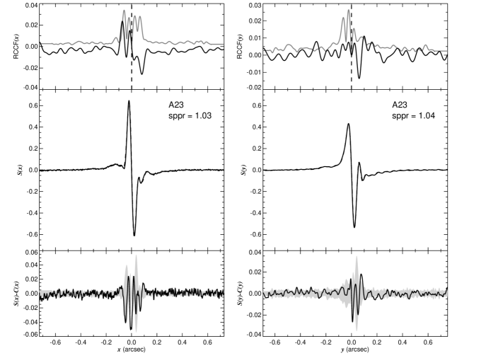
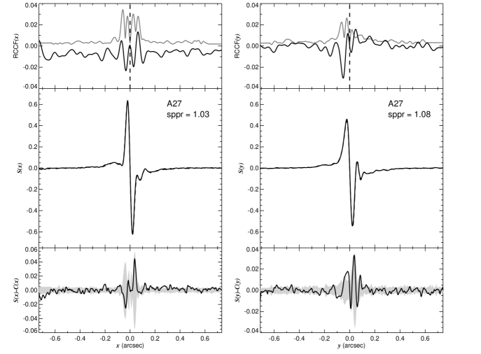
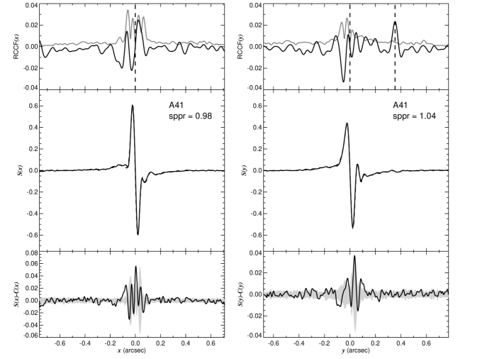
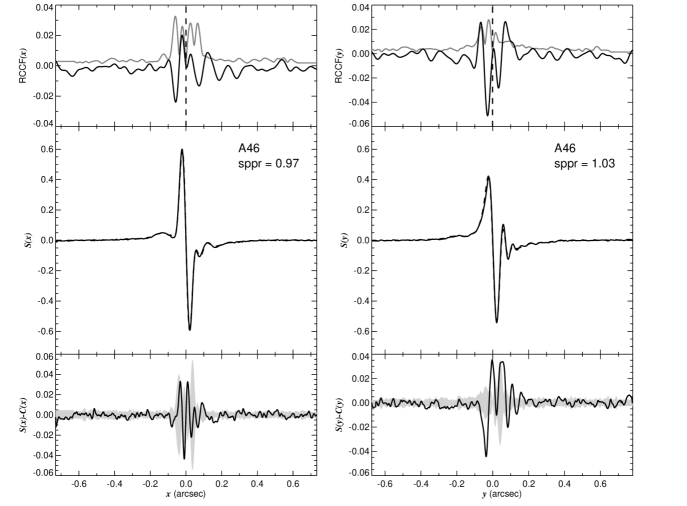
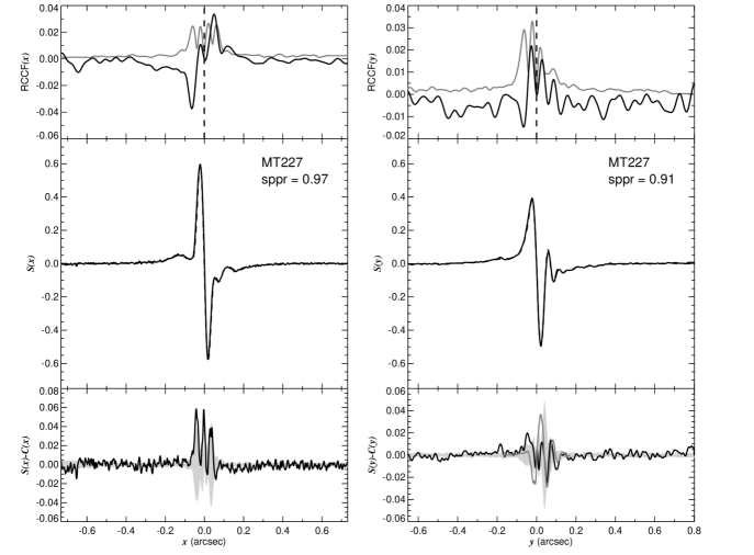
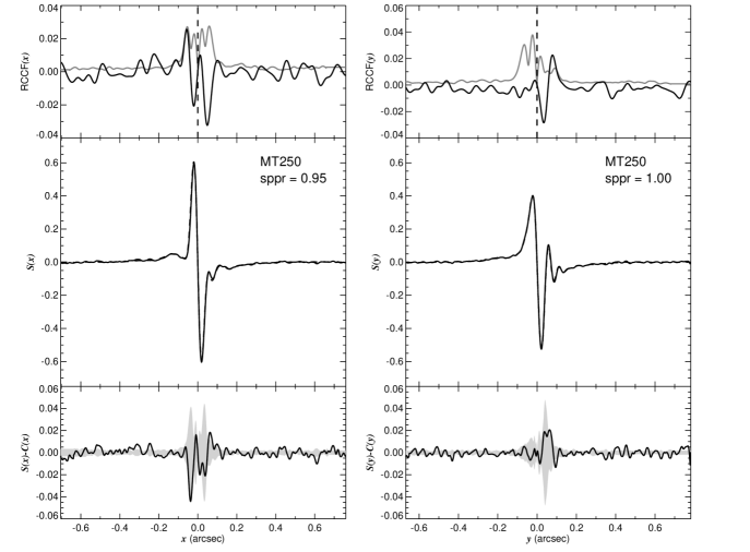
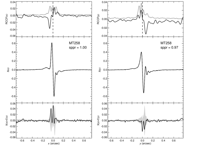
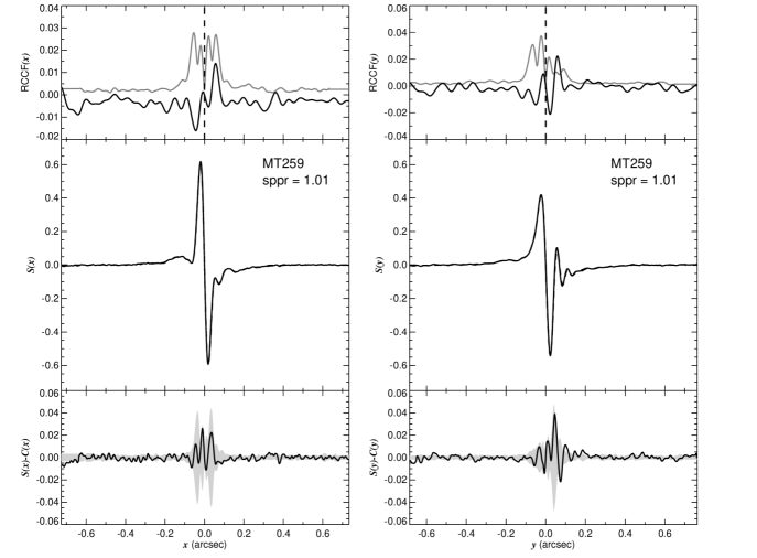
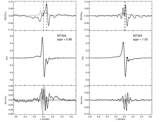
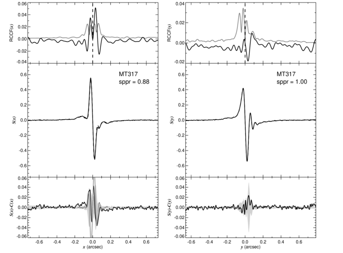
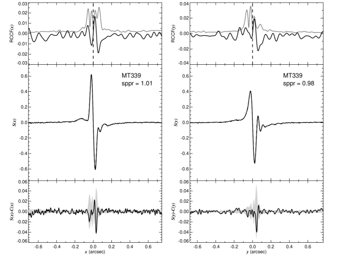
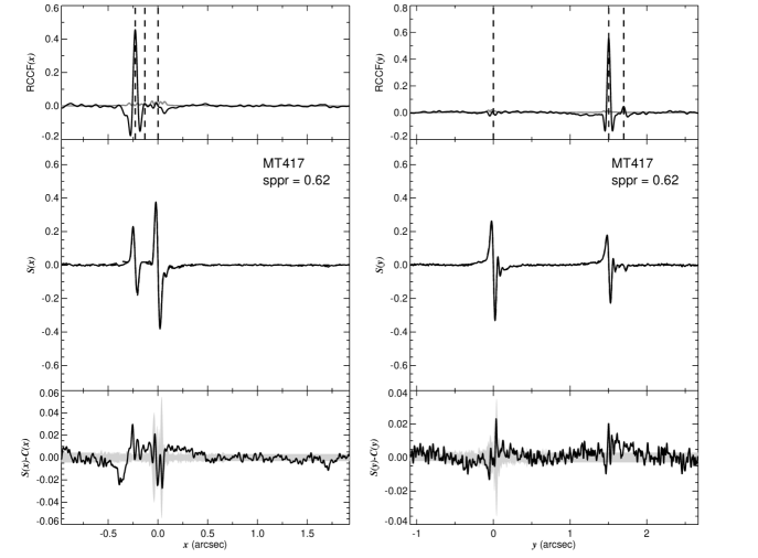
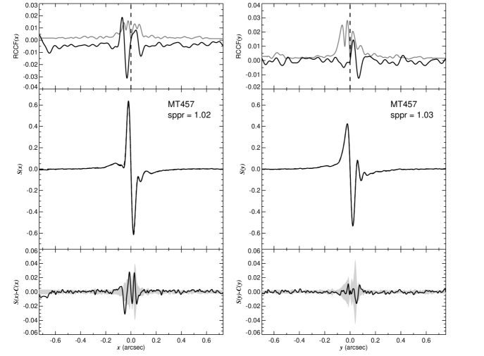
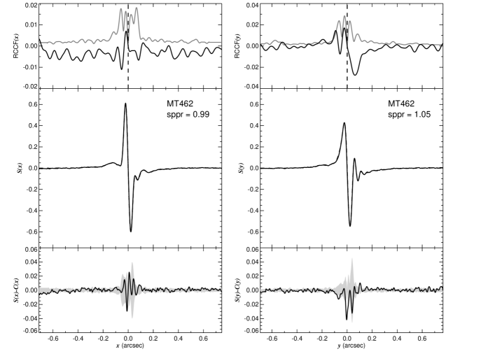
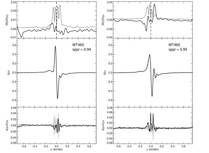
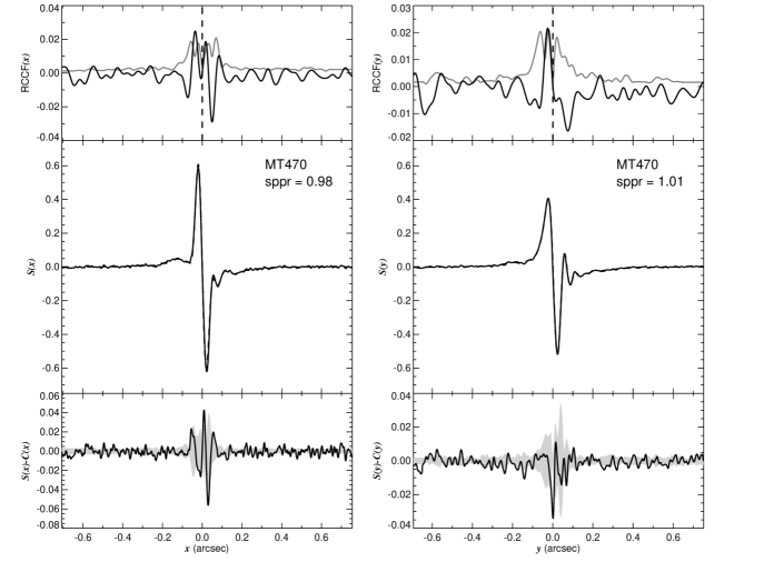
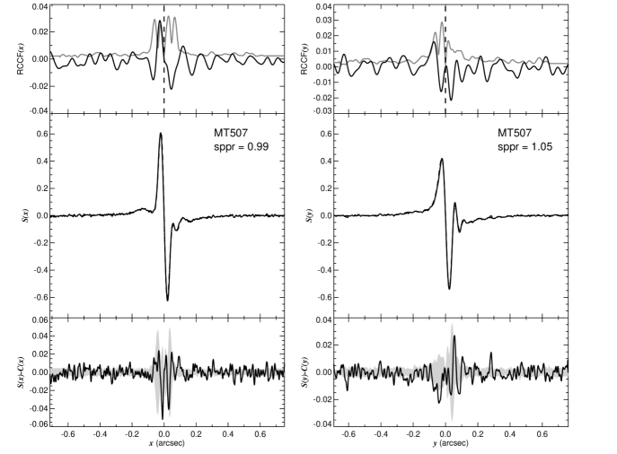
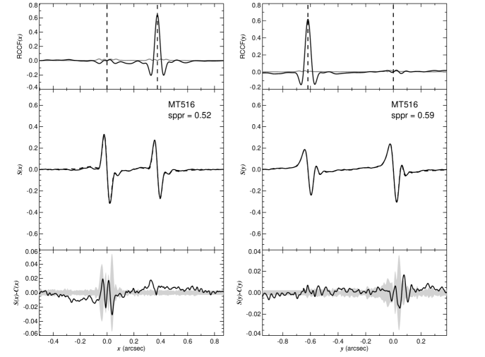
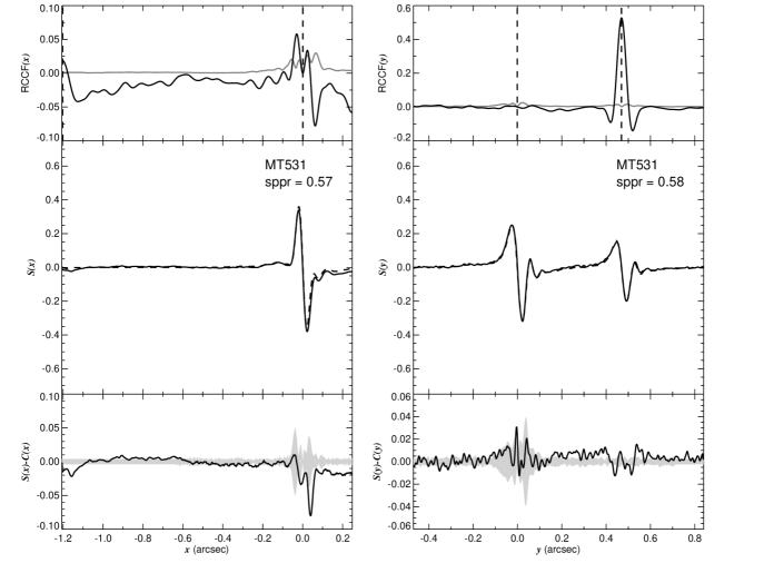
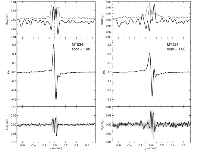
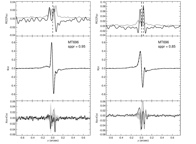
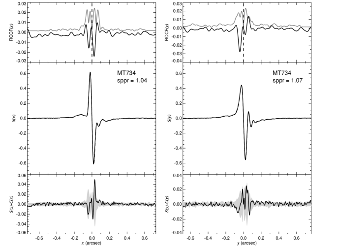
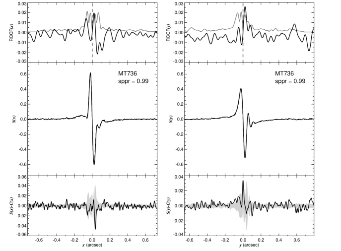
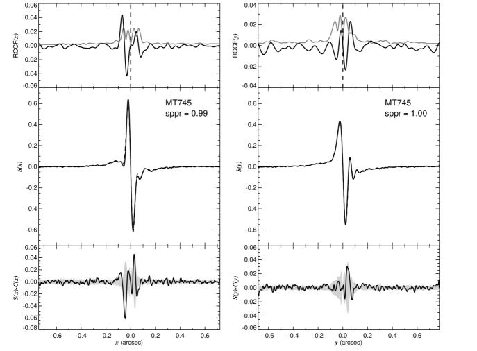
Figure Set 1 shows transfer function plots for all 58 stars in our sample. The figures show the $x$ - (left) and $y$ -axis (right) rectified $S$ -curves in the central panel. Also shown as a dashed line is a preliminary model fit based upon the components derived from the CCF analysis and the mean $S$ -curve of the calibrator set selected. The top panel plots the mean of the residual cross-correlation functions of the target with the calibrator (solid, black lines) after the peak of the primary has been subtracted off. The vertical dashed lines indicate the position of each component resolved. The solid, gray lines show the standard deviation of the residual cross-correlation functions, and a peak is considered significant only if the mean residual CCF (black) exceeds the standard deviation (gray) by four times. The bottom panels show the difference curves between the star and model calibrator $S$ -curves (solid line). The shaded, gray region is the uncertainty envelope determined from the standard deviation at each point along the $S$ -curves for the calibrators. In the case where the second derivative test resolved a blended pair (e.g. MT 304, Fig. 1.18), the second derivative of the calibrator $S$ -curve is overplotted and scaled by the $a$ coefficient (solid, gray line).

The detection threshold for a binary of a given separation is determined by comparing multiple examples of a model binary based upon the calibrator observations to the calibrator $S$ -curves. This was done using a set of 21 calibrator observations of similar color stars for both the model and calibrator curves (for a total of 420 test cases), and the faintest flux ratio was set by models that met the $4\sigma$ detection criterion. The positive (solid line) and negative (dashed line) branches are folded onto one separation axis in Figure 4 in the left and right panels for the $x$ - and $y$ -axis scans, respectively. Here the limiting flux ratio, $r$ , is shown as a magnitude difference $\Delta m=-2.5\log r$ for trial separations, and any binary brighter than the limit (i.e., below the line plots) would exceed the $4\sigma$ detection criterion. The smallest separation detected in favorable, equal flux cases is slightly better for positive separations, and the faintest detectable companions have $\triangle m=4.5$ mag at large separations. The oscillation in these curves seen near $x=y=0\farcs 06$ is due to the changing and relatively larger uncertainties in the calibrator $S$ -curves at such distances from their zero-crossing. The results in these figures compare well with the advertised limits in Figure 3.3 of the Fine Guidance Sensor Instrument Handbook (Nelan et al., 2012) except for the case of marginally resolved binaries that we discussed above.

Note that the CCF method loses its effectiveness for very close companions. The peaks in the residual CCFs in the binary models where $\rho\lesssim 25$ mas are rarely found at separations of less than $0\farcs 04$ even in favorable cases. This is due to the fact that blending of the fringe patterns becomes so severe that the calibrator CCF is positioned at the maximum that occurs between the actual positions of the components, and consequently the residual CCF shows two peaks: one for the companion and a mirror one for the primary. At the smallest separations where the method can be applied ( $0\farcs 016$ in $x$ and $0\farcs 017$ in $y$ ), the two peaks in the residual CCF approach equal intensity, and the method can no longer distinguish the direction of primary to secondary. Nevertheless, the appearance of a double-peaked feature in the residual CCF offers evidence for the presence of a marginally resolved companion that supplements the second derivative test.

The detection limits using the second derivative method were estimated by running the scheme with multiple binary models from a large sample of calibrators. The working criteria from these models for $4\sigma$ detection are $a>1.2\times 10^{-5}$ and $1.6\times 10^{-5}$ arcsec² for the $x$ - and $y$ -axes, respectively. These limits are shown in Figure 4 as dotted lines that trace the upper envelope for detection by the second derivative approach. In the best cases ( $r=1$ ), the estimates suggest that binaries as close as $0\farcs 010$ can be detected with FGS TRANS mode scans. The second derivative and CCF methods are probably both sensitive to binary detection in the $0\farcs 020$ – $0\farcs 025$ (28 – 100 AU) range.

3.4 Off-scan Components

There is also the case of very widely separated binaries, where the light of the companion falls within the instrumental FOV ( $5^{\prime\prime}\times 5^{\prime\prime}$ ), but the projected separation is greater than the length of the scan. This is the case for our observation of MT 531 where the system is resolved along the $y$ -axis, but the secondary is off the scan along the $x$ -axis (see Fig. 1.39). The CCF method will fail to detect the companion because its peak lies beyond the recorded scan. However, such binaries will still cause the $S$ -curve of the primary to appear with an amplitude reduced by a factor $\frac{1}{(1+r)}$ , and hence the ratio of target to calibrator $S$ -curve amplitude ( $sppr$ ) provides an additional criterion to check for very wide binaries. In practice, the scatter between calibrator $S$ -curves of similar color indicates that a $4\sigma$ detection may be claimed if the target $S$ -curve amplitude is less than $92\%$ of the mean calibrator $S$ -curve amplitude. Recall that overlapping fringes due to a binary may also cause the amplitude to decline, but in this case, the fringe will also be widened. Consequently, one can differentiate between the off scan and blended cases by the appearance of the difference curve. The dotted line in Figure 2 shows that the difference curve for a binary with an off-scan companion appears like a negatively scaled version of the $S$ -curve itself, which looks very different from the second derivative curve. Thus, it is important to inspect the shapes of the difference curves in order to decide if a positive detection indicates the prescence of an off-scan companion or a very close companion.

We were able to make a second check for wide companions through inspection of results from our adaptive optics (AO) survey using the Near InfraRed Imager and Spectrograph (NIRI) at the Gemini North Observatory (Caballero-Nieves, 2012). The NIRI observations have a larger dynamic range (i.e., can detect fainter companions) and have a larger field of view, so any system observed with FGS with $\rho\gtrsim 50$ mas will also be detected in the NIRI image. The infrared images allow us to identify those companions with projected separations longer than the scan length, but still within the FOV of the FGS. With the help of the NIRI observations, we were able to conclude that distant companions influence the FGS results for MT 59, MT 138 and MT 531.

4 Model Fitting

If a binary was detected, then we fit the target $S$ -curve with a model binary formed from a calibrator $S$ -curve in order to determine the relative brightness and projected separation along an axis. We used two routines to calculate the best fit model. The first is BINARY_FIT which is part of the STScI reduction package based upon algorithms developed by Space Telescope Astrometry Team at Lowell Observatory (Franz et al., 1991). In addition, we developed the Interactive Data Language (IDL) routine TRIPFIT for the special cases where BINARY_FIT was not able to converge to a satisfactory solution. Both BINARY_FIT and TRIPFIT use the $x$ and $y$ projected separations and the telescope roll angle to determine the binary separation $\rho$ and position angle $\theta$ (measured east from north).

Each binary was compared to models based upon four calibrators. The calibrators were selected to have a $B-V$ color within $\pm 0.2$ mag of the target’s color. The only exception was MT 304, with a $B-V=3.35$ , which is the reddest star in our sample by more than 1 mag. In this case we selected calibrators from the reddest, single star in our sample, MT 448, and the stars from Comerón et al. (2002) (A 23, A 27, A 41, A 46), which are red objects according to their brightness in the infrared. We adopted the fit made using the calibrator closest in color and observation date to determine the system parameters. The spread in results from fits made using the other calibrators was used to determine the fitting parameter uncertainties. The same calibrator was used to model both the primary and secondary $S$ -curves, i.e., we assumed that any color difference between the components is negligible. Our calibrator selections are indicated in column 9 of Table 1.

The program BINARY_FIT uses a least squares approach to determine the projected separation and magnitude difference of the system (Nelan & Makidon, 2011). BINARY_FIT fits scans from one axis at a time, starting from initial estimates for the projected separation along the axis and the differential magnitude. If the results for differential magnitude from the $x$ - and $y$ -axis solutions agreed within 0.2 mag, then the individual separation results were adopted as fit, but we report the magnitude difference for the axis solution with the larger separation (usually more reliable). On the other hand, if the differential magnitudes differed by more than 0.2 mag, then we adopted the value from the axis solution with the greater separation, and then re-fit the scan for the other axis by setting the adopted magnitude difference.

We encountered several cases where BINARY_FIT could not be used. (1) The fitting code is limited by the scan length of the calibrator. If the separation of the binary is larger than the scan length of the calibrator, the program is not able to recreate a binary wide enough to model properly the target. (2) BINARY_FIT only considers solutions where both components are within the scan length. For example, if the companion is recorded on one axis but lies off the scan of the other, then the program will converge to a solution of a very close system for the axis where the star is absent. (3) BINARY_FIT cannot be applied to systems with more than two components, such as the triple MT 417.

We coded the IDL program TRIPFIT to find the best fit model for triple systems using a Levenberg-Marquardt least-squares method. The program is capable of making fits of triple systems, binaries, and off-scan components. The user selects initial estimates of the positions of the components and the differential magnitudes. The program then fits the $S$ -curves one axis at a time and returns the best fit for the differential magnitudes and separations. Both BINARY_FIT and TRIPFIT return similar solutions when modeling a system. However, for most cases we adopted the results from the BINARY_FIT models because it uses the information from both axis simultaneously in determining the best fit. The cases where we could not converge on a satisfactory solution with BINARY_FIT, we report the results using TRIPFIT and those systems are noted in section 5.

There are three sources of uncertainty in the analysis of FGS data. (1) Internal errors arise from photometric shot noise, which is important for stars with $V>14$ , and spacecraft jitter that cannot be removed using the guide star centroids reported by the guiding FGSs. (2) The $S$ -curves slowly evolve over time, which is due to small changes in the alignment of the Koesters prisms relative to the optical axis of HST, made sensitive due to the spherical aberration of the HST primary mirror. By choosing calibrator stars that are observed close in time (on the order of 1 year) to the science observations this evolutionary effect is mitigated. (3) Systematic differences between the calibrators exist. To investigate how the photometric noise and jitter influence the derive parameters of a binary, we selected four binary systems (MT 5, MT 429, MT 605, and MT 632) and binned their scans into three or four independent subsets. Each subset includes approximately five scans that were shifted, co-added and smoothed using the same approach applied to the complete set of scans. The resultant subset of co-aligned scans were then fit with the best calibrator using BINARY_FIT. The small spread in the values of separation and magnitude shows that the internal error is not a significant source of uncertainty for the binary parameters (except in the case of MT 5; see section 5). Consequently, the binary parameter uncertainties are dominated by the differences between the calibrator scans, and in Table 2 we report uncertainties based upon the standard deviation of the parameter fits made with the different calibrator $S$ -curves.

5 Multiplicity Results

Table 2 lists the model fitting results for separation and differential magnitude for the 13 resolved systems in our Cyg OB2 sample. The cited errors are from a comparison of results from fits made with different calibrators as described in section 4. There were two additional cases where only the second derivative analysis indicated a possible close binary system that was partially resolved on only one axis. The derived $a$ -coefficient was $a=(15.2\pm 3.4)\times 10^{-6}$ arcsec² along the $y$ -axis for MT 227 and $a=(25.5\pm 3.6)\times 10^{-6}$ arcsec² along the $x$ -axis for MT 317. These two marginally resolved systems are objects of interest for follow-up analysis. We describe below the individual cases for the fully resolved systems.

A 41. The CCF analysis of A 41 (see Fig. 1.3) reveals the presence of a faint companion in the $y$ -axis scan. This companion was also found in the $K$ -band NIRI results at a separation of $\rho=0\farcs 35$ , essentially the same as the $y$ -axis projected separation. This implies that the companion’s projected separation along the $x$ -axis is within the fringe of the primary. This, along with its relative faintness ( $\delta V\approx 3.3$ ), make detection along the $x$ -axis challenging. Nevertheless, we fit the $S$ -curves of both axes with BINARY_FIT to obtain a separation and position angle consistent with the NIRI results.

MT 5. (see Fig. 1.5) After splitting the $S$ -curve data into subsets, the internal error was found to be a non-negligible source of uncertainty in this case. The uncertainties listed for MT 5 in Table 2 reflect both the spread among the calibrators and between the subsets of MT 5 (added in quadrature). Note that the second derivative test for the $x$ -axis ( $a=7.9\sigma$ ) indicates that the primary itself may have a close companion making this a triple system, but the test is consistent with a single primary for the $y$ -axis scan.

MT 59. TRIPFIT was used to model MT 59 (see Fig. 1.6) because the binary is too widely separated in the $x$ -axis for BINARY_FIT and because the secondary is positioned beyond the recorded scan in the $y$ -axis. In the NIRI adaptive optics image, MT 59 has a companion at $\rho=1\farcs 20$ with $\Delta K=2.75$ . This total separation is related to the projected separations by $\rho^{2}=\Delta x^{2}+\Delta y^{2}$ , so we expect that secondary would have a projected separation along the $y$ -axis of $\Delta y=-0\farcs 91$ , which is beyond the scan limits.

MT 138. We determined that MT 138 (see Fig. 1.9) is resolved along the $y$ -axis with $\Delta y=+0\farcs 066$ and $\Delta V=2.79$ mag. This magnitude difference is consistent with that from a close companion in the NIRI image at $\rho=1\farcs 5$ and $\Delta K=3.18$ mag. According to the FGS aperture position angle (or telescope roll angle), the NIRI component is expected to appear at $\Delta y=+0\farcs 070$ and $\Delta x=+1\farcs 338$ , which agrees with the BINARY_FIT result along the $y$ -axis and puts the companion well off the $x$ -axis scan.

MT 304. This target (Schulte 12 = Cyg OB2-12; see Fig. 1.18) shows evidence of a very close companion in the CCF and second derivative tests, with values of $a=8.81\sigma$ and $a=4.68\sigma$ for the $x$ - and $y$ -axes respectively. The differential magnitude from the BINARY_FIT analysis of the $x$ -axis scan was used as a constraint in the fit of the $y$ -axis scan, to arrive at $\Delta V=2.31\pm 0.21$ . For close systems, where the projected separation is less than the size of the fringe ( $\rho<15$ mas), there is an ambiguity in the “parity” of the secondary star’s position, i.e., solutions with the secondary to the left or right of the primary are indistinguishable from one another. With a separation along the $x$ -axis of $61.8\pm 3.1$ mas, and $y$ -axis solutions yielding 9.7 mas or -14.9 mas, the position angle is $283.5$ or $305.9\pm 3.3$ degrees, respectively. We were not able to detect the counterpart in the NIRI image, because the separation ( $\rho=63.6$ mas) is below the limiting resolution for NIRI ( $\approx 80$ mas), but this companion has been observed using other interferometric techniques (R. Millan-Gabet, private communication). MT 304 is an early B-type hypergiant of very high luminosity, but it may not belong to the class of Luminous Blue Variables because its flux and spectral appearance are relatively constant (Clark et al., 2012). The companion we find is too faint to alter the conclusion about the star’s high luminosity. If we assume that the projected separation corresponds to the apastron separation in a highly elliptical orbit, then the orbital period is $P\approx 30$ yr, for $M_{1}+M_{2}=120M_{\odot}$ (Clark et al., 2012) and $d=1.4$ kpc. Consequently, additional high angular resolution observations over the next few decades may lead to a mass measurement of this extraordinary star.

MT 417. This star (Schulte 22; see Fig. 1.24) is the only triple system resolved in our sample, and we developed TRIPFIT to model the scans. Visual inspection of the $y$ -axis $S$ -curve (central, right panel of Fig. 1.24) shows that there is a very faint third component near $\Delta y=+1\farcs 7$ . Comparison with the NIRI images led us to conclude that the third component fringe is blended with that of the secondary in the $x$ -axis scan. The solution for differential magnitudes for the secondary from the two axes did not agree with each other ( $\Delta m_{x}=0.85$ and $\Delta m_{y}=0.45$ ). This is due to the fact the second and third component are blended in the $x$ -axis scan, making the amplitude of the secondary’s fringe appear smaller. This is not the case for the $y$ -axis, where the two components are well separated. The value listed in Table 2 is from the $y$ -axis, which has the larger projected separation, and the error is estimated from the standard deviation between the fits of the different calibrators. MT 417 A and B have classifications of O3 If^⋆ and O6 V((f)), respectively (Sota et al., 2011). Our measurements of the Ba,Bb pair ( $\rho=0\farcs 196$ , $\theta=160^{\circ}$ , and $\Delta m=2.48$ mag) agree with previous works. The A,B pair was resolved with speckle interferometry, and on re-examining the 2007 speckle data using the methodology of Mason et al. (2009), the Ba,Bb pair were observed with $\rho=0\farcs 209$ , $\theta=180\fdg 0$ . This pair was also resolved through AstraLux and HST ACS/HRC imaging by Maíz Apellániz (2010). His positions and magnitude differences for the Ba,Bb pair ( $\rho=0\farcs 216$ , $\theta=181\fdg 48$ , and $\Delta m=2.34$ mag) agree with the speckle data and our results, within the uncertainties due to the blending of the Ba,Bb components along one axis and neglect of the spatial sensitivity of the photomultiplier tubes.

MT 429. The primary of MT 429 (see Fig. 1.25) is a short-period eclipsing binary, and the presence of the newly discovered bright third companion ( $\Delta V=1.09\pm 0.02$ ) has a strong influence on the interpretation of the radial velocity and photometric variations (Kiminki et al., 2012).

MT 516. The pair of MT 516 (see Fig. 1.38) was first resolved through speckle interferometry by Mason et al. (2009) who designate the binary as WSI 67. Our position and magnitude differences agree within the uncertainties.

MT 531. MT 531 (see Fig. 1.39) is an obvious binary in $y$ and the second component is off the scan in $x$ . The NIRI image shows the infrared counterpart with $\rho=1\farcs 45$ and $\Delta K=0.65$ mag. The NIRI position predicts that the companion has projected separation along the $x$ -axis $\Delta x=-1\farcs 38$ , well beyond the recorded scan.

MT 605. The primary of MT 605 (see Fig. 1.45) is a double-lined spectroscopic binary (Kiminki et al., 2012), and the unknown, relatively bright third companion may cause line blending difficulties for radial velocity measurements.

MT 632. This system was an obvious binary in both axes (see Fig. 1.47). We resolved the secondary in the NIRI observation and the FGS results are consistent with those from the AO measurements.

MT 696. A companion to this star (Schulte 27; Fig. 1.50) was detected using the second derivative test ( $a=8.46\sigma$ ) and the cross-correlation method for the $y$ -axis scan. (and was detected at the $3\sigma$ level in the second derivative test of the $x$ -axis scan). We adopted the differential magnitude from the $y$ -axis solution, because of the greater projected separation along the $y$ -axis. There exists a 180^∘ ambiguity in the position of the secondary along the $x$ -axis ( $\Delta x=\pm 9.7$ mas). The ambiguity is reflected in the two solutions for the position angle given in Table 2. The primary is an eclipsing, double-lined spectroscopic binary (Kiminki et al., 2012), and the presence of the FGS companion will influence the interpretation of the light curve and spectroscopy.

SCHULTE 5. This target (see Fig. 1.56) is an obvious binary in the scans of both axes. The separation is too large along the $x$ -axis for a BINARY_FIT solution, so we applied TRIPFIT to this system. The program arrived at similar results for the differential magnitude derived from the $x$ and $y$ scans, and we list the average in Table 2. The uncertainties were determined from the standard deviation between the differential magnitude from both axes. This system was first resolved by Herbig (1967). The primary is a short period ( $P=6.6$ d) eclipsing binary consisting of two luminous evolved stars (Linder et al., 2009). Kennedy et al. (2010) suggest that there is another star close to A with an orbital period of $P=6.7$ y based upon the variable radio emission. Mason et al. (2009) did not resolve the B component, probably due to the magnitude difference, but our results are consistent with recent observations by Maíz Apellániz (2010).

6 Discussion

Our high angular resolution survey of 58 massive stars in Cyg OB2 led to the detection of 13 resolved systems and the partial resolution of two other stars. The resulting binary fraction of 22% to 26% is consistent with the results from Nelan et al. (2004), who resolved 5 out of 23 OB stars (22%) in the Carina Nebula cluster. We were able to find the infrared counterpart in our NIRI observations for 11 of the resolved systems, but not for the marginally resolved pairs MT 304 and MT 696. Additional observations with ground-based interferometry confirm the companion to MT 304. Two of the most massive stars in the association (MT 304 = Cyg OB2-12 and MT 417 = Cyg OB2-22A) have resolved companions while the third very massive star (MT 457 = Cyg OB2-7) appears single. The companion of the hypergiant MT 304 (Cyg OB2-12) may have an orbital period of a few decades, and continued high angular resolution observations should reveal the companion’s orbital motion. This is potentially a very important target for mass determination (like HD 93129A; Nelan et al. 2004).

The high angular resolution capabilities of the FGS allow us to start filling in the observational gap in the period distribution of massive binaries (Mason et al., 1998). The angular separations of the resolved binaries correspond to binary orbital periods in the range of $20<P<20,000$ yrs. The longest period spectroscopic system in Cyg OB2 observed by Kobulnicky et al. (2012) is just over 6 yr, only a factor of 3 smaller than our lower limit. This is probably the smallest gap to date between spectroscopic and high angular resolution methods. Though most of our resolved companions have long periods, their projected separations are less than 10,000 AU. This corresponds to an orbital velocity that is larger than the velocity dispersion of the association ( $\sigma=8.03$ km s^-1; Kiminki et al. 2008), so these systems are probably orbitally bound companions.

The companions we detected are relatively bright, and hence, it is important to account for their flux in analyzing the spectra of the primary stars. Fainter companions are undoubtedly present in this period range, and our complementary adaptive optics study with NIRI (Caballero-Nieves et al., in prep.) will help to determine the mass ratio distribution of lower mass and fainter companions (at least among the long period binaries). The systems resolved in our sample are at the limits of what is angularly resolvable with a single aperture telescope today. Preliminary results from the larger AO sample allows us to perform a statistical study of chance alignments, which suggests that the systems resolved with the FGS have $<1$ % probability of being a chance alignment. In a future work we will combine the results of the spectroscopic and high angular resolution surveys of Cyg OB2 and provide an unprecedented census of the binary properties of massive stars over a large range in orbital period.

We thank the staff of the Space Telescope Science Institute (STScI) for their support in obtaining these observations. We are also grateful to Dr. John P. Subasavage who helped implement the FGS reduction pipeline at GSU. Support for HST proposal numbers GO-9646, 9840, and 10612 was provided by NASA through a grant from the Space Telescope Science Institute, which is operated by the Association of Universities for Research in Astronomy, Incorporated, under NASA contract NAS5-26555. This work was also supported by the National Science Foundation under grants AST-0606861 and AST-1009080. A. F. J. Moffat is grateful for financial aid from the Natural Sciences and Engineering Research Council of Canada (NSERC). Institutional support has been provided from the GSU College of Arts and Sciences and from the Research Program Enhancement fund of the Board of Regents of the University System of Georgia, administered through the GSU Office of the Vice President for Research and Economic Development. We are grateful for all this support. Facilities: HST (FGS)

References

Caballero-Nieves (2012) Caballero-Nieves, S. M. 2012, PhD thesis, Georgia State University
Caballero-Nieves et al. (in prep.) Caballero-Nieves, S. M., Gies, D. R., Baines, E. K., et al. in prep., ApJ
Chini et al. (2012) Chini, R., Hoffmeister, V. H., Nasseri, A., Stahl, O., & Zinnecker, H. 2012, MNRAS, 424, 1925
Clark et al. (2012) Clark, J. S., Najarro, F., Negueruela, I., et al. 2012, A&A, 541, A145
Close et al. (2012) Close, L. M., Puglisi, A., Males, J. R., et al. 2012, ApJ, 749, 180
Comerón et al. (2002) Comerón, F., Pasquali, A., Rodighiero, G., et al. 2002, A&A, 389, 874
Franz et al. (1991) Franz, O. G., Kreidl, T. J. N., Wasserman, L. W., et al. 1991, ApJ, 377, L17
Hanson (2003) Hanson, M. M. 2003, ApJ, 597, 957
Herbig (1967) Herbig, G. H. 1967, PASP, 79, 502
Herrero et al. (2001) Herrero, A., Puls, J., Corral, L. J., Kudritzki, R. P., & Villamariz, M. R. 2001, A&A, 366, 623
Horch et al. (2006) Horch, E. P., Franz, O. G., Wasserman, L. H., & Heasley, J. N. 2006, AJ, 132, 836
Kennedy et al. (2010) Kennedy, M., Dougherty, S. M., Fink, A., & Williams, P. M. 2010, ApJ, 709, 632
Kiminki & Kobulnicky (2012) Kiminki, D. C., & Kobulnicky, H. A. 2012, ApJ, 751, 4
Kiminki et al. (2007) Kiminki, D. C., Kobulnicky, H. A., Kinemuchi, K., et al. 2007, ApJ, 664, 1102
Kiminki et al. (2008) —. 2008, ApJ, 681, 735
Kiminki et al. (2012) Kiminki, D. C., Kobulnicky, H. A., Ewing, I., et al. 2012, ApJ, 747, 41
Knödlseder (2000) Knödlseder, J. 2000, A&A, 360, 539
Kobulnicky et al. (2012) Kobulnicky, H. A., Smullen, R. A., Kiminki, D. C., et al. 2012, ApJ, 756, 50
Kouwenhoven et al. (2007) Kouwenhoven, M. B. N., Brown, A. G. A., Portegies Zwart, S. F., & Kaper, L. 2007, Astronomy & Astrophysics, 474, 77
Linder et al. (2009) Linder, N., Rauw, G., Manfroid, J., et al. 2009, A&A, 495, 231
Maíz Apellániz (2010) Maíz Apellániz, J. 2010, A&A, 518, A1
Mason et al. (1998) Mason, B. D., Gies, D. R., Hartkopf, W. I., et al. 1998, AJ, 115, 821
Mason et al. (2009) Mason, B. D., Hartkopf, W. I., Gies, D. R., Henry, T. J., & Helsel, J. W. 2009, AJ, 137, 3358
Mason et al. (2001) Mason, B. D., Wycoff, G. L., Hartkopf, W. I., Douglass, G. G., & Worley, C. E. 2001, AJ, 122, 3466
Massey & Thompson (1991) Massey, P., & Thompson, A. B. 1991, AJ, 101, 1408
Menten et al. (2007) Menten, K. M., Reid, M. J., Forbrich, J., & Brunthaler, A. 2007, A&A, 474, 515
Muntean et al. (2009) Muntean, V., Moffat, A. F. J., Chené, A. N., & de La Chevrotière, A. 2009, MNRAS, 399, 1977
Negueruela et al. (2008) Negueruela, I., Marco, A., Herrero, A., & Clark, J. S. 2008, A&A, 487, 575
Nelan et al. (2012) Nelan, E., Fresneau, A., Holfeltz, S. F., et al. 2012, Fine Guidance Sensor Instrument Handbook, 20th edn. (Baltimore: STScI)
Nelan & Makidon (2011) Nelan, E., & Makidon, R. B. 2011, Fine Guidance Sensor Data Handbook, 4th edn. (Baltimore: STScI)
Nelan et al. (2004) Nelan, E. P., Walborn, N. R., Wallace, D. J., et al. 2004, AJ, 128, 323
Preibisch et al. (1999) Preibisch, T., Balega, Y., Hofmann, K.-H., Weigelt, G., & Zinnecker, H. 1999, New A, 4, 531
Raghavan et al. (2010) Raghavan, D., McAlister, H. A., Henry, T. J., et al. 2010, ApJS, 190, 1
Rygl et al. (2012) Rygl, K. L. J., Brunthaler, A., Sanna, A., et al. 2012, A&A, 539, A79
Sana et al. (2008) Sana, H., Gosset, E., Nazé, Y., Rauw, G., & Linder, N. 2008, MNRAS, 386, 447
Schulte (1958) Schulte, D. H. 1958, ApJ, 128, 41
Skrutskie et al. (2006) Skrutskie, M. F., Cutri, R. M., Stiening, R., et al. 2006, AJ, 131, 1163
Sota et al. (2011) Sota, A., Maíz Apellániz, J., Walborn, N. R., et al. 2011, ApJS, 193, 24
van der Hucht (2001) van der Hucht, K. A. 2001, New A Rev., 45, 135
Walborn (1973) Walborn, N. R. 1973, ApJ, 180, L35
Walborn et al. (2002) Walborn, N. R., Howarth, I. D., Lennon, D. J., et al. 2002, AJ, 123, 2754
Weigelt et al. (1999) Weigelt, G., Balega, Y., Preibisch, T., et al. 1999, A&A, 347, L15
Wright et al. (2010) Wright, N. J., Drake, J. J., Drew, J. E., & Vink, J. S. 2010, ApJ, 713, 871
Zinnecker & Yorke (2007) Zinnecker, H., & Yorke, H. W. 2007, ARA&A, 45, 481

Table 1: Cygnus OB2 Target List

Star	R.A.	Dec.	Spectral	Class.	$V$	$B-V$	Obs. Date	Calibrator	No.	Remarks
Name	(J2000)	(J2000)	Classification	Ref.	(mag)	(mag)	(BY)	Name	Comp.
(1)	(2)	(3)	(4)	(5)	(6)	(7)	(8)	(9)	(10)	(11)
A 23	20:30:39.71	+41:08:49.0	B0.7 Ib	1	11.25	$\cdots$	2007.2729	$\cdots$	1	$\cdots$
A 27	20:34:44.72	+40:51:46.6	B0 Ia	2	11.26	$\cdots$	2007.4675	$\cdots$	1	$\cdots$
A 41	20:31:08.38	+42:02:42.3	O9.7 II	1	11.70	$\cdots$	2006.0666	$\cdots$	2	NIRI
A 46	20:31:00.20	+40:49:49.7	O7 V((f))	1	11.40	$\cdots$	2008.4988	$\cdots$	1	$\cdots$
MT 5	20:30:39.82	+41:36:50.7	O6 V	3	12.93	1.64	2006.5055	WR 145	2	NIRI
MT 59	20:31:10.55	+41:31:53.5	O8 V	4	11.18	1.47	2006.4855	MT 601	2	NIRI, SB1
MT 70	20:31:18.33	+41:21:21.7	O9 II	4	12.99	2.10	2006.4928	$\cdots$	1	SB1
MT 83	20:31:22.04	+41:31:28.4	B1 I	3	10.64	1.18	2006.0001	$\cdots$	1	SB1
MT 138	20:31:45.40	+41:18:26.8	O8 I	3	12.26	1.99	2006.4854	MT 390	2	NIRI, SB1
MT 145	20:31:49.66	+41:28:26.5	O9 III	4	11.52	1.11	2005.9990	$\cdots$	1	SB1
MT 213	20:32:13.13	+41:27:24.6	B0 V	3	11.95	1.13	2007.2387	$\cdots$	1	RV constant
MT 217	20:32:13.83	+41:27:12.0	O7 IIIf	3	10.23	1.19	2006.3752	$\cdots$	1	RV constant
MT 227	20:32:16.56	+41:25:35.7	O9 V	3	11.47	1.24	2006.4883	$\cdots$	1	$\cdots$
MT 250	20:32:26.08	+41:29:39.4	B2 III	3	12.88	1.06	2007.2942	$\cdots$	1	RV constant
MT 258	20:32:27.66	+41:26:22.1	O8 V	4	11.10	1.20	2006.4986	$\cdots$	1	SB1
MT 259	20:32:27.74	+41:28:52.3	B0 Ib	3	11.42	1.00	2006.3778	$\cdots$	1	SB1
MT 299	20:32:38.58	+41:25:13.8	O7 V	3	10.84	1.19	2006.4773	$\cdots$	1	SB1?
MT 304	20:32:40.96	+41:14:29.2	B3-4 Ia⁺	5	11.10	3.35	2006.2346	MT 448	2	$\cdots$
MT 317	20:32:45.46	+41:25:37.4	O8 V	3	10.68	1.25	2006.4959	$\cdots$	1	RV constant
MT 339	20:32:50.02	+41:23:44.7	O8 V	3	11.60	1.35	2006.5004	$\cdots$	1	RV constant
MT 376	20:32:59.19	+41:24:25.5	O8 V	3	11.91	1.35	2006.4963	$\cdots$	1	RV constant
MT 390	20:33:02.92	+41:17:43.1	O8 V	3	12.95	1.98	2006.4844	$\cdots$	1	RV constant
MT 403	20:33:05.27	+41:43:36.8	B1 V	3	12.94	1.49	2007.4728	$\cdots$	1	$\cdots$
MT 417	20:33:08.80	+41:13:18.2	O3 If^⋆	6	11.55	2.04	2006.3776	MT 771	3	NIRI, SB1
MT 429	20:33:10.51	+41:22:22.5	B0 V	4	12.98	1.56	2007.2895	MT 793	2	NIRI, SB1/EA
MT 431	20:33:10.75	+41:15:08.2	O5:	4	10.96	1.81	2006.3065	$\cdots$	1	SB2
MT 448	20:33:13.26	+41:13:28.7	O6 V	3	13.61	2.15	2006.4894	$\cdots$	1	SB1
MT 455	20:33:13.69	+41:13:05.8	O8 V	3	12.92	1.81	2006.4879	$\cdots$	1	$\cdots$
MT 457	20:33:14.11	+41:20:21.8	O3 If^⋆	3	10.55	1.45	2006.3397	$\cdots$	1	RV constant
MT 462	20:33:14.76	+41:18:41.6	O7 III-II	3	10.33	1.44	2006.5006	$\cdots$	1	RV constant
MT 465	20:33:15.08	+41:18:50.5	O5.5 I	4	09.06	1.30	2006.4567	$\cdots$	1	SB2
MT 470	20:33:15.71	+41:20:17.2	O9 V	3	12.50	1.46	2006.4930	$\cdots$	1	RV constant
MT 473	20:33:16.34	+41:19:01.8	O8.5 V	3	12.02	1.45	2006.4936	$\cdots$	1	RV constant
MT 480	20:33:17.48	+41:17:09.3	O7 V	3	11.88	1.59	2006.4903	$\cdots$	1	RV constant
MT 483	20:33:17.99	+41:18:31.1	O5 III	3	10.19	1.24	2006.3069	$\cdots$	1	SB1?
MT 485	20:33:18.03	+41:21:36.6	O8 V	3	12.06	1.51	2006.4881	$\cdots$	1	SB1?
MT 507	20:33:21.02	+41:17:40.1	O9 V	3	12.70	1.54	2006.4934	$\cdots$	1	RV constant
MT 516	20:33:23.46	+41:09:13.0	O5.5 V	3	11.84	2.20	2006.3067	MT 448	2	NIRI, RV constant
MT 531	20:33:25.56	+41:33:27.0	O8.5 V	3	11.58	1.57	2006.4961	MT 480	2	NIRI, RV constant
MT 534	20:33:26.75	+41:10:59.5	O8.5 V	3	13.00	1.87	2006.4892	$\cdots$	1	RV constant
MT 555	20:33:30.31	+41:35:57.9	O8 V	3	12.51	1.90	2007.2411	$\cdots$	1	SB1
MT 556	20:33:30.79	+41:15:22.7	B1 I	3	11.01	1.77	2006.4937	$\cdots$	1	SB1
MT 588	20:33:37.00	+41:16:11.3	B0 V	3	12.40	1.66	2007.2413	$\cdots$	1	RV constant
MT 601	20:33:39.11	+41:19:25.9	B0 Iab	3	11.07	1.47	2006.2571	$\cdots$	1	SB1
MT 605	20:33:39.80	+41:22:52.4	B1 V	4	11.78	1.19	2007.2469	MT 217	2	NIRI, SB2
MT 611	20:33:40.87	+41:30:19.0	O7 V	3	12.77	1.55	2006.0664	$\cdots$	1	RV constant
MT 632	20:33:46.10	+41:33:01.1	O9 I	3	09.88	1.59	2006.4770	MT 480	2	NIRI
MT 642	20:33:47.84	+41:20:41.5	B1 III	3	11.78	1.55	2007.2442	$\cdots$	1	SB1
MT 692	20:33:59.25	+41:05:38.1	B0 V	3	13.61	1.69	2007.4677	$\cdots$	1	SB2?
MT 696	20:33:59.53	+41:17:35.5	O9.5 V	4	12.32	1.65	2007.2415	MT 588	2	SB2/EW/KE
MT 734	20:34:08.50	+41:36:59.2	O5 I	4	10.03	1.49	2006.4180	$\cdots$	1	SB1
MT 736	20:34:09.52	+41:34:13.7	O9 V	3	12.79	1.46	2007.2532	$\cdots$	1	RV constant
MT 745	20:34:13.51	+41:35:02.7	O7 V	3	11.91	1.50	2005.9724	$\cdots$	1	SB1?
MT 771	20:34:29.60	+41:31:45.5	O7 V	4	12.06	2.05	2007.2507	$\cdots$	1	SB2
MT 793	20:34:43.58	+41:29:04.6	B2 IIIe	3	12.29	1.54	2007.2505	$\cdots$	1	$\cdots$
SCHULTE 5	20:32:22.43	+41:18:19.1	O7 Ianfp	4	09.12	1.67	2006.5002	MT 588	2	NIRI, SB2/EB
SCHULTE 73	20:34:21.93	+41:17:01.6	O8 III	4	12.40	1.73	2007.2497	$\cdots$	1	SB2
WR 145	20:32:06.29	+40:48:29.6	WN7o/CE	7	11.83	1.63	2006.4932	$\cdots$	1	SB1

References. — Column 5: 1. Hanson (2003); 2. Negueruela et al. (2008); 3. Kiminki et al. (2007); 4. Kobulnicky et al. (2012); 5. Clark et al. (2012); 6. Sota et al. (2011); 7. Muntean et al. (2009).

Table 2: Multiplicity Parameters for Resolved Systems

Star	$\Delta x$	$\Delta y$	$\rho$	$\theta$	$\Delta m_{\rm F583W}$
Name	(mas)	(mas)	(mas)	(^∘)	(mag)
A 41	54.4 $\pm$ 15.2	352.6 $\pm$ 1.4	356.8 $\pm$ 3.1	276.1 $\pm$ 6.5	3.27 $\pm$ 0.86
MT 5	$-129.6\pm$ 1.4	294.0 $\pm$ 1.1	321.3 $\pm$ 0.8	91.7 $\pm$ 0.3	2.79 $\pm$ 0.09
MT 59	$-751.3\pm$ 0.8	$\cdots$	$>$ 751.3 $\pm$ 0.8	$\cdots$	2.58 $\pm$ 0.04
MT 138	$\cdots$	66.0 $\pm$ 3.1	$>$ 66.0 $\pm$ 3.1	$\cdots$	2.79 $\pm$ 0.24
MT 304	61.8 $\pm$ 3.1	( $-14.9$ or 9.7) $\pm$ 4.6	63.6 $\pm$ 3.5	(305.9 or 283.5) $\pm$ 3.3	2.31 $\pm$ 0.21
MT 417 A,Ba	$-231.3\pm$ 1.3	1505.0 $\pm$ 3.9	1522.7 $\pm$ 3.7	146.9 $\pm$ 0.5	0.45 $\pm$ 0.01
MT 417 A,Bb	$-214.1\pm$ 5.1	1700.0 $\pm$ 2.5	1715.7 $\pm$ 2.9	147.9 $\pm$ 0.4	2.66 $\pm$ 0.32
MT 429	$-36.2\pm$ 0.7	$-95.8\pm$ 0.3	101.9 $\pm$ 0.3	23.5 $\pm$ 0.4	1.09 $\pm$ 0.02
MT 516	374.5 $\pm$ 0.04	$-618.0\pm$ 0.1	722.6 $\pm$ 0.09	325.7 $\pm$ 0.1	0.28 $\pm$ 0.02
MT 531	$\cdots$	470.8 $\pm$ 0.08	$>$ 470.8 $\pm$ 0.08	$\cdots$	0.50 $\pm$ 0.04
MT 605	99.0 $\pm$ 0.15	61.2 $\pm$ 0.5	116.4 $\pm$ 0.4	255.0 $\pm$ 0.2	0.69 $\pm$ 0.02
MT 632	165.0 $\pm$ 0.3	$-144.1\pm$ 0.3	219.1 $\pm$ 0.2	247.2 $\pm$ 0.09	2.00 $\pm$ 0.16
MT 696	( $\pm$ 9.7) $\pm$ 1.5	20.6 $\pm$ 2.7	22.8 $\pm$ 3.0	(175.1 or 225.6) $\pm$ 1.9	0.94 $\pm$ 0.40
SCHULTE 5	$-801.1\pm$ 2.2	439.6 $\pm$ 2.1	913.9 $\pm$ 2.3	56.4 $\pm$ 0.11	2.93 $\pm$ 0.29

Refer to caption — Figure 1.1: The final $S$ -curves for the $x$ and $y$ orthogonal scans for A 23. The top panels show the mean residual cross-correlation functions (black line: after removal of the primary component) plus the CCF standard deviations (gray line). The positions of components are indicated by vertical dashed lines. The middle panels show the observed (solid line) and modeled (dashed line) $S$ -curves. The lower panels display the observed minus model residuals (black line) and standard deviation (gray region) plus a fit of the second derivative (gray line) if a blended companion is present.