A statistical study of gaseous environment of Spitzer interstellar bubbles

Abstract

The expansion of interstellar bubbles is suggested to be an important mechanism of triggering material accumulation and star formation. In this work, we investigate the gaseous environment of a large sample of interstellar bubbles identified by the Spitzer space telescope, aiming to explore the possible evidence of triggered gas accumulation and star formation in a statistical sense. By cross-matching 6 124 Spitzer interstellar bubbles from the Milky Way Project (MWP) and more than 2 500 Galactic H II regions collected by us, we obtain the velocity information for 818 MWP bubbles. To study the gaseous environment of the interstellar bubbles and get rid of the projection effect as much as possible, we constrain the velocity difference between the bubbles and the ¹³CO(1$-$0) emission extracted from the Galactic Ring Survey (GRS). Three methods: the mean azimuthally averaged radial profile of ¹³CO emission, the surface number density of molecular clumps, and the angular cross-correlation function of MWP bubbles and the GRS molecular clumps are adopted. Significant over density of molecular gas is found to be close to the bubble rims. 60% of the studied bubbles were found to have associated molecular clumps. By comparing the clump-associated and the clump-unassociated MWP interstellar bubbles, we reveal that the bubbles in associations tend to be larger and thicker in physical sizes. From the different properties shown by the bubble-associated and bubble-unassociated clumps, we speculate that some of the bubble-associated clumps result from the expansion of bubbles. The fraction of the molecular clumps associated with the MWP bubbles is estimated to be about 20% after considering the projection effect. For the bubble-clump complexes, we found that the bubbles in the complexes with associated massive young stellar object(s) (MYSO(s)) have larger physical sizes, hence the complexes tend to be older. We propose that an evolutionary sequence might exist between the relative younger MYSO-unassociated bubble-clump complexes and the MYSO-associated complexes.

1 Introduction

Massive stars have significant dynamical influences on the ambient molecular clouds (MCs) by several feedback mechanisms, i.e. H II regions, outflows, stellar winds, jets, and supernovae explosions, among which the expansion of H II regions is suggested to be one of the most important factors (Matzner, 2002; Dale et al., 2012b). The expanding H II regions reshape the surrounding interstellar medium and may trigger the star formation (SF) (e.g. Watson et al., 2008; Deharveng et al., 2010; Thompson et al., 2012). These effects are predicted in theories and searched in observations.

Theoretically, several mechanisms of triggering star formation by H II regions have been proposed. Two major mechanisms are the “collect & collapse” process (Elmegreen & Lada, 1977) and the “radiation driven implosion” (or “radiation driven compression”) of pre-existing dense molecular clumps (Lefloch & Lazareff, 1994; Deharveng et al., 2010). Other mechanisms such as ionizing radiation acting on MCs with turbulent gas (Elmegreen et al., 1995) and dynamical instabilities of ionizing front (Garcia-Segura & Franco, 1996) have also been discussed. These mechanisms do not conflict with each other, and can work simultaneously in a single H II region (Deharveng et al., 2005).

Observationally, evidence for triggered SF by the expansion of H II regions was searched by studying the distribution of neutral material, young stellar objects (YSOs), and also the ages of molecular clumps or YSOs related to their associated H II regions. Recently, such topic has extensively benefited from the release of a large number of interstellar bubbles discovered in the Spitzer/GLIMPSE survey (Churchwell et al. 2006, 2007, hereafter CH06&07; Simpson et al. 2012). A Spitzer interstellar bubble is clearly characterized by its ring- or arc-shaped structure shown in the GLIMPSE 8 $\mu$m image. The 8 $\mu$m band of Spitzer$-$IRAC is dominated by the emission from the polycyclic aromatic hydrocarbon (PAH) molecules or clusters of molecules (Watson et al., 2008). These species are excited by absorbing the far-UV photons leaking from the central ionized gas. Hence, their emissions trace the ionizing fronts of H II regions. The 8 $\mu$m ring- or arc-shaped structure encircles the 24 $\mu$m emission features tracing the hot dusts embedded in the ionized gas (Watson et al., 2008), and also encircles the radio free-free emission features indicating the central ionized gas (see e.g., the Fig.3 of Deharveng et al., 2010). Hence, the observational properties of the Spitzer interstellar bubbles are in good agreement with that of expanding H II regions (Deharveng et al., 2010). By visual identification of YSO(s) and neutral material near the interstellar bubbles, the possible evidences of triggered SF and/or material accumulation were reported towards several individual sources, e.g. bubbles N 10 and N 49 (Watson et al., 2008; Zavagno et al., 2010; Dirienzo et al., 2012), H II region RCW 120 (Deharveng et al., 2009), and star forming region M 17 (Povich et al., 2009). Similar studies were made towards some other targets, i.e. W 51A (Kang et al., 2009), G45.45+0.06 (Paron et al., 2009), RCW 79, RCW 82, RCW 120 (Martins et al., 2010), RCW 34 (Bik et al., 2010), bubble N 65 (Petriella et al., 2010), S 51 (Zhang & Wang, 2012a), N 22 (Ji et al., 2012; Sherman, 2012), Sh2-294 (Samal et al., 2012), N 68 (Zhang & Wang, 2013), N 14 (Sherman, 2012; Dewangan & Ojha, 2012), N 74 (Sherman, 2012), N 131 (Zhang et al., 2013), G041.10$-$0.15, G041.91$-$0.12, N 80, N 91, N 92 (Dirienzo et al., 2012), N 4 (Li et al., 2013) and Sh2-284 (Puga et al., 2009). However, as pointed out by Thompson et al. (2012), these methods are almost impossible to diagnose the origin of the identified YSOs. Because it is always hard to distinguish the real physical association from the projection effect. Furthermore, with a single time observational data towards one system, it is also very difficult to exclude the possibility that some or even all of the identified YSO(s), protostar(s) and molecular clump(s) were formed spontaneously without any influences of triggering. As shown by the simulation of Dale et al. (2012a), the association of stars with the shell or pillar-like structures in the gas is a good but not a predominant indication of triggering.

Besides the investigations on individual objects, statistical studies of the correlations between large samples of YSOs or gases with interstellar bubbles provide a different prospect and shed light on inferring the presence of triggering in a statistical sense. Thompson et al. (2012) first made a statistical study of the massive star formation around 322 interstellar bubbles from CH06&07. Using the massive YSOs (MYSOs) identified from the Red MSX Source (RMS) survey (Urquhart et al., 2008), they found a significant over density of MYSOs near the bubble rims. Kendrew et al. (2012) made a similar analysis by using a more complete bubble catalogue from the Milky Way Project (MWP) (Simpson et al., 2012). They found a strong positional correlation of the RMS MYSOs/H II regions with bubbles at angular distances less than two effective bubble radii. Both of the two studies imply that a significant fraction of YSOs projectively associated with the bubble rims are likely triggered by the expansion of the bubbles/H II regions. To confirm this hypothesis, a statistical study on the gaseous environment of the interstellar bubbles is definitely needed.

Other than the distribution of YSOs around the bubbles, the observational evidence for triggered SF and material accumulation should be also present for neutral gases. The obstacle in such studies, as mentioned above is how to solve the projection effect in distinguishing the true association between the interstellar bubbles and the gaseous components. Previous efforts concentrated on visual inspection of channel maps of the observed molecular lines toward individual bubbles, through which morphological similarities between the bubbles and the ambient gas are expected. A better solution that we propose in this work might be taking the velocity information into account, since similar line-of-sight velocities of a bubble and its physically associated gas components are expected. Such attempt in a statistical sense now becomes available due to the presence of the 5 106 Spitzer interstellar bubbles identified by the MWP (Simpson et al., 2012), the largest catalogue of about 2 500 Galactic H II regions with velocity measurements compiled by us (Hou & Han 2013, in prep., to be submitted) and the publicity of a number of surveys of molecular gas (e.g. Dame et al., 2001; Jackson et al., 2006). We aim to statistically investigate the gaseous environment of the interstellar bubbles and explore the possible evidence of triggered material accumulation and star formation related to the bubbles. This work is organized as follows: In Sect. 2, we introduce the data sets of the interstellar bubbles and the molecular gas. In Sect. 3, the gaseous environment of bubbles are explored by three different methods. Discussions and conclusions are given in Sect. 4 and Sect. 5, respectively.

2 Data

To statistically study the gaseous environment of the interstellar bubbles and get rid of the projection effect as much as possible, a large sample of bubbles with line-of-sight velocity information and a systematic survey of molecular gas with appropriate resolution and sampling are needed.

2.1 Spizter interstellar bubbles with velocity information

The interstellar bubble catalogue adopted in this work is from the recently released Milky Way Project (Simpson et al., 2012), containing 5 106 bubbles identified by visual inspection of the Spitzer/GLIMPSE (Benjamin et al., 2003) and MIPSGAL (Carey et al., 2009) survey images. This catalogue has a sky coverage of $|l|<65^{\circ}$ and $|b|<1^{\circ}$. It increases the number of known interstellar bubbles (Churchwell et al., 2006, 2007) by nearly an order of magnitude. Because the observational properties of the Spitzer interstellar bubbles are in good agreement with that of expanding H II regions (Deharveng et al., 2010), to obtain the velocity information of the bubbles, we rely on the cross match between the bubbles and the H II regions whose line measurements (e.g. radio recombination lines, molecular lines) have been made.

Figure 1: Projected distribution of bubbles (red circles) on the Galactic plane. Background is an “intensity” distribution of spiral tracers (see Hou et al., 2009; Hou & Han, 2013, for a detail). Two stars represent the location of the Sun (x = 0.0 kpc, y = 8.3 kpc) and the Galactic center (x = 0.0 kpc, y = 0.0 kpc). A flat rotation curve with R₀ = 8.3 kpc and $\theta_{0}$ = 239 km s^-1 is used to calculate the kinematic distances if no photometric or trigonometric distances are available. The error bars are estimated by considering a velocity uncertainty of $\pm$ 7 km s^-1 if no errors are given by the trigonometric or photometric observations.

Figure 2: Distributions of bubble distances to the Galacitic center (left panel) and to the sun (middle panel). Right panel: Distribution of the physical effective radius of bubbles. A flat rotation curve with R₀ = 8.3 kpc and $\theta_{0}$ = 239 km s^-1 is used to calculate the kinematic distances if no photometric or trigonometric distance is available.

Aiming at illustrating the spiral structure of the Milky Way, Hou et al. (2009) compiled a large sample of Galactic H II regions. By collecting the new measurements released since then, a catalogue including about 2 500 Galactic H II regions and confident candidates with more than 4 300 line measurements is compiled (Hou & Han 2013, in prep.). It is by far the largest sample of Galactic H II regions with velocity and distance information. 1 677 of them fall within the sky coverage of the MWP.

A cross match is first made between the MWP interstellar bubbles and the Galactic H II regions. If the angular separation between a bubble and an H II region is less than one effective radius of the bubble, they are taken as coincident. 818 out of the 5 106 MWP bubbles were finally found to have matched H II regions (see details, e.g. coordinates, velocities in Table A). Among them, 721 H II regions have published distances. This number is nearly four times larger than previously known (189 in Kendrew et al., 2012). We directly assign the distance to a bubble if its corresponding H II region has a photometric or trigonometric distance. Otherwise, their published kinematic distances are re-calculated based on the new parameters: first, we modify the V_LSR according to the new solar motions (U₀ = 10.27 km s^-1, V₀ = 15.32 km s^-1 and W₀ = 7.74 km s^-1, Schönrich et al., 2010), the new values of R₀ = 8.3 kpc and $\theta_{0}$ = 239 km s^-1 are then used for a flat Galactic rotation curve (Brunthaler et al., 2011).

The distribution of the 721 MWP bubbles whose distances are obtained from their associated H II regions is presented in Fig. 1. They spread throughout the Galactic plane. The distances to the Galactic center of the 721 bubbles peak around 6 kpc (Fig. 2, left panel). Their distances to the Sun range from 0.5 kpc to $\sim$ 20 kpc with two peaks at $\sim$ 4 kpc and $\sim$ 10 kpc (Fig. 2, middle panel). Less bubbles are found with distances around $\sim$ 7 kpc from the Sun. Because the kinematic distance ambiguity problem is hard to solve. We calculated the physical effective radius for each bubble and found most of them are less than 5 pc (Fig. 2, right panel).

2.2 Survey data of molecular gas

As shown in Sect. 2.1, the selected MWP bubbles are concentrated in the inner Galactic plane. We measured the mean apparent effective radius of these bubbles to be about 2$\arcmin$. Therefore, in order to explore the gaseous environment of these bubbles, a systematic survey of molecular line(s) covering the inner Galaxy with sufficient angular resolution (better than 2$\arcmin$) and sampling is required.

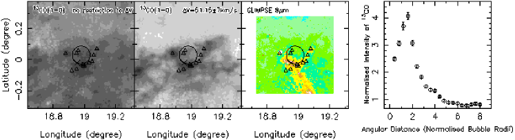
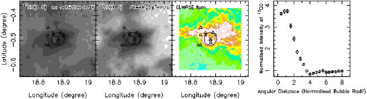
Figure 3: Upper left: velocity integrated maps of ¹³CO(1-0) for the interstellar bubble MWP1G018980+000304. The integration is performed for all the velocity range of ¹³CO(1-0) (Left first), and for the bubble-associated velocity range only (Left second). Left third: the GLIMPSE 8 $\mu$m map for the same observed regions. Upper right: normalised intensity of ¹³CO(1-0) emission as a function of the angular distance to the bubble center (see Sect. 3.1 for a detail). The error bars are estimated via the standard error of the mean. In the upper left images, the black circles indicate the apparent size of the bubble measured by the effective radius (Simpson et al., 2012). The black crosses show the central position of RRL observations. The black triangles indicate the molecular clumps identified by Rathborne et al. (2009). Lower panels: the same as upper panels, but for the interstellar bubble MWP1G018879$-$004949.

The molecular gas in our Milky Way has been widely studied by the efforts of the Columbia Galactic survey of ¹²CO (Dame et al., 2001, and reference therein), the UMASS Stony-Brook (UMSB) survey of ¹²CO (Sanders et al., 1986), the NANTEN Galactic plane survey of ¹²CO (Mizuno & Fukui, 2004), the FCRAO ¹²CO survey of the Outer Galaxy (Heyer et al., 1998), the Bell Laboratories survey of ¹³CO (Lee et al., 2001), and the Galactic ring survey of ¹³CO (Jackson et al., 2006, hereafter the GRS). The Columbia survey covers the entire Galactic plane, but the beam size is as coarse as 8.7$\arcmin$. The UMSB survey covers the first Galactic quadrant with a beam size of 45^′′, but the sampling is 3$\arcmin$. The FCRAO survey of the Outer Galaxy and the NANTEN survey do not overlap with the Spitzer/GLIMPSE survey. The Bell-Lab survey covers the first Galactic quadrant, but the angular resolution (103^′′) and the sampling (3$\arcmin$) are not qualified.

The GRS covering the Galactic longitude range from 18^∘ to 55.7^∘ and the latitude range of $|b|\leqslant$ 1^∘ meets our requirements by having an angular resolution of 46^′′ and a sampling of 22^′′. Additionally, the smaller optical depth of ¹³CO(1-0) performs as a much better tracer of the column density than ¹²CO(1-0) and results in narrower line widths, making it possible to separate the blended lines from distinct clouds with close velocities (Jackson et al., 2006). Furthermore, the GRS data of ¹³CO(1-0) have been well explored. Rathborne et al. (2009) identified 829 molecular clouds (with sizes of 20$-$60 pc) and 6 124 molecular clumps (with sizes of 3$-$20 pc) by using its data.

In the sky coverage of the GRS, 362 interstellar bubbles with associated HII regions remain, and 346 out of the 362 bubbles have known distances. The 362 bubbles and the ¹³CO survey data of the GRS, constitute the basis of our following statistical study.

3 The gaseous environment of Spitzer interstellar bubbles

To study the gaseous environment of the Spitzer interstellar bubbles, the first step is to extract the gas components which are truly associated with the bubbles. However, it is not straightforward, because the observed spectra of ¹³CO(1-0) toward a bubble are always contaminated by the emission of foreground/background molecular gas. As discussed in Sect. 2.1, the line-of-sight velocity of a bubble V_bub is taken as that of the correlated H II region. A similar velocity is expected for the associated gas components encompassing the bubble. In this work, we take $\delta$V = 7 km s^-1 as the allowance, which is a commonly adopted value for the velocity uncertainty of massive star forming regions in the Galaxy. The ¹³CO emissions with velocity between V_bub-$\delta$V and V_bub+$\delta$V were integrated, and taken as the gas components associated with the bubbles. Different values ($\delta$V = 9 km s^-1 and $\delta$V = 5 km s^-1) are also used for the calculation. We found negligible differences in the conclusions by the following statistical analysis.

To show the advantage by constraining the velocity difference between the bubbles and the gas components to solve the projection effect, we compare the results calculated by the integration of the gas components through the whole velocity range and our defined “bubble-associated” range in Fig. 3. The result implies the necessity. The two panels at the top left corner are for the bubble MWP1G018980+000304, and the two panels at the lower left corner are for the bubble MWP1G018879$-$004949. It is obvious that, after making the constraint, the features shown in the velocity integrated maps of ¹³CO(1-0) are better agreed with the arc-shaped morphology of the bubbles (see the GLIMPSE 8$\mu$m map in the left third panels.

3.1 The mean azimuthally averaged radial profile of molecular gas

The gas distribution around the Spitzer interstellar bubbles is first investigated by the azimuthally averaged radial profile of molecular gas. The profile is calculated as follows. With respect to the bubble center, the surrounding regions are separated into many rings with equal radial size. For each ring, the mean surface intensity and its standard error are calculated and normalised to the mean surface intensity of ¹³CO emission between the angular distances of two to eight effective bubble radii. The angular distance relative to the bubble center is expressed in units of the effective radius of the bubble. Hence, for the uniformly distributed molecular gas, the derived normalised intensity of ¹³CO emission is equal to 1, whatever the angular distance is. For the non-uniform distribution, the higher value of the normalised intensity, the higher degree of the gas accumulation at the corresponding position(s).

The calculated azimuthally averaged radial profiles for the bubbles MWP1G018980+000304 and MWP1G018879$-$004949 are shown as examples in the right two panels of Fig. 3. The profile for MWP1G018980+000304 peaks at $\sim$ 1.5 effective bubble radii, while that for the bubble MWP1G018879$-$004949 is at $\sim$ 1.0 effective bubble radius. These results reveal that the over density of molecular gas is close to the boundaries of the two bubbles.

The same calculations were then applied to all of the 362 MWP bubbles which have been selected in Sect. 2.2. However, some bubbles have to be discarded since the velocity coverage of the GRS spectra is from $-$5 km s^-1 to 135 km s^-1, out of the selection criteria (between V${}_{bub}-$ $\delta$V and V${}_{bub}+$ $\delta$V). Some other bubbles are located close to the boundary of the GRS sky coverage, their azimuthally averaged radial profiles cannot be derived at larger angular distances. Hence, they were also skipped. Finally, we obtained the azimuthally averaged radial profiles for 309 MWP bubbles in total. They were then averaged to generate the mean molecular gas profile of the interstellar bubbles, as presented in Fig. 4. For comparison, the mean profile for a random sample of 3 090 bubbles (ten time larger in quality than that of the selected MWP bubbles) is shown in the same plot. The random sample is not from any real measurements, but generated artificially. The parameters (effective radius, coordinates and velocity) of the random sample are randomly created, but constrained to have similar distributions of the effective radius, coordinates and velocity to those of the 309 MWP bubbles.

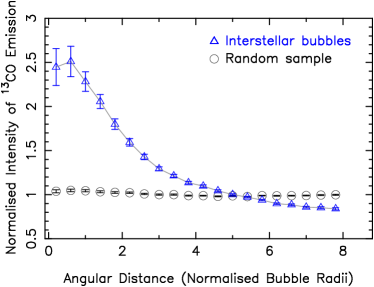
Figure 4: Mean azimuthally averaged radial profiles of molecular gas for the 309 MWP bubbles (open triangles) and for the random sample (open circles). Error bars are estimated via the standard error of the mean.

A clear excess in the normalised intensity of ¹³CO at angular distances less than about three effective bubble radii is visible. A peak appears at angular distance of about one effective bubble radius, indicating the presence of gas over density in the immediate periphery of the bubbles. At larger angular distances, the normalised intensity of ¹³CO gradually falls and reaches the values close to 1. In comparison, the mean profile always stays around 1 for the random sample. It implies that the gas component is non-uniformly distributed around the MWP interstellar bubbles. The intensity is statistically higher-than-average at smaller effective bubble radii, especially for the regions close to the bubble rims, and at larger angular distances, the intensity is much lower. This result for the gas component resembles the projected distribution of MYSOs around the interstellar bubbles found by Thompson et al. (2012) and Kendrew et al. (2012).

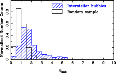
Figure 5: Distributions of $\eta_{bub}$ for the 309 MWP bubbles (blue) and the random sample (black), where $\eta_{bub}$ is the ratio of the normalised intensity of ¹³CO integrated between the angular distances of 0.5 and 2.0 effective bubble radii to that between 6.0 and 7.5 effective bubble radii.

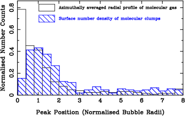
Figure 6: Distributions of the peak positions of the azimuthally averaged radial profile (black) and the surface number density of molecular clumps (blue) for the 309 MWP Bubbles.

We note that the averaged profile places emphasis on showing the mean statistical properties of the gas distribution for the overall bubbles, but loses sight to individual bubble. Therefore, we calculate the accumulation parameter $\eta_{bub}$, which is defined as the ratio of the normalised ¹³CO intensity integrated between the angular distances of 0.5 and 2.0 effective bubble radii to that between 6.0 and 7.5 effective bubble radii. The larger the $\eta_{bub}$, the higher degree of the gas accumulation near the bubble. Fig. 5 shows that the gas accumulation degree is diverse in bubbles. 187 ($\sim$61%) bubbles are found with $\eta_{bub}$ $>$ 1.5. We present the distribution of the peak position in Figure 6. Although the majority peak at angular distances less than two effective bubble radii, some do have peaks at larger angular distances, indicating the gas over density at the periphery of the interstellar bubbles does not occur in every case.

3.2 The surface number density of molecular clumps

The azimuthally averaged radial profile reveals the statistical over density of molecular gas near the bubble rims. However, the dense molecular gas concentrates in molecular clumps, hence the calculation of the mean surface intensity dilutes these structures and may underestimate the significance. 6 124 molecular clumps with ¹³CO emission in the GRS have been identified by Rathborne et al. (2009). This enables us to make a statistical study of the distribution of molecular clumps around the bubbles.

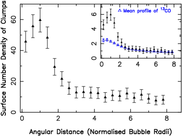
Figure 7: Surface number density of molecular clumps as a function of the effective bubble radii. Error bars are determined via Poison statistics. The mean azimuthally averaged radial profile of molecular gas (blue, see Fig. 4) is compared in the inset.

As the method described above, the “bubble-associated” clumps were first selected out by the velocity criteria of $\delta V=7$ km s^-1. Then instead of calculating the mean radial intensity of ¹³CO ring by ring, we estimated the surface number density of clumps in each ring area (number count of clumps divided by the ring area). The average distribution for all the 309 investigated bubbles is shown in Fig. 7. Prominent excess appears at angular distances less than two effective bubble radii. A significant peak is found near one effective bubble radius at about 7.7 $\sigma$ level. The surface number density of clumps falls sharply from one effective bubble radius to larger angular distances, and reaches a background value of about 10 clumps per unit area. In the inset of Fig. 7, we divide the surface number density by the background value of 10, and compare with the result calculated by the method of the azimuthally averaged radial profile shown in Fig. 4. Obviously, the peak revealed by the surface number density method is more pronounced.

Similar with the analysis in Sect. 3.1, we define an accumulation parameter $\rho_{bub}$ as the ratio of the surface number density of molecular clumps between the angular distances of 0.5 and 2.0 effective bubble radii to that between 6.0 and 7.5 effective bubble radii. The distribution of $\rho_{bub}$ is shown in Fig. 8. 60% of the bubbles are found with $\rho_{bub}>$ 1.5 and some of the bubbles has accumulation parameter $\rho_{bub}<$ 0.5, indicating barely no associated molecular clumps can be identified in the GRS data. The peak position of the surface number density of molecular clumps is calculated and compared in Fig. 6.

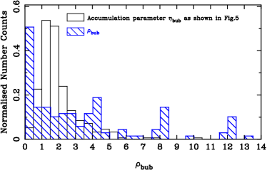
Figure 8: Distribution of the accumulation parameter $\rho_{bub}$ for the bubbles (blue), where $\rho_{bub}$ is the ratio of the surface number density of molecular clumps between the angular distances of 0.5 and 2.0 effective bubble radii to that between 6.0 and 7.5 effective bubble radii. The accumulation parameter $\eta_{bub}$ for the azimuthally averaged radial profile of molecular gas is compared (black, see Fig. 5 and Sect.3.1).

3.3 The cross-correlation of MWP bubbles and GRS molecular clumps

The surface number density of molecular clumps overcomes the dilution of gas accumulation led by the method of radial intensity profile and confirms the gas over density around the bubble rims. To learn the uncertainty and the significance of the over density more independently, we further check the angular cross-correlation function of the MWP bubbles and the GRS molecular clumps.

To calculate the angular cross-correlation function, we adopt the Landy-Szalay estimator (Landy & Szalay, 1993):

$$\omega(\theta)=\frac{N_{DD}(\theta)-2N_{DR}(\theta)+N_{RR}(\theta)}{N_{RR}(\theta)},$$ (1)

where $\theta$ is the angular separation between two objects, N${}_{i,j}(\theta)$ ($i$ = $D$ or $R$, $j$ = $D$ or $R$) is the normalised number of pairs between sample $i$ and sample $j$ with angular separation of $\theta$. Subscripts $D$ and $R$ represent the data sample and the random sample, respectively. For two different data sets, Eq. 1 can be modified to:

$$\omega(\theta)=\frac{N_{D_{1}D_{2}}(\theta)-N_{D_{1}R_{1}}(\theta)-N_{R_{1}D_{2}}(\theta)+N_{R_{1}R_{2}}(\theta)}{N_{R_{1}R_{2}}(\theta)},$$ (2)

as in Bradshaw et al. (2011), Thompson et al. (2012) and Kendrew et al. (2012). In this work, the subscripts $D_{1}$ and $D_{2}$ indicate the MWP bubble and the GRS molecular clump sample, respectively. The subscripts $R_{1}$ and $R_{2}$ indicate the random samples for the bubbles and molecular clumps.

In matching the pairs between the bubbles and the clumps, we only consider the objects whose velocity difference is less than $\delta V=7$ km s^-1. The random sample of the bubbles is randomly generated, but with similar distributions of coordinates, velocity and effective radius to those of the 309 MWP bubbles, and 32 times larger in quantity. The random sample of the molecular clumps was generated the same way to those of the 6 124 GRS molecular clumps. The bootstrap re-sampling was used to estimate the errors. 100 bootstrap iterations were made in our analysis.

Figure 9: Angular cross-correlation function $\omega$($\theta$) for the MWP bubbles and the GRS molecular clumps. The error bars were estimated by the method of bootstrap re-sampling, and given at the 1$\sigma$ level.

We show the cross-correlation result of the MWP bubbles and the GRS molecular clumps in Fig. 9. Similar features are found to that derived by the surface number density of molecular clumps. A pronounced peak at 9.2$\sigma$ level appears near one effective bubble radius. There is a prominent excess of the angular cross-correlation function $\omega$($\theta$) at the angular distances less than about two effective bubble radii, implying that the probability of finding the GRS molecular clumps around the bubble rims is significantly higher than in the outer regions. At angular distances larger than about three effective bubble radii, $\omega$($\theta$) stays around 0.0, indicating that the molecular clumps at larger distances are not correlated with bubbles.

Possible intrinsic clustering of molecular clumps at a scale close to the typical angular sizes of the bubbles could contaminate the estimates of the over density of molecular clumps near the bubble rims. We inspect this effect as Thompson et al. (2012) and Kendrew et al. (2012). The 6 124 GRS molecular clumps are separated into two sub-samples. Sub-sample 1 contains 3 068 clumps lying outside three effective bubble radii of any of the 5 106 MWP bubbles and that are essentially unassociated with any bubbles. Sub-sample 2 contains the bubble-associated clumps, which includes 492 molecular clumps lying within two effective bubble radii from one of the 309 MWP bubbles, and having velocity difference less than $\delta V=7$ km s^-1. The auto-correlation functions (see Eq. 1) for the full sample of the GRS molecular clumps, sub-sample 1 and sub-sample 2 were calculated and presented in Fig. 10.

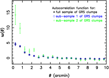
Figure 10: Results of autocorrelation functions $\omega$($\theta$) for the full sample of the GRS molecular clumps (black filled triangles), the sample of the bubble-unassociated clumps (sub-sample 1, blue open circles) and the bubble-associated clumps (sub-sample 2, green open squares).

Table 1: Properties for the clump/MYSO-associated and unassociated MWP bubbles. The T-statistic significance for the properties of the clump-associated/-unassociated and MYSO-associated/-unassociated bubbles are given in Column (3) and (6), respectively. A small value of the significance indicates that the two investigated samples have significantly different means.

		clump-associated	clump-unassociated	T-statistic	MYSO-associated	MYSO-unassociated	T-statistic
		bubbles	bubbles	significance	bubbles	bubbles	significance
		(1)	(2)	(3)	(4)	(5)	(6)
mean effective radius
	apparent (arcmin)	1.49 $\pm$ 0.08	0.89 $\pm$ 0.06	$<$ 0.1%	1.41 $\pm$ 0.12	1.15 $\pm$ 0.05	1.8%
	physical (pc)	2.90 $\pm$ 0.18	2.26 $\pm$ 0.15	2.0%	3.17 $\pm$ 0.30	2.36 $\pm$ 0.11	0.2%
mean effective thickness
	apparent (arcmin)	1.44 $\pm$ 0.06	0.95 $\pm$ 0.06	$<$ 0.1%	1.37 $\pm$ 0.10	1.18 $\pm$ 0.05	4.6%
	physical (pc)	2.80 $\pm$ 0.16	2.40 $\pm$ 0.15	13.5%	3.08 $\pm$ 0.28	2.39 $\pm$ 0.10	0.5%
ionizing photo rate
	log($N_{Ly}$)	47.54 $\pm$ 0.09	47.01 $\pm$ 0.13	$<$ 0.1%	47.66 $\pm$ 0.11	47.13 $\pm$ 0.09	$<$ 0.1%

The overall looks of the auto-correlations for the full sample and the sub-sample 1 resemble each other. Small excesses can only be found at angular distance less than $\sim$ 1.0$\arcmin$. This indicates the intrinsic clustering of the molecular clumps for the full sample and sub-sample 1 only occur at small scales, less than 1.25$\arcmin$, the mean angular radius for the 309 MWP bubbles. The auto-correlation for the sub-sample 2 (bubble-associated clumps) behaves differently, showing a more significant peak at the angular separation of about 0.3$\arcmin$, indicating a strong clustering on that scale. A secondary peak which is much weaker appears on the scale of $\sim$ 2.3$\arcmin$. This is possibly the signature of the molecular clumps located on either side of bubbles. In all, through the comparisons between the auto-correlation of different samples and the results shown in Fig. 9 and 10, it seems that the intrinsic clustering of the molecular clumps may have, but very weak effects to the significance of the gas over density around the interstellar bubble rims.

4 Discussions

The analysis presented above with three different methods give consistent results, showing apparent over density of molecular gas near the interstellar bubble rims. In the following, we investigate the properties of the clump-associated and clump-unassociated bubbles, and their differences. By combining the results, we try to determine whether there are any evidence of triggered material accumulation and star formation by the expansion of bubbles.

4.1 The properties of clump-associated and clump-unassociated bubbles

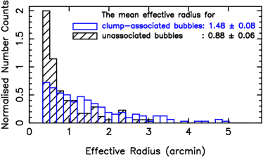
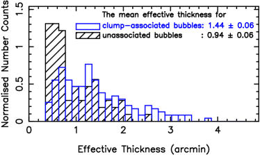
Figure 11: Distributions of the effective radius (upper panel) and the effective thickness (lower panel) for the MWP bubbles with and without associated molecular clumps.

As shown in Fig. 9, the probability of finding GRS molecular clumps within two effective bubble radii is significantly higher than in the outer regions. Hence, we define a “clump-associated bubble” as a bubble that has associated molecular clump(s) within two effective bubble radii and the velocity difference between the bubble and the clump(s) is less than $\delta V=7$ km s^-1. 184 ($\sim$ 60%) out of the 309 MWP bubbles meet the criteria and 117 bubbles ($\sim$ 38%) have more than one matched clump. We define the bubbles which have no associated clumps within three effective bubble radii as “clump-unassociated”. This group contains 101 ($\sim$ 33%) MWP bubbles. The clumps located between two and three effective bubble radii are less significantly correlated with the bubbles and these cases cannot be clearly classified and are not included in the analysis. In the following, we discuss the properties of the physical sizes and the central ionizing sources of the clump-associated and clump-unassociated bubbles.

The distributions of the effective radius and thickness of the clump-associated and unassociated bubbles are compared (see Fig. 11) and listed in Table 1. Clearly, the clump-associated bubbles tend to be larger and thicker in physical sizes, and the differences are always significant, e.g. the probability that the clump-associated and clump-unassociated bubbles are drawn from populations with the same mean physical effective radius is only 2.0%. This contradicts with the result revealed by the MYSOs around 322 CH06&07 bubbles (Thompson et al., 2012). Thompson et al. (2012) found the MYSO-associated bubbles tend to be smaller and thinner than the MYSO-unassociated bubbles. We attribute this discrepancy to the incompleteness of the CH06&07 catalogue. Churchwell et al. (2006) suggested that the incompleteness of the CH06&07 bubble catalogue is $\sim$ 50%. The recently released bubble catalogue (Simpson et al., 2012) that we used in this work has ten times more bubbles than in the CH06&07 catalogue.

For a further inspection of this contradiction, we cross match the 309 MWP bubbles with the MYSO sample of Urquhart et al. (2008). According to Kendrew et al. (2012), if the angular separation between a MYSO and a bubble is less than 1.6 effective bubble radii, they are taken as coincidence. 102 ($\sim$ 33%) of the 309 MWP bubbles are then found to be MYSO-associated. The bubbles that have no MYSOs within two effective bubble radii are taken as MYSO-unassociated(Kendrew et al., 2012). 195 ($\sim$ 63%) of the 309 MWP bubbles are selected. The mean values for the effective radius and thickness are then calculated and compared in Table 1. With the more complete bubble sample, and the same MYSO sample with Thompson et al. (2012), we claim that both of the MYSO-associated and the clump-associated bubbles have larger effective radius and thickness than the un-associated ones.

Dale et al. (2009) suggested that the bubbles with smaller radii and thinner shells should be younger than the larger and thicker ones. Hence, the mean values of the effective bubble radii and thickness could be rough indicators of the bubble ages. From Table 1, we do see such differences between the clump-/MYSO-associated and the clump-/MYSO-unassociated bubbles in their mean physical effective radii and thicknesses. Therefore we speculate that the age of bubbles might be a factor for a bubble to have associated molecular clumps or MYSOs.

In addition, we also try to search for the differences of their central ionizing source(s). We calculated the ionizing photon rate (Matsakis et al., 1976):

$$N_{Ly}~{}=~{}7.5~{}\times~{}10^{46}~{}F_{\nu}~{}\nu^{0.1}~{}d^{2}~{}T_{e}^{-0.45}~{}[photos~{}s^{-1}]$$ (3)

where $F_{\nu}$ is the flux density in Jy, derived from the MAGPIS survey (Helfand et al., 2006), $\nu$ is the observed frequency in GHz, $d$ is the bubble distance to the Sun in kpc, which should be consistent with the distance of central ionizing source(s), and $T_{e}$ is the electron temperature in 10⁴ K. Here, we adopted the typical electron temperature 8500 K for the H II regions. Different values are found for the mean ionizing photon rate log($N_{Ly}$): 47.54 $\pm$ 0.09 for the clump-associate bubbles and 47.01 $\pm$ 0.13 for the bubbles without clumps. The probability that the two results are taken from the populations with the same mean ionizing photon rate is less than 0.1%. Hence, the luminosity of central ionizing source(s) seems to be another factor for a bubble to have associated molecular clumps.

The reaction of molecular gas to the expansion of H II regions is complex and determined by several factors: the luminosity of central ionizing source(s), the ability of central ionizing source(s) to ionize the surrounding gas, which depends on the ambient gas density and the strength of accretion, and the ability of H II region to drive out the ambient neutral gas, which depends on the escape velocity of the whole system with respect to the sound speed of the ionized gas (see Dale et al., 2012b, for detail). As shown above, both the age of the interstellar bubbles and the luminosity of the central ionizing source(s) seem to have certain impacts on a bubble to have associated molecular clump(s)/ MYSO(s). Additionally, the properties of the ambient gaseous environment, e.g. the density field and the velocity field, which might also play an important role, deserves more attention in the future high-resolution observations.

4.2 The properties of bubble-associated and bubble-unassociated molecular clumps

In this part, we simply switch our targets from the MWP interstellar bubbles to the GRS molecular clumps. We compare the properties of “bubble-associated” and “bubble-unassociated” clumps. With the same velecity selection criteria. 492 out of the 5 106 GRS clumps are found to be associated with the 309 interstellar bubbles. For all of the clumps which are located outside the three effective radii from any of the MWP bubbles, we define them as the bubble-unassociated clumps.

We find that the mean velocity FWHM extent (V_FWHM, defined as 2.35 times the velocity dispersion of the molecular clump, given by Rathborne et al., 2009) is 1.71 $\pm$ 0.04 km s^-1 for the bubble-associated clumps, and 1.25 $\pm$ 0.01 km s^-1 for the bubble-unassociated clumps. The peak main beam temperature (T${}_{MB~{}peak}$) for the two groups are 7.33 $\pm$ 0.13 K and 4.68 $\pm$ 0.03 K, respectively (see Fig. 12). It is clear that the bubble-associated molecular clumps tend to have larger T${}_{MB~{}peak}$ and V_FWHM, and have larger peak intensity and larger peak H₂ column density consequently, namely, they are brighter and denser. Dale et al. (2007) examined the impact of the external ionizing irradiation on a turbulent molecular cloud numerically. They found that the molecular cloud exposed to the ionizing radiation field tends to be denser, and forms about twice as many young stars in comparison to the control model. A natural explanation is that the shock driven by the ionizing feedback will sweep up and compress the surrounding neutral gas, hence, the molecular clumps influenced by the feedback tend to be brighter and denser. The differences between the bubble-associated and bubble-unassociated molecular clumps might reflect the influence of ionizing feedback from central massive star(s)/star cluster that creates the bubbles.

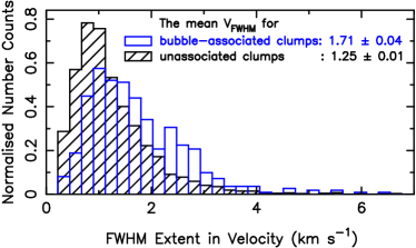
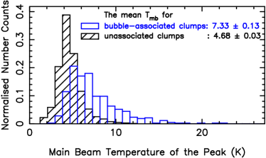
Figure 12: Distributions of the FWHM extent in velocity (upper panel) and the main beam temperature of the peak (lower panel) for the bubble-associated and unassociated molecular clumps.

4.3 Triggered material accumulation and star formation by the expansion of bubbles?

The observational over density of molecular gas near the bubble rims is consistent with the scenario that the bubble expansion has a prominent impact on the ambient gas and triggers the material accumulation (see Deharveng et al., 2010). But it can also be interpreted as a fact that the bubbles tend to form in the high density regions of molecular gas.

Table 2: Properties for the MYSO-associated and unassociated bubble-clump complexes.

		MYSO-	MYSO-	T-statistic
		associated	unassociated	significance
mean effective radius
	apparent (arcmin)	1.65 $\pm$ 0.15	1.33 $\pm$ 0.08	4.3%
	physical (pc)	3.45 $\pm$ 0.40	2.53 $\pm$ 0.16	1.8%
mean effective thickness
	apparent (arcmin)	1.54 $\pm$ 0.12	1.33 $\pm$ 0.06	8.6%
	physical (pc)	3.23 $\pm$ 0.35	2.52 $\pm$ 0.14	3.7%
ionizing photo rate
	log($N_{Ly}$)	47.64 $\pm$ 0.14	47.44 $\pm$ 0.12	26.7%
FWHM extent in velocity
	(km s-1)	1.81 $\pm$ 0.06	1.66 $\pm$ 0.06	7.8%
main beam temperature of the peak
	(K)	7.58 $\pm$ 0.18	7.27 $\pm$ 0.17	22.0%

If the later is correct, one question would be that why the distribution of the molecular gas peculiarly peaks near the bubble rims. The bubble rims are traced by the 8 $\mu$m emission, which is dominanted by the emission from the PAH or clusters of molecules. These species are excited by the absorption of far-UV photons leaking from the central ionizing sources and trace the expanding ionization fronts of H II regions. Hence, the bubble rim is time-dependent, increasing with time. If the bubbles formed in high density regions of neutral gas, for the spherical or ring-like (Beaumont & Williams, 2010) morphology of the bubbles, the column density of molecular gas in the outer regions of the bubbles is expected to be close to that near the bubble rims, because of the similar integrated path length penetrating the line of sight. However, this is not the case as we found in Fig. 7, that the material density falls rapidly from the angular distance from one effective bubble radius to larger distances.

Alternatively, the influence of bubble expansion on the ambient gas can naturally explain the observed properties of gas distribution. The expansion of bubbles is caused by the higher pressure in the ionized gas than its surrounding neutral material. This process is accompanied by the accumulation of neutral material between the ionizing front and the shock front (e.g. see Deharveng et al., 2010). Our results suggest that some of the bubble-associated clumps are probably triggered by the collecting process during the bubble expansion.

More intriguing questions are whether the bubble-associated molecular clumps are able to generate new stars, and whether the bubble expansion influences the formation of the new stars. In our sample, as we mentioned above, 184 bubbles have associated molecular clump(s). They are now named as “bubble-clump complexes”. We check their associations with MYSOs.

If the bubble expansion does not influence the star formation in the ambient dense gas, one would expect no differences between the properties of the MYSO-associated bubble-clump complexes and the MYSO-unassociated complexes. However, we found differences in the mean effective radius and the thickness for the bubbles in different groups as given in Table 2. Those differences are around 3$\sigma$ for the physical sizes, and slightly above 2$\sigma$ for the apparent sizes. The bubbles in the MYSO-associated complex are larger and thicker, hence, tend to be older. We further evaluate other factors which may take effect in this process for the two different groups, such as the mean ionizing photon rate log$N_{Ly}$ of the central ionizing source(s), the peak main beam temperature and the FWHM extent in velocity for the clumps, but no significant differences were found. Therefore we speculate that, as the bubble in the complex evolves, the relatively younger MYSO-unassociated complexes could breed MYSOs, and may finally turn to be MYSO-associated. If so, the MYSO-unassociated complexes are the potential sites of triggering SF by the feedback of H II regions. To verify this hypothesis, detailed studies on the physical conditions and dynamical properties of the neutral gas are necessary. High-resolution observations of different molecular species, e.g. ¹³CO, NH₃, CH₃OH, are required.

4.4 The fraction of molecular clumps associated with MWP bubbles.

As discussed in section 4.2, a bubble-associated clump is defined as a clump that has one bubble within two effective bubble radii. To solve the projection effect, their velocity difference should be less than $\delta V=7$ km s^-1. 492 (about 8%) of the 6 124 molecular clumps are selected finally. This percentage is the lower limit, because only 309 of the 1 637 MWP bubbles in the sky coverage of the GRS have their line-of-sight velocities measured. If no constraint was made on the velocity difference, namely, the projection effect was not considered, this number increases to 788 (about 13%), that match the 309 interstellar bubbles. This leads to a significant percentage (about 38%) of false identification.

To estimate the fraction of molecular clumps associated with MWP bubbles, we used all the 1 637 MWP bubbles falling into the sky coverage of the GRS and made no constraints on the velocity difference. 1 980 (about 32%) of the 6 124 molecular clumps are then selected out to have matched MWP bubbles. By assuming that 38% of them are mistaken due to the projection effect, the number of associations is reduced to 1 236 (about 20%). This fraction varies from 16% to 22% corresponding to $\delta V=5$ $-$ 9 km s^-1.

The result seems to be consistent with the previous estimates of the fraction of MYSOs associated with the interstellar bubbles. By analyzing the associations of RMS MYSOs and the CH06&07 bubbles, Thompson et al. (2012) estimated the fraction of MYSOs triggered by the expansion of bubbles is between 14% and 30%. By using a more complete catalogue of bubbles, Kendrew et al. (2012) obtained a fraction of $\sim$ 22% $\pm$ 2%. With a relative small sample of bubbles, this fraction was estimated to be 18% and 20% by Deharveng et al. (2010) and Watson et al. (2010), respectively. Note however, that the projection effect was not considered in any of the estimates mentioned above. Their results might be somehow overestimated.

5 Conclusions

We made a statistical study of the gaseous environment of the interstellar bubbles identified by the Milky Way Project (Simpson et al., 2012). Our conclusions are summarized below:

$\bullet$ By making cross-identification between the MWP Spitzer interstellar bubbles and the Galactic H II region catalogue compiled by us, we obtain the velocity information for 818 MWP bubbles. As a result, 721 bubbles have determined distances, either photometric, trigonometric or kinematic, which is nearly four times larger than previous known.

$\bullet$ We used three methods to study the gaseous environment of MWP bubbles:

(1) The mean azimuthally averaged radial profile of ¹³CO emission, with which we found clear emission excesses at the angular distances less than three effective bubble radii. A significant peak appears close to one effective bubble radius, corresponding to the bubble rims. At larger angular distances, the mean profile gradually falls and finally reaches the values close to the background level.

(2) The surface number density of molecular clumps is also found to be enhanced toward the bubble rims. The excess at smaller angular distances is more prominent than that shown by the mean azimuthally averaged radial profile of ¹³CO emission. A significant peak at a 7.7 $\sigma$ level is found near one effective bubble radius. The surface number density falls more sharply at larger angular distances.

(3) The cross-correlation function of the MWP bubbles and the GRS molecular clumps gives consistent results with that of the surface number density of molecular clumps. The affection of intrinsic clustering of the GRS clumps is estimated and found to be negligible. At larger angular distances, e.g. $>$ three effective bubble radii, the molecular clumps are essentially not correlated with the interstellar bubbles.

Our results for the distribution of gas component around the bubbles are consistent with the analysis based on the associations between the MYSOs and the bubbles. The significant peak near the bubble rims and the variations of molecular gas along the angular distance make us to speculate that some of the bubble-associated clumps might be triggered by the expansion of bubbles.

$\bullet$ About 60% of the investigated interstellar bubbles have associated molecular clumps. By comparing the effective radius, thickness and the ionizing source(s) of the clump-associated and clump-unassociated bubbles, we speculate that the age and the luminosity of central ionizing source(s) have certain impacts for a bubble to have associated molecular clumps.

$\bullet$ For the bubble-clump complexes, we inspected their associations with MYSOs. The bubbles in the MYSO-associated complex are found to be larger and thicker, hence relative older. This implies an evolutionary sequence that the relative younger MYSO-unassociated bubble-clump complexes might breed MYSOs, and evolve to the phase of MYSO-associated.

$\bullet$ The fraction of molecular clumps associated with the MWP bubbles is estimated to be about 20% after considering the projection effect.

Appendix A Spitzer interstellar bubbles with velocity information

We cross-identified the MWP bubbles and the Galactic H II regions, 818 matched pairs are found and listed in Table A, which is available in its entirety in the online material, and a portion is presented below for guidance regarding its form and content.

[x]lccrrrlrrrrrrlr Matched pairs of MWP bubbles and Galactic H II regions. Columns 1 to 4 list the MWP name, Galactic longitude, Galactic latitude, and effective radius for each bubble; Cols 5 and 6 give the Galactic longitude and Galactic latitude of the associated HII regions, taken from the reference listed in Col. 7; Col. 8 is the line-of-sight velocity for each HII region; Cols. 9 to 10 list the trigonometric or photometric distance and the uncertainty when available from the reference shown in Col. 11; Col. 12 gives the kinematic distance estimated with a flat rotation curve with R₀ = 8.3 kpc and $\theta_{0}$ = 239 km s^-1; Col. 13 is the uncertainty of the kinematic distance estimated by considering a velocity uncertainty of $\pm$ 7 km s^-1; Col. 14 gives the solution of the kinematic distance ambiguity: kfar - the farther kinematic distance is adopted; ktan - the source is located at the tangential point; knear - the nearer kinematic distance is adopted; 3kpcn/3kpcf - the source is in the near or far 3-kpc arm (see e.g., Dame & Thaddeus 2011); and Col. 15 is the reference.
References: abbr11: Anderson et al. (2011); abbr12: Anderson et al. (2012); ab09: Anderson & Bania (2009); ahck02: Araya et al. (2002); bwl09: Beuther et al. (2009); brba11: Balser et al. (2011); brm+09: Brunthaler et al. (2009); bab12: Bania et al. (2012); bfs82: Blitz et al. (1982); bdc01: Blum et al. (2001); bnt89: Bronfman et al. (1989); brof96: Bronfman et al. (1996); ch87: Caswell & Haynes (1987); cwc90: Churchwell et al. (1990); dwbw80: Downes et al. (1980); frwc03: Fish et al. (2003); gcbt88: Grabelsky et al. (1988); gg76: Georgelin & Georgelin (1976); gm11: Green & McClure-Griffiths (2011); hze+11: Han et al. (2011); jd12: Jones & Dickey (2012); kb94: Kuchar & Bania (1994); kjb+03: Kolpak et al. (2003); lra+11: Lépine et al. (2011); lock79: Lockman (1979); lock89: Lockman (1989); lock96: Lockman et al. (1996); msh+11: Motogi et al. (2011); mdf+11: Moisés et al. (2011); noh+11: Nagayama et al. (2011); pdd04: Paladini et al. (2004); pco10: Pinheiro et al. (2010); rjh+09: Roman-Duval et al. (2009); rus03: Russeil (2003); rza+12: Russeil et al. (2012); srm+09: Sanna et al. (2009); sh10: Stead & Hoare (2010); st79: Silverglate & Terzian (1979); srby87: Solomon et al. (1987); srbm10: Sato et al. (2010b); swa+04: Sewilo et al. (2004); uhl12: Urquhart et al. (2012); was+03: Watson et al. (2003); wam82: Wink et al. (1982); wwb83: Wink et al. (1983); wmgm70: Wilson et al. (1970); xmr+11: Xu et al. (2011).
MWP name l_bubble b_bubble Reff l${}_{\rm H\,II}$ b${}_{\rm H\,II}$ Ref. v${}_{\rm H\,II}$ d_o d_erro Ref. d_k d_k-erro Mark Ref.
$(^{\circ})$ $(^{\circ})$ (^′) $(^{\circ})$ $(^{\circ})$ (km/s) (kpc) (kpc) (kpc) (kpc)
(1) (2) (3) (4) (5) (6) (7) (8) (9) (10) (11) (12) (13) (14) (15)
continued.
MWP name l_bubble b_bubble Reff l${}_{\rm H\,II}$ b${}_{\rm H\,II}$ Ref. v${}_{\rm H\,II}$ d_o d_erro Ref. d_k d_k-erro Mark Ref.
$(^{\circ})$ $(^{\circ})$ (^′) $(^{\circ})$ $(^{\circ})$ (km/s) (kpc) (kpc) (kpc) (kpc)
(1) (2) (3) (4) (5) (6) (7) (8) (9) (10) (11) (12) (13) (14) (15)
MWP1G000127+000485 0.127 +0.048 3.58 0.09 0.01 wwb83 $-$29.70
MWP1G000140$-$001173 0.140 $-$0.117 3.62 0.094 $-$0.154 brof96 16.00
MWP1G000280$-$004800S 0.28 $-$0.48 0.59 0.284 $-$0.478 dwbw80 19.25 7.86 0.16 knear rus03
MWP1G000515$-$007049 0.515 $-$0.705 3.24 0.489 $-$0.668 dwbw80 17.50 7.46 0.33 knear rus03
MWP1G000530+001800S 0.53 +0.18 0.50 0.527 0.182 brof96 $-$3.05

References

- Anderson & Bania (2009) Anderson, L. D. & Bania, T. M. 2009, ApJ, 690, 706
- Anderson et al. (2011) Anderson, L. D., Bania, T. M., Balser, D. S., & Rood, R. T. 2011, ApJS, 194, 32
- Anderson et al. (2012) Anderson, L. D., Bania, T. M., Balser, D. S., & Rood, R. T. 2012, ApJ, 754, 62
- Araya et al. (2002) Araya, E., Hofner, P., Churchwell, E., & Kurtz, S. 2002, ApJS, 138, 63
- Balser et al. (2011) Balser, D. S., Rood, R. T., Bania, T. M., & Anderson, L. D. 2011, ApJ, 738, 27
- Bania et al. (2012) Bania, T. M., Anderson, L. D., & Balser, D. S. 2012, ApJ, 759, 96
- Beaumont & Williams (2010) Beaumont, C. N. & Williams, J. P. 2010, ApJ, 709, 791
- Benjamin et al. (2003) Benjamin, R. A., Churchwell, E., Babler, B. L., et al. 2003, PASP, 115, 953
- Beuther et al. (2009) Beuther, H., Walsh, A. J., & Longmore, S. N. 2009, ApJS, 184, 366
- Bik et al. (2010) Bik, A., Puga, E., Waters, L. B. F. M., et al. 2010, ApJ, 713, 883
- Blitz et al. (1982) Blitz, L., Fich, M., & Stark, A. A. 1982, ApJS, 49, 183
- Blum et al. (2001) Blum, R. D., Damineli, A., & Conti, P. S. 2001, AJ, 121, 3149
- Bradshaw et al. (2011) Bradshaw, E. J., Almaini, O., Hartley, W. G., et al. 2011, MNRAS, 415, 2626
- Bronfman et al. (1989) Bronfman, L., Nyman, L., & Thaddeus, P. 1989, in Lecture Notes in Physics, Berlin Springer Verlag, Vol. 331, The Physics and Chemistry of Interstellar Molecular Clouds - mm and Sub-mm Observations in Astrophysics, ed. G. Winnewisser & J. T. Armstrong, 139–140
- Bronfman et al. (1996) Bronfman, L., Nyman, L.-A., & May, J. 1996, A&AS, 115, 81
- Brunthaler et al. (2009) Brunthaler, A., Reid, M. J., Menten, K. M., et al. 2009, ApJ, 693, 424
- Brunthaler et al. (2011) Brunthaler, A., Reid, M. J., Menten, K. M., et al. 2011, Astronomische Nachrichten, 332, 461
- Carey et al. (2009) Carey, S. J., Noriega-Crespo, A., Mizuno, D. R., et al. 2009, PASP, 121, 76
- Caswell & Haynes (1987) Caswell, J. L. & Haynes, R. F. 1987, A&A, 171, 261
- Churchwell et al. (1990) Churchwell, E., Walmsley, C. M., & Cesaroni, R. 1990, A&AS, 83, 119
- Churchwell et al. (2006) Churchwell, E., Povich, M. S., Allen, D., et al. 2006, ApJ, 649, 759
- Churchwell et al. (2007) Churchwell, E., Watson, D. F., Povich, M. S., et al. 2007, ApJ, 670, 428
- Dale et al. (2012a) Dale, J. E., Ercolano, B., & Bonnell, I. A. 2012a, MNRAS, 427, 2852
- Dale et al. (2012b) Dale, J. E., Ercolano, B., & Bonnell, I. A. 2012b, MNRAS, 424, 377
- Dale et al. (2009) Dale, J. E., Wünsch, R., Whitworth, A., & Palouš, J. 2009, MNRAS, 398, 1537
- Dale et al. (2007) Dale, J. E., Clark, P. C., & Bonnell, I. A. 2007, MNRAS, 377, 535
- Dame et al. (2001) Dame, T. M., Hartmann, D., & Thaddeus, P. 2001, ApJ, 547, 792
- Dame & Thaddeus (2011) Dame, T. M. & Thaddeus, P. 2011, ApJL, 734, L24
- Deharveng et al. (2010) Deharveng, L., Schuller, F., Anderson, L. D., et al. 2010, A&A, 523, A6
- Deharveng et al. (2005) Deharveng, L., Zavagno, A., & Caplan, J. 2005, A&A, 433, 565
- Deharveng et al. (2009) Deharveng, L., Zavagno, A., Schuller, F., et al. 2009, A&A, 496, 177
- Dewangan & Ojha (2012) Dewangan, L. K. & Ojha, D. K. 2012, MNRAS, 371
- Dirienzo et al. (2012) Dirienzo, W. J., Indebetouw, R., Brogan, C., et al. 2012, AJ, 144, 173
- Downes et al. (1980) Downes, D., Wilson, T. L., Bieging, J., & Wink, J. 1980, A&AS, 40, 379
- Elmegreen et al. (1995) Elmegreen, B. G., Kimura, T., & Tosa, M. 1995, ApJ, 451, 675
- Elmegreen & Lada (1977) Elmegreen, B. G. & Lada, C. J. 1977, ApJ, 214, 725
- Fish et al. (2003) Fish, V. L., Reid, M. J., Wilner, D. J., & Churchwell, E. 2003, ApJ, 587, 701
- Garcia-Segura & Franco (1996) Garcia-Segura, G. & Franco, J. 1996, ApJ, 469, 171
- Georgelin & Georgelin (1976) Georgelin, Y. M. & Georgelin, Y. P. 1976, A&A, 49, 57
- Grabelsky et al. (1988) Grabelsky, D. A., Cohen, R. S., Bronfman, L., & Thaddeus, P. 1988, ApJ, 331, 181
- Green & McClure-Griffiths (2011) Green, J. A., & McClure-Griffiths, N. M. 2011, MNRAS, 417, 2500
- Helfand et al. (2006) Helfand, D. J., Becker, R. H., White, R. L., Fallon, A., & Tuttle, S. 2006, AJ, 131, 2525
- Heyer et al. (1998) Heyer, M. H., Brunt, C., Snell, R. L., et al. 1998, ApJS, 115, 241
- Hou et al. (2009) Hou, L. G., Han, J. L., & Shi, W. B. 2009, A&A, 499, 473
- Hou & Han (2013) Hou, L. G., & Han, J. L. 2013, IAU Symposium, 292, 106
- Han et al. (2011) Han, X.-H., Zhou, J.-J., Esimbek, J., Wu, G., & Gao, M.-F. 2011, Research in Astronomy and Astrophysics, 11, 156
- Jackson et al. (2006) Jackson, J. M., Rathborne, J. M., Shah, R. Y., et al. 2006, ApJS, 163, 145
- Ji et al. (2012) Ji, W.-G., Zhou, J.-J., Esimbek, J., et al. 2012, A&A, 544, A39
- Jones & Dickey (2012) Jones, C. & Dickey, J. M. 2012, ApJ, 753, 62
- Kang et al. (2009) Kang, M., Bieging, J. H., Kulesa, C. A., & Lee, Y. 2009, ApJ, 701, 454
- Kendrew et al. (2012) Kendrew, S., Simpson, R., Bressert, E., et al. 2012, ApJ, 755, 71
- Kolpak et al. (2003) Kolpak, M. A., Jackson, J. M., Bania, T. M., Clemens, D. P., & Dickey, J. M. 2003, ApJ, 582, 756
- Kuchar & Bania (1994) Kuchar, T. A., & Bania, T. M. 1994, ApJ, 436, 117
- Landy & Szalay (1993) Landy, S. D. & Szalay, A. S. 1993, ApJ, 412, 64
- Lee et al. (2001) Lee, Y., Stark, A. A., Kim, H.-G., & Moon, D.-S. 2001, ApJS, 136, 137
- Lefloch & Lazareff (1994) Lefloch, B. & Lazareff, B. 1994, A&A, 289, 559
- Lépine et al. (2011) Lépine, J. R. D., Roman-Lopes, A., Abraham, Z., Junqueira, T. C., & Mishurov, Y. N. 2011, MNRAS, 414, 1607
- Li et al. (2013) Li, J.-Y., Jiang, Z.-B., Liu, Y., & Wang, Y. 2013, Research in Astronomy and Astrophysics, 13, 921
- Lockman (1979) Lockman, F. J. 1979, ApJ, 232, 761
- Lockman (1989) Lockman, F. J. 1989, ApJS, 71, 469
- Lockman et al. (1996) Lockman, F. J., Pisano, D. J., & Howard, G. J. 1996, ApJ, 472, 173
- Martins et al. (2010) Martins, F., Pomarès, M., Deharveng, L., Zavagno, A., & Bouret, J. C. 2010, A&A, 510, A32
- Matzner (2002) Matzner, C. D. 2002, ApJ, 566, 302
- Matsakis et al. (1976) Matsakis, D. N., Evans, II, N. J., Sato, T., & Zuckerman, B. 1976, AJ, 81, 172
- Mizuno & Fukui (2004) Mizuno, A. & Fukui, Y. 2004, in Astronomical Society of the Pacific Conference Series, Vol. 317, Milky Way Surveys: The Structure and Evolution of our Galaxy, ed. D. Clemens, R. Shah, & T. Brainerd, 59
- Mizuno et al. (2010) Mizuno, D. R., Kraemer, K. E., Flagey, N., et al. 2010, AJ, 139, 1542
- Moisés et al. (2011) Moisés, A. P., Damineli, A., Figuerêdo, E., et al. 2011, MNRAS, 411, 705
- Motogi et al. (2011) Motogi, K., Sorai, K., Habe, A., et al. 2011, PASJ, 63, 31
- Nagayama et al. (2011) Nagayama, T., Omodaka, T., Handa, T., et al. 2011, PASJ, 63, 719
- Paladini et al. (2004) Paladini, R., Davies, R. D., & DeZotti, G. 2004, MNRAS, 347, 237
- Paron et al. (2009) Paron, S., Cichowolski, S., & Ortega, M. E. 2009, A&A, 506, 789
- Petriella et al. (2010) Petriella, A., Paron, S., & Giacani, E. 2010, A&A, 513, A44
- Pinheiro et al. (2010) Pinheiro, M. C., Copetti, M. V. F., & Oliveira, V. A. 2010, A&A, 521, A26
- Povich et al. (2009) Povich, M. S., Churchwell, E., Bieging, J. H., et al. 2009, ApJ, 696, 1278
- Puga et al. (2009) Puga, E., Hony, S., Neiner, C., et al. 2009, A&A, 503, 107
- Rathborne et al. (2009) Rathborne, J. M., Johnson, A. M., Jackson, J. M., Shah, R. Y., & Simon, R. 2009, ApJS, 182, 131
- Roman-Duval et al. (2009) Roman-Duval, J., Jackson, J. M., Heyer, M., et al. 2009, ApJ, 699, 1153
- Russeil (2003) Russeil, D. 2003, A&A, 397, 133
- Russeil et al. (2012) Russeil, D., Zavagno, A., Adami, C., et al. 2012, A&A, 538, A142
- Samal et al. (2012) Samal, M. R., Pandey, A. K., Ojha, D. K., et al. 2012, ApJ, 755, 20
- Sanna et al. (2009) Sanna, A., Reid, M. J., Moscadelli, L., et al. 2009, ApJ, 706, 464
- Sanders et al. (1986) Sanders, D. B., Clemens, D. P., Scoville, N. Z., & Solomon, P. M. 1986, ApJS, 60, 1
- Schönrich et al. (2010) Schönrich, R., Binney, J., & Dehnen, W. 2010, MNRAS, 403, 1829
- Sherman (2012) Sherman, R. A. 2012, ApJ, 760, 58
- Silverglate & Terzian (1979) Silverglate, P. R., & Terzian, Y. 1979, ApJS, 39, 157
- Simpson et al. (2012) Simpson, R. J., Povich, M. S., Kendrew, S., et al. 2012, MNRAS, 424, 2442
- Solomon et al. (1987) Solomon, P. M., Rivolo, A. R., Barrett, J., & Yahil, A. 1987, ApJ, 319, 730
- Sato et al. (2010b) Sato, M., Reid, M. J., Brunthaler, A., & Menten, K. M. 2010b, ApJ, 720, 1055
- Stead & Hoare (2010) Stead, J. J. & Hoare, M. G. 2010, MNRAS, 407, 923
- Sewilo et al. (2004) Sewilo, M., Watson, C., Araya, E., et al. 2004, ApJS, 154, 553
- Thompson et al. (2012) Thompson, M. A., Urquhart, J. S., Moore, T. J. T., & Morgan, L. K. 2012, MNRAS, 421, 408
- Urquhart et al. (2008) Urquhart, J. S., Hoare, M. G., Lumsden, S. L., Oudmaijer, R. D., & Moore, T. J. T. 2008, in Astronomical Society of the Pacific Conference Series, Vol. 387, Massive Star Formation: Observations Confront Theory, ed. H. Beuther, H. Linz, & T. Henning, 381
- Urquhart et al. (2012) Urquhart, J. S., Hoare, M. G., Lumsden, S. L., et al. 2012, MNRAS, 420, 1656
- Watson et al. (2003) Watson, C., Araya, E., Sewilo, M., et al. 2003, ApJ, 587, 714
- Watson et al. (2010) Watson, C., Hanspal, U., & Mengistu, A. 2010, ApJ, 716, 1478
- Watson et al. (2008) Watson, C., Povich, M. S., Churchwell, E. B., et al. 2008, ApJ, 681, 1341
- Wilson et al. (1970) Wilson, T. L., Mezger, P. G., Gardner, F. F., & Milne, D. K. 1970, A&A, 6, 364
- Wink et al. (1982) Wink, J. E., Altenhoff, W. J., & Mezger, P. G. 1982, A&A, 108, 227
- Wink et al. (1983) Wink, J. E., Wilson, T. L., & Bieging, J. H. 1983, A&A, 127, 211
- Xu et al. (2011) Xu, Y., Moscadelli, L., Reid, M. J., et al. 2011, ApJ, 733, 25
- Zavagno et al. (2010) Zavagno, A., Anderson, L. D., Russeil, D., et al. 2010, A&A, 518, L101
- Zhang & Wang (2012a) Zhang, C. P. & Wang, J. J. 2012a, A&A, 544, A11
- Zhang & Wang (2013) Zhang, C.-P., & Wang, J.-J. 2013, Research in Astronomy and Astrophysics, 13, 47
- Zhang et al. (2013) Zhang, C.-P., Wang, J.-J., & Xu, J.-L. 2013, A&A, 550, A117