Multitask Diffusion Adaptation over Networks

Abstract

Adaptive networks are suitable for decentralized inference tasks, e.g., to monitor complex natural phenomena. Recent research works have intensively studied distributed optimization problems in the case where the nodes have to estimate a single optimum parameter vector collaboratively. However, there are many important applications that are multitask-oriented in the sense that there are multiple optimum parameter vectors to be inferred simultaneously, in a collaborative manner, over the area covered by the network. In this paper, we employ diffusion strategies to develop distributed algorithms that address multitask problems by minimizing an appropriate mean-square error criterion with $\ell_{2}$-regularization. The stability and convergence of the algorithm in the mean and in the mean-square sense is analyzed. Simulations are conducted to verify the theoretical findings, and to illustrate how the distributed strategy can be used in several useful applications related to spectral sensing, target localization, and hyperspectral data unmixing.

EDICS: NET-ADEG, NET-DISP, MLR-DIST, SSP-PERF

I Introduction

Distributed adaptation over networks has emerged as an attractive and challenging research area with the advent of multi-agent (wireless or wireline) networks. Accessible overviews of recent results in the field can be found in [Sayed2013diff, Sayed2013intr]. In adaptive networks, the interconnected nodes have to continually learn and adapt, as well as perform preassigned tasks such as parameter estimation from observations collected by the dispersed agents. Although centralized strategies with a fusion center can benefit more fully from information collected throughout the network but stored at a single point, in most cases, distributed strategies are more attractive to solve inference problems in a collaborative and autonomous manner. Scalability, robustness, and low-power consumption are key characteristics of these strategies. Applications include environment monitoring, but also modeling of self-organized behavior observed in nature such as bird flight in formation and fish schooling [Sayed2013diff, Tu2011Mobile].

There are several useful distributed strategies for sequential data processing over networks including consensus strategies [Tsitsiklis1984, Xiao2004, Braca2008, Nedic2009, Kar2009, Srivastava2011], incremental strategies [Bertsekas1997, Nedic2001, Rabbat2005, Blatt2007, Lopes2007incr], and diffusion strategies [Sayed2013diff, Sayed2013intr, Lopes2008diff, Cattivelli2010diff, ChenUCLA2012, ChenUCLA2013]. Incremental techniques require the determination of a cyclic path that runs across the nodes, which is generally a challenging (NP-hard) task to perform. Besides, incremental solutions can be problematic for adaptation over networks because they are sensitive to link failures. On the other hand, diffusion strategies are attractive since they are scalable, robust, and enable continuous adaptation and learning. In addition, for data processing over adaptive networks, diffusion strategies have been shown to have superior stability and performance ranges [Tu2012] than consensus-based implementations. Consequently, we shall focus on diffusion-type implementations in the sequel. The diffusion LMS strategy was proposed and studied in [Lopes2008diff, Cattivelli2010diff]. Its performance in the presence of imperfect information exchange and model non-stationarity was analyzed in [Tu2011, Khalili2012, Zhao2012impe]. Diffusion LMS with $\ell_{1}$-norm regularization was considered in [Lorenzo2012, Liu2012, Chouvardas2012, Lorenzo2013spar] to promote sparsity in the model. In [Chouvardas2011set], the problem of distributed learning in diffusion networks was addressed by deriving projection algorithms onto convex sets. Diffusion RLS over adaptive networks was studied in [Cattivelli2008, Bertrand2011RLS]. More recently, a distributed dictionary learning algorithm based on a diffusion strategy was derived in [chainais2013distributed, chainais2013learning, Wee2013]. This literature mainly considers quadratic cost functions and linear models where systems are characterized by a parameter vector in the Euclidean space. Extensions to more general cost functions that are not necessarily quadratic and to more general data models are studied in [ChenUCLA2012, ChenUCLA2013] in the context of adaptation and learning over networks. Moreover, several other works explored distributed estimation for nonlinear input-output relationships defined in a functional space, such as reproducing kernel Hilbert spaces. For instance, in [Predd2006WSN], inference is performed with a regularized kernel least-squares estimator, where the distributed information-sharing strategy consisted of successive orthogonal projections. Distributed estimation based on adaptive kernel regression [richard2009online, honeine2007line] is also studied in [Honeine2010WSN, honeine2009functional, honeine2008regression, honeine2008distributed], with information passed from node to node in an incremental manner. In [Chen2010WSN], non-negative distributed regression is considered for nonlinear model inference subject to non-negativity constraints, where the diffusion strategy is used to conduct information exchange.

An inspection of the existing literature on distributed algorithms shows that most works focus primarily, though not exclusively [Tu2012Asilomar, Zhao2012, Bogdanovic2013], on the case where the nodes have to estimate a single optimum parameter vector collaboratively. We shall refer to problems of this type as single-task problems. However, many problems of interest happen to be multitask-oriented in the sense that there are multiple optimum parameter vectors to be inferred simultaneously and in a collaborative manner. The multitask learning problem is relevant in several machine learning formulations and has been studied in the machine learning community in several contexts. For example, the problem finds applications in web page categorization [chen2009mtl], web-search ranking [Chapelle2011mtl], and disease progression modeling [zhou2011mtl], among other areas. Clearly, this concept is also relevant in the context of distributed estimation and adaptation over networks. Initial investigations along these lines for the traditional diffusion strategy appear in [Zhao2012, chen2013performance]. In this article, we consider the general situation where there are connected clusters of nodes, and each cluster has a parameter vector to estimate. The estimation still needs to be performed cooperatively across the network because the data across the clusters may be correlated and, therefore, cooperation across clusters can be beneficial. Obviously, a limit case of this problem is the situation where all clusters are of equal size one, that is, each node has its own parameter vector to estimate but shares information with its neighbors. Another limit case is when the size of the cluster agrees with the size of the network in which case all nodes have the same parameter vector to estimate. The aim of this paper is to derive diffusion strategies that are able to solve this general multitask estimation problem, and to analyze their performance in terms of mean-square error and convergence rate. Simulations are also conducted to illustrate the theoretical analysis, and to apply the algorithms to three useful applications involving spectral sensing, target localization, and hyperspectral data unmixing.

This paper is organized as follows. Section II formulates the distributed estimation problem for multitask learning. Section III presents a relaxation strategy for optimizing local cost functions over the network. Section IV derives a stochastic gradient algorithm for distributed adaptive learning in a multitask-oriented environment. Section V analyzes the theoretical performance of the proposed algorithm, in the mean and mean-square-error sense. In Section VI, experiments and applications are presented to illustrate the performance of the approach. Section VII concludes this paper and gives perspectives on future work.

II Network models and multitask learning

Before starting our presentation, we provide a summary of some of the main symbols used in the article. Other symbols will be defined in the context where they are used:

	$x$	Normal font denotes scalars.
	$\boldsymbol{x}$	Boldface small letters denote vectors. All vectors are column vectors.
	$\boldsymbol{R}$	Boldface capital letters denote matrices.
	$(\cdot)^{\top}$	Matrix transpose.
	$\boldsymbol{I}_{N}$	Identity matrix of size $N\times N$.
	${\mathcal{N}}_{k}$	The index set of nodes that are in the neighborhood of node $k$, including $k$.
	${\mathcal{N}}_{k}^{-}$	The index set of nodes that are in the neighborhood of node $k$, excluding $k$.
	${\mathcal{C}}_{i}$	Cluster $i$, i.e., index set of nodes in the $i$-th cluster.
	${\mathcal{C}}(k)$	The cluster to which node $k$ belongs, i.e., ${\mathcal{C}}(k)=\{{\mathcal{C}}_{i}:k\in{\mathcal{C}}_{i}\}$.
	$J(\cdot)$,  $\overline{J}(\cdot)$	Cost functions without/with regularization.
	$\boldsymbol{w}^{\star}$,  $\boldsymbol{w}^{o}$	Optimum parameter vectors without/with regularization.

We consider a connected network consisting of $N$ nodes. The problem is to estimate an $L\times 1$ unknown vector at each node $k$ from collected measurements. Node $k$ has access to temporal measurement sequences $\{d_{k}(n),\boldsymbol{x}_{k}(n)\}$, with $d_{k}(n)$ denoting a scalar zero-mean reference signal, and $\boldsymbol{x}_{k}(n)$ denoting an $L\times 1$ regression vector with a positive-definite covariance matrix, $\boldsymbol{R}_{x,k}=E\{\boldsymbol{x}_{k}(n)\boldsymbol{x}_{k}^{\top}(n)\}>0$. The data at node $k$ are assumed to be related via the linear regression model:

$$d_{k}(n)=\boldsymbol{x}_{k}^{\top}(n)\,\boldsymbol{w}_{k}^{\star}+z_{k}(n)$$ (1)

where $\boldsymbol{w}_{k}^{\star}$ is an unknown parameter vector at node $k$, and $z_{k}(n)$ is a zero-mean i.i.d. noise that is independent of any other signal and has variance $\sigma_{z,k}^{2}$. Considering the number of parameter vectors to estimate, which we shall refer to as the number of tasks, the distributed learning problem can be single-task or multitask oriented. We therefore distinguish among the following three types of networks, as illustrated by Figure 1, depending on how the parameter vectors $\boldsymbol{w}_{k}^{\star}$ across the nodes are related:

• Single-task networks: All nodes have to estimate the same parameter vector $\boldsymbol{w}^{\star}$. That is, in this case we have that

  $$\boldsymbol{w}_{k}^{\star}=\boldsymbol{w}^{\star},\quad\forall k\in\{1,\dots,N\}$$ (2)

• Multitask networks: Each node $k$ has to determine its own optimum parameter vector, $\boldsymbol{w}_{k}^{\star}$. However, it is assumed that similarities and relationships exist among the parameters of neighboring nodes, which we denote by writing

  $$\boldsymbol{w}^{\star}_{k}\sim\boldsymbol{w}^{\star}_{\ell}\quad\text{if }\ell\in{\mathcal{N}}_{k}$$ (3)

  The sign $\sim$ represents a similarity relationship in some sense, and its meaning will become clear soon once we introduce expressions (8) and (9) further ahead. Within the area of machine learning, the relation between tasks can be promoted in several ways, e.g., through mean regularization [Evgeniou2004], low rank regularization [Ji2009], or clustered regularization [Zhou2011]. We note that a number of application problems can be addressed using this model. For instance, consider an image sensor array and the problem of image restoration. In this case, links in Figure 1(b) can represent neighboring relationships between adjacent pixels. We will consider this application in greater detail in the simulation section.

• Clustered multitask networks: Nodes are grouped into $Q$ clusters, and there is one task per cluster. The optimum parameter vectors are only constrained to be equal within each cluster, but similarities between neighboring clusters are allowed to exist, namely,

  $$\boldsymbol{w}_{k}^{\star}=\boldsymbol{w}^{\star}_{{\mathcal{C}}_{q}}, \text{whenever }k\in{\mathcal{C}}_{q}$$ (4)

  $$\boldsymbol{w}^{\star}_{{\mathcal{C}}_{p}}\sim\boldsymbol{w}^{\star}_{{\mathcal{C}}_{q}}, \text{if }{\mathcal{C}}_{p},\,{\mathcal{C}}_{q}\text{ are connected}$$ (5)

  where $p$ and $q$ denote two cluster indexes. We say that two clusters ${{\mathcal{C}}}_{p}$ and ${{\mathcal{C}}}_{q}$ are connected if there exists at least one edge linking a node from one cluster to a node in the other cluster.

One can observe that the single-task and multitask networks are particular cases of the clustered multitask network. In the case where all the nodes are clustered together, the clustered multitask network reduces to the single-task network. On the other hand, in the case where each cluster only involves one node, the clustered multitask network becomes a multitask network. Building on the literature on diffusion strategies for single-task networks, we shall now generalize its use and analysis for distributed learning over clustered multitask networks. The results will be applicable to multitask networks by setting the number of clusters equal to the number of nodes.

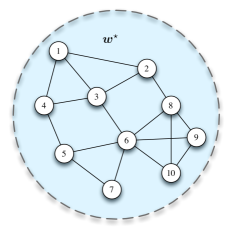
(a) Single-task network

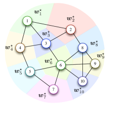
(b) Multitask network

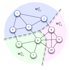
(c) Clustered multitask network

Figure 1: Three types of networks. The single-task and multitask networks can be viewed as special cases of the clustered multitask network.

III Problem formulation

III-A Global cost function and optimization

Clustered multitask networks require that nodes that are grouped in the same cluster estimate the same coefficient vector. Thus, consider the cluster ${\mathcal{C}}(k)$ to which node $k$ belongs. A local cost function, $J_{k}(\boldsymbol{w}_{{\mathcal{C}}(k)})$, is associated with node $k$ and it is assumed to be strongly convex and second-order differentiable, an example of which is the mean-square error criterion defined by

$$J_{k}(\boldsymbol{w}_{{\mathcal{C}}(k)})=E\left\{\big{|}d_{k}(n)-\boldsymbol{x}_{k}^{\top}(n)\,\boldsymbol{w}_{{\mathcal{C}}(k)}\big{|}^{2}\right\}.$$ (6)

In order to promote similarities among adjacent clusters, appropriate regularization can be used. For this purpose, we introduce the squared Euclidean distance as a possible regularizer, namely,

$$\Delta(\boldsymbol{w}_{{\mathcal{C}}(k)},\boldsymbol{w}_{{\mathcal{C}}(\ell)})=\|\boldsymbol{w}_{{\mathcal{C}}(k)}-\boldsymbol{w}_{{\mathcal{C}}(\ell)}\|^{2}.$$ (7)

Combining (6) and (7) yields the following regularized problem $\mathcal{P}_{1}$ at the level of the entire network:

$$(\mathcal{P}_{1})\qquad\overline{J^{\text{glob}}}(\boldsymbol{w}_{{\mathcal{C}}_{1}},\dots,\boldsymbol{w}_{{\mathcal{C}}_{Q}})=\sum_{k=1}^{N}E\left\{\big{|}d_{k}(n)-\boldsymbol{x}_{k}^{\top}(n)\,\boldsymbol{w}_{{\mathcal{C}}(k)}\big{|}^{2}\right\}+{\eta}\,\sum_{k=1}^{N}\sum_{\ell\in{\mathcal{N}}_{k}\backslash{\mathcal{C}}(k)}\rho_{k\ell}\,\|\boldsymbol{w}_{{\mathcal{C}}(k)}-\boldsymbol{w}_{{\mathcal{C}}(\ell)}\|^{2},$$ (8)

where $\boldsymbol{w}_{{\mathcal{C}}_{i}}$ is the parameter vector associated with cluster ${\mathcal{C}}_{i}$ and $\eta>0$. The second term on the right-hand-side of expression (8) promotes similarities between the $\boldsymbol{w}_{{\mathcal{C}}_{i}}$ of neighboring clusters, with strength parameter $\eta$.

Observe from the right-most term in (8) that the regularization strength between two clusters is directly related to the number of edges that connect them. The non-negative coefficients $\rho_{k\ell}$ aim at adjusting the regularization strength but they do not necessarily enforce symmetry. That is, we do not require $\rho_{k\ell}=\rho_{\ell k}$ even though the regularization term $\|\boldsymbol{w}_{{\mathcal{C}}(k)}-\boldsymbol{w}_{{\mathcal{C}}(\ell)}\|^{2}$ is symmetric with respect to the weight vectors $\boldsymbol{w}_{{\mathcal{C}}(k)}$ and $\boldsymbol{w}_{{\mathcal{C}}(\ell)}$; this term will be weighted by the sum $\rho_{k\ell}+\rho_{\ell k}$ due to the summation over the $N$ nodes. Consequently, problem formulation $\mathcal{P}_{1}$ inevitably leads to symmetric regularization despite the fact that $\rho_{k\ell}\neq\rho_{\ell k}$. However, we would like the design problem to benefit from the additional flexibility that is afforded by the use of asymmetric regularization coefficients. This is because asymmetry allows clusters to scale their desire for closer similarity with their neighbors differently. For example, asymmetric regularization would allow cluster ${\mathcal{C}}_{k}$ to promote similarities with cluster ${\mathcal{C}}_{\ell}$ while cluster ${\mathcal{C}}_{\ell}$ may be less inclined towards promoting similarities with ${\mathcal{C}}_{k}$. In order to exploit this flexibility more fully, we consider an alternative problem formulation $\mathcal{P}_{2}$ defined in terms of $Q$ Nash equilibrium problems as follows:

$$(\mathcal{P}_{2})\hskip 14.22636pt\left\{\begin{split}&\min_{\boldsymbol{w}_{{\mathcal{C}}_{i}}}\overline{J_{{\mathcal{C}}_{i}}}(\boldsymbol{w}_{{\mathcal{C}}_{i}},\boldsymbol{w}_{-{\mathcal{C}}_{i}})\qquad\text{for }i=1,\dots,Q\\ &\text{with }\;\overline{J_{{\mathcal{C}}_{i}}}(\boldsymbol{w}_{{\mathcal{C}}_{i}},\boldsymbol{w}_{-{\mathcal{C}}_{i}})=\sum_{k\in{\mathcal{C}}_{i}}E\left\{\big{|}d_{k}(n)-\boldsymbol{x}_{k}^{\top}(n)\,\boldsymbol{w}_{{\mathcal{C}}(k)}\big{|}^{2}\right\}+\eta\,\sum_{k\in{\mathcal{C}}_{i}}\sum_{\ell\in{\mathcal{N}}_{k}\backslash{\mathcal{C}}_{i}}\rho_{k\ell}\,\|\boldsymbol{w}_{{\mathcal{C}}(k)}-\boldsymbol{w}_{{\mathcal{C}}(\ell)}\|^{2}\end{split}\right.$$ (9)

where each cluster ${\mathcal{C}}_{i}$ estimates $\boldsymbol{w}_{{\mathcal{C}}_{i}}$ by minimizing $\overline{J_{{\mathcal{C}}_{i}}}(\boldsymbol{w}_{{\mathcal{C}}_{i}},\boldsymbol{w}_{-{\mathcal{C}}_{i}})$. Note that we have kept the notation $\boldsymbol{w}_{{\mathcal{C}}(k)}$ to make the role of the regularization term clearer, even though in formulation (9) we have $\boldsymbol{w}_{{\mathcal{C}}(k)}=\boldsymbol{w}_{{\mathcal{C}}_{i}}$ for all $k$ in ${\mathcal{C}}_{i}$. In (9), the notation $\boldsymbol{w}_{-{\mathcal{C}}_{i}}$ denotes the collection of weight vectors estimated by the other clusters, i.e., $\boldsymbol{w}_{-{\mathcal{C}}_{i}}=\{\boldsymbol{w}_{{\mathcal{C}}_{k}}:k=1,\ldots,Q\}-\{\boldsymbol{w}_{{\mathcal{C}}_{i}}\}$.

The Nash equilibrium of $\mathcal{P}_{2}$ satisfies the condition [Dynamic1995]:

$$\boldsymbol{w}_{{\mathcal{C}}_{i}}^{o}=\arg\min_{\boldsymbol{w}_{{\mathcal{C}}_{i}}}\overline{J_{{\mathcal{C}}_{i}}}(\boldsymbol{w}_{{\mathcal{C}}_{i}},\boldsymbol{w}^{o}_{-{\mathcal{C}}_{i}})$$ (10)

for $i=1,\dots,Q$, where the notation $\boldsymbol{w}^{o}_{-{\mathcal{C}}_{i}}$ denotes the collection of the Nash equilibria by the other clusters. Problem $\mathcal{P}_{2}$ has the following properties:

1. An equilibrium exists for $\mathcal{P}_{2}$ since $\overline{J_{{\mathcal{C}}_{i}}}(\boldsymbol{w}_{{\mathcal{C}}_{i}},\boldsymbol{w}_{-{\mathcal{C}}_{i}})$ is convex with respect to $\boldsymbol{w}_{{\mathcal{C}}_{i}}$ for all $i$.

2. The equilibrium for $\mathcal{P}_{2}$ is unique since $\{\overline{J_{{\mathcal{C}}_{i}}}(\boldsymbol{w}_{{\mathcal{C}}_{i}},\boldsymbol{w}_{-{\mathcal{C}}_{i}})\}_{i=1}^{Q}$ satisfies the diagonal strict convexity property.

3. Problems $\mathcal{P}_{1}$ and $\mathcal{P}_{2}$ have the same solution by setting the value of $\rho_{k\ell}$ in $\mathcal{P}_{2}$ to that of $\rho_{k\ell}+\rho_{\ell k}$ from $\mathcal{P}_{1}$.

Properties 1) and 2) can be checked via Theorems 1 and 2 in [rosen1965]. Property 3) can be verified by the optimality conditions for the two problems.

Problem $\mathcal{P}_{1}$ can be solved either analytically in closed form or iteratively by using a steepest-descent algorithm. Unfortunately, there is no analytical expression for general Nash equilibrium problems. We estimate the equilibrium of problem $\mathcal{P}_{2}$ iteratively by the fixed point of the best response iteration [Dynamic1995], that is,

$$\boldsymbol{w}_{{\mathcal{C}}_{i}}(n+1)=\arg\min_{\boldsymbol{w}_{{\mathcal{C}}_{i}}}\overline{J_{{\mathcal{C}}_{i}}}(\boldsymbol{w}_{{\mathcal{C}}_{i}},\boldsymbol{w}_{-{\mathcal{C}}_{i}}(n))$$ (11)

for $i=1,\dots,Q$, and leads to the solution of (9). Since the equilibrium is unique and the cost function for each cluster is convex, the solution of (9) can also be approached by means of a steepest-descent iteration as follows:

$$\boldsymbol{w}_{{\mathcal{C}}_{i}}(n+1)=\boldsymbol{w}_{{\mathcal{C}}_{i}}(n)-\mu\,\nabla_{\boldsymbol{w}_{{\mathcal{C}}_{i}}}\overline{J_{{\mathcal{C}}_{i}}}(\boldsymbol{w}_{{\mathcal{C}}_{i}}(n),\boldsymbol{w}_{-{\mathcal{C}}_{i}}(n))$$ (12)

for $i=1,\dots,Q$, with $\nabla_{\boldsymbol{w}_{{\mathcal{C}}_{i}}}$ denoting the gradient operation with respect to $\boldsymbol{w}_{{\mathcal{C}}_{i}}$, and $\mu$ a positive step-size. We have

$$\nabla_{\boldsymbol{w}_{{\mathcal{C}}_{i}}}\overline{J_{{\mathcal{C}}_{i}}}(\boldsymbol{w}_{{\mathcal{C}}_{i}},\boldsymbol{w}_{-{\mathcal{C}}_{i}}(n))\propto\sum_{k\in{\mathcal{C}}_{i}}(\boldsymbol{R}_{x,k}\boldsymbol{w}_{{\mathcal{C}}_{i}}-{\boldsymbol{p}}_{xd,k})+\eta\,\sum_{k\in{\mathcal{C}}_{i}}\sum_{\ell\in{\mathcal{N}}_{k}\backslash{\mathcal{C}}_{i}}\rho_{k\ell}\big{(}\boldsymbol{w}_{{\mathcal{C}}_{i}}-\boldsymbol{w}_{{\mathcal{C}}(\ell)}(n)\big{)}.$$ (13)

where $\boldsymbol{p}_{xd,k}=E\{\boldsymbol{x}_{k}(n)d_{k}(n)\}$ is the input-output cross-correlation vector between $\boldsymbol{x}_{k}(n)$ and $d_{k}(n)$ at node $k$. If some additional constraints are imposed on the parameters to estimate, the gradient update relation can be modified using methods such as projection [Theodoridis2011adap] or fixed point iteration techniques [chen2011nnlms]. In the body of the paper, we focus on the unconstrained case during the algorithm derivation and its analysis. However, a constrained problem will be presented in the simulation section. Since $\mathcal{P}_{1}$ is equivalent to $\mathcal{P}_{2}$ with proper setting of the weights $\rho_{k\ell}$, we shall now derive a distributed algorithm for solving problem $\mathcal{P}_{2}$. In this paper, we shall consider normalized weights that satisfy

$$\sum_{\ell=1}^{N}\rho_{k\ell}=1,\quad\text{and}\quad\rho_{k\ell}=0\;\text{ if }\,\ell\notin{\mathcal{N}}_{k}\backslash{\mathcal{C}}(k).$$ (14)

III-B Local cost decomposition and problem relaxation

The solution method (12) using (13) requires that every node in the network should have access to the statistical moments $\boldsymbol{R}_{x,k}$ and $\boldsymbol{p}_{xd,k}$ over its cluster. There are two problems with this scenario. First, nodes can only be assumed to have access to information from their immediate neighborhood and the cluster of every node $k$ may include nodes that are not direct neighbors of $k$. Second, nodes rarely have access to the moments $\{\boldsymbol{R}_{x,d},\boldsymbol{p}_{xd,k}\}$; instead, they have access to data generated from distributions with these moments. Therefore, more is needed to enable a distributed solution that relies solely on local interactions within neighborhoods and that relies on measured data as opposed to statistical moments. To derive a distributed algorithm, we follow the approach of [Cattivelli2010diff, Sayed2013intr]. The first step in this approach is to show how to express the cost (9) in terms of other local costs that only depend on data from neighborhoods.

Thus, let us introduce an $N\times N$ right stochastic matrix $\boldsymbol{C}$ with nonnegative entries $c_{\ell k}$ such that

$$\sum_{k=1}^{N}c_{\ell k}=1,\quad\text{and}\quad c_{\ell k}=0\,\text{ if }\,k\notin{\mathcal{N}}_{\ell}\cap{\mathcal{C}}(\ell).$$ (15)

With these coefficients, we associate a local cost function of the following form with each node $k$ [Sayed2013intr]:

$$J_{k}^{\text{loc}}(\boldsymbol{w}_{{\mathcal{C}}(k)})=\sum_{\ell\in{\mathcal{N}}_{k}\cap{\mathcal{C}}(k)}c_{\ell k}\,E\left\{\big{|}d_{\ell}(n)-\boldsymbol{x}_{\ell}^{\top}(n)\,\boldsymbol{w}_{{\mathcal{C}}(k)}\big{|}^{2}\right\}.$$ (16)

One important distinction from the local cost defined in [Sayed2013intr] is that in [Sayed2013intr] the summation in (16) is defined over the entire neighborhood of node $k$, i.e., for all $\ell\in{\mathcal{N}}_{k}$. Here we are excluding those neighbors of $k$ that do not belong to its cluster. This is because these particular neighbors will be pursuing a different parameter vector than node $k$. Furthermore, we note in (16) that $\boldsymbol{w}_{{\mathcal{C}}(k)}=\boldsymbol{w}_{{\mathcal{C}}(\ell)}$ because $\ell\in{\mathcal{C}}(k)$. To make the notation simpler, we shall write $\boldsymbol{w}_{k}$ instead of $\boldsymbol{w}_{{\mathcal{C}}(k)}$. A consequence of this notation is that $\boldsymbol{w}_{k}=\boldsymbol{w}_{\ell}$ for all $\ell\in{\mathcal{C}}(k)$. Incorporating the estimates of the neighboring clusters, we modify (16) to associate a regularized local cost function with node $k$ of the following form

$$\overline{J_{k}^{\text{loc}}}(\boldsymbol{w}_{k})=\sum_{\ell\in{\mathcal{N}}_{k}\cap{\mathcal{C}}(k)}c_{\ell k}\,E\left\{\big{|}d_{\ell}(n)-\boldsymbol{x}_{\ell}^{\top}(n)\,\boldsymbol{w}_{k}\big{|}^{2}\right\}+\eta\sum_{\ell\in{\mathcal{N}}_{k}\backslash{\mathcal{C}}(k)}\rho_{k\ell}\|\boldsymbol{w}_{k}-\boldsymbol{w}_{\ell}\|^{2}.$$ (17)

Observe that this local cost is now solely defined in terms of information that is available to node $k$ from its neighbors. Using this regularized local cost function, it can be verified that the global cost function for cluster ${\mathcal{C}}_{i}$ in (9) can be now expressed as

$$\overline{J_{{\mathcal{C}}_{i}}}(\boldsymbol{w}_{{\mathcal{C}}_{i}},\boldsymbol{w}_{-{\mathcal{C}}_{i}}) =\sum_{k\in{\mathcal{C}}_{i}}\Big{(}\sum_{\ell\in{\mathcal{C}}(k)}c_{\ell k}E\left\{\big{|}d_{\ell}(n)-\boldsymbol{x}_{\ell}^{\top}(n)\,\boldsymbol{w}_{{\mathcal{C}}(k)}\big{|}^{2}\right\}+\eta\,\sum_{\ell\in{\mathcal{N}}_{k}\backslash{\mathcal{C}}_{i}}\rho_{k\ell}\,\|\boldsymbol{w}_{{\mathcal{C}}(k)}-\boldsymbol{w}_{{\mathcal{C}}(\ell)}\|^{2}\Big{)}$$

$$=\sum_{k\in{\mathcal{C}}_{i}}\overline{J_{k}^{\text{loc}}}(\boldsymbol{w}_{k})$$

$$=\overline{J_{k}^{\text{loc}}}(\boldsymbol{w}_{k})+\sum_{\ell\in{\mathcal{C}}(k)\backslash k}\overline{J_{\ell}^{\text{loc}}}(\boldsymbol{w}_{\ell})$$ (18)

Let $\boldsymbol{w}_{k}^{o}$ denote the minimizer of the local cost function (17), given $\boldsymbol{w}_{\ell}$ for all $\ell\in{\mathcal{N}}_{k}\backslash{\mathcal{C}}(k)$. A completion-of-squares argument shows that each $\overline{J_{k}^{\text{loc}}}(\boldsymbol{w}_{k})$ can be expressed as

$$\overline{J_{k}^{\text{loc}}}(\boldsymbol{w}_{k})=\overline{J_{k}^{\text{loc}}}(\boldsymbol{w}_{k}^{o})+\|\boldsymbol{w}_{k}-\boldsymbol{w}_{k}^{o}\|^{2}_{\overline{\boldsymbol{R}}_{k}}$$ (19)

where

$$\overline{\boldsymbol{R}}_{k}=\sum_{\ell\in{\mathcal{N}}_{k}\cap{\mathcal{C}}(k)}c_{\ell k}\,\boldsymbol{R}_{x,\ell}+\eta\sum_{\ell\in{\mathcal{N}}_{k}\backslash{\mathcal{C}}(k)}\rho_{k\ell}\boldsymbol{I}_{L}.$$ (20)

Substituting equation (19) into the second term on the right-hand-side of (18), and discarding the terms $\{\overline{J_{\ell}^{\text{loc}}}(\boldsymbol{w}_{\ell}^{o})\}$because they are independent of the optimization variables in the cluster, we can consider the following equivalent cost function for cluster ${\mathcal{C}}(k)$ at node $k$:

$$\overline{J_{{\mathcal{C}}(k)}}(\boldsymbol{w}_{k})\triangleq\overline{J_{k}^{\text{loc}}}(\boldsymbol{w}_{k})+\sum_{\ell\in{\mathcal{C}}(k)\backslash k}\|\boldsymbol{w}_{\ell}-\boldsymbol{w}^{o}_{\ell}\|^{2}_{\overline{\boldsymbol{R}}_{\ell}}$$ (21)

where it holds that $\boldsymbol{w}_{k}=\boldsymbol{w}_{\ell}$ because $\ell\in{\mathcal{C}}(k)$. Note that we have omitted $\boldsymbol{w}_{-k}$ in the notation for $\overline{J_{{\mathcal{C}}(k)}}(\boldsymbol{w}_{k})$ for the sake of brevity. Therefore, minimizing (21) is equivalent to minimizing the original cost (18) or (9) over $\boldsymbol{w}_{k}$. However the second term (21) still requires information from nodes $\ell$ that may not be in the direct neighborhood of node $k$ even though they belong to the same cluster. In order to avoid access to information via multi-hop, we can relax the cost function (21) at node $k$ by considering only information originating from its neighbors. This can be achieved by replacing the range of the index over which the summation in (21) is computed as follows:

$$\overline{J_{{\mathcal{C}}(k)}}^{\prime}(\boldsymbol{w}_{k})=\overline{J_{k}^{\text{loc}}}(\boldsymbol{w}_{k})+\sum_{\ell\in{\mathcal{N}}_{k}^{-}\cap{\mathcal{C}}(k)}\|\boldsymbol{w}_{k}-\boldsymbol{w}^{o}_{\ell}\|^{2}_{\overline{\boldsymbol{R}}_{\ell}}.$$ (22)

Usually, especially in the context of adaptive learning in a non-stationary environment, the weighting matrices $\overline{\boldsymbol{R}_{\ell}}$ are unavailable since the covariance matrices $\boldsymbol{R}_{x,\ell}$ at each node may not be known beforehand. Following an argument based on the Rayleigh-Ritz characterization of eigenvalues, it was explained in [Sayed2013intr] that a useful strategy is to replace each matrix $\overline{\boldsymbol{R}}_{\ell}$ by a weighted multiple of the identity matrix, say, as:

$$\|\boldsymbol{w}_{k}-\boldsymbol{w}^{o}_{\ell}\|^{2}_{\overline{\boldsymbol{R}}_{\ell}}\approx{b_{\ell k}}\,\|\boldsymbol{w}_{k}-\boldsymbol{w}^{o}_{\ell}\|^{2}$$ (23)

for some nonnegative coefficients $b_{\ell k}$ that can possibly depend on the node $k$. As shown later, these coefficients will be incorporated into a left stochastic matrix to be defined and, therefore, the designer does not need to worry about the selection of the $b_{\ell k}$ at this stage. Based on the arguments presented so far, and using (17), the global cost function (22) can then be relaxed to the following form:

$$\begin{split}\overline{J_{{\mathcal{C}}(k)}}^{\prime\prime}(\boldsymbol{w}_{k})=\sum_{\ell\in{\mathcal{N}}_{k}\cap{\mathcal{C}}(k)}c_{\ell k}&\,E\left\{\big{|}d_{\ell}(n)-\boldsymbol{x}_{\ell}^{\top}(n)\,\boldsymbol{w}_{k}\big{|}^{2}\right\}\\ &+\eta\sum_{\ell\in{\mathcal{N}}_{k}\backslash{\mathcal{C}}(k)}\rho_{k\ell}\,\|\boldsymbol{w}_{k}-\boldsymbol{w}_{\ell}\|^{2}+\sum_{\ell\in{\mathcal{N}}_{k}^{-}\cap{\mathcal{C}}(k)}{b_{\ell k}}\|\boldsymbol{w}_{k}-\boldsymbol{w}^{o}_{\ell}\|^{2}.\end{split}$$ (24)

Observe that the two last sums on the right-hand-side of (24) divide the neighbors of node $k$ into two exclusive sets: those that belong to its cluster (last sum) and those that do not belong to its cluster (second term). In summary, the argument so far enabled us to replace the cost (9) by the alternative cost (24) that depends only on data within the neighborhood of node $k$. We can now proceed to use (24) to derive distributed strategies. Subsequently, we study the stability and mean-square performance of the resulting strategies and show that they are able to perform well despite the approximation introduced in steps.

IV Stochastic approximation algorithms

To begin with, a steepest-descent iteration can be applied by each node $k$ to minimize the cost function (24). Let $\boldsymbol{w}_{k}(n)$ denote the estimate for $\boldsymbol{w}_{k}$ at iteration $n$. Using a constant step-size $\mu$ for each node, the update relation would take the following form:

$$\begin{split}\boldsymbol{w}_{k}(n+1)=\boldsymbol{w}_{k}(n)&-\mu\sum_{\ell\in{\mathcal{N}}_{k}\cap{\mathcal{C}}(k)}c_{\ell k}\left(\boldsymbol{R}_{x,\ell}\boldsymbol{w}_{k}(n)-{\boldsymbol{p}}_{xd,k}\right)-\mu\eta\sum_{\ell\in{\mathcal{N}}_{k}\backslash{\mathcal{C}}(k)}\rho_{k\ell}\,\left(\boldsymbol{w}_{k}(n)-\boldsymbol{w}_{\ell}(n)\right)\\ &-\mu\sum_{\ell\in{{\mathcal{N}}_{k}^{-}\cap{\mathcal{C}}(k)}}b_{\ell k}\,\left(\boldsymbol{w}_{k}(n)-\boldsymbol{w}^{o}_{\ell}\right)\end{split}$$ (25)

Among other possible forms, expression (25) can be evaluated in two successive update steps

$$\boldsymbol{\psi}_{k}(n+1)=\boldsymbol{w}_{k}(n)-\mu\left(\sum_{\ell\in{\mathcal{N}}_{k}\cap{\mathcal{C}}(k)}c_{\ell k}\left(\boldsymbol{R}_{x,\ell}\boldsymbol{w}_{k}(n)-{\boldsymbol{p}}_{xd,k}\right)+\eta\sum_{\ell\in{\mathcal{N}}_{k}\backslash{\mathcal{C}}(k)}\rho_{k\ell}\,(\boldsymbol{w}_{k}(n)-\boldsymbol{w}_{\ell}(n))\right)$$ (26)

$$\boldsymbol{w}_{k}(n+1)=\boldsymbol{\psi}_{k}(n+1)+\mu\sum_{\ell\in{{\mathcal{N}}_{k}^{-}\cap{\mathcal{C}}(k)}}b_{\ell k}\,\left(\boldsymbol{w}^{o}_{\ell}-\boldsymbol{w}_{k}(n)\right)$$ (27)

Following the same line of reasoning from [Sayed2013intr] in the single-task case, and extending the argument to apply to clusters, we use $\boldsymbol{\psi}_{\ell}(n+1)$ as a local estimate for $\boldsymbol{w}^{o}_{\ell}$ in (27) since the latter is unavailable and $\boldsymbol{\psi}_{\ell}(n+1)$ is an intermediate estimate for it that is available at node $\ell$ at time $n+1$. In addition, again in step (27), we replace $\boldsymbol{w}_{k}(n)$ by $\boldsymbol{\psi}_{k}(n+1)$ since it is a better estimate obtained by incorporating information from the neighbors according to (26). Step (27) then becomes

$$\boldsymbol{w}_{k}(n+1)=\left(1-\mu\sum_{\ell\in{{\mathcal{N}}_{k}^{-}\cap{\mathcal{C}}(k)}}b_{\ell k}\right)\boldsymbol{\psi}_{k}(n+1)+\mu\sum_{\ell\in{{\mathcal{N}}_{k}^{-}\cap{\mathcal{C}}(k)}}b_{\ell k}\,\boldsymbol{\psi}_{\ell}(n+1).$$ (28)

The coefficients in (28) can be redefined as:

$$\begin{split}a_{kk}&\triangleq 1-\mu\sum_{\ell\in{{\mathcal{N}}_{k}^{-}\cap{\mathcal{C}}(k)}}b_{\ell k}\\ a_{\ell k}&\triangleq\mu\,b_{\ell k},\quad\ell\in{\mathcal{N}}_{k}^{-}\cap{\mathcal{C}}(k)\\ a_{\ell k}&\triangleq 0,\quad\ell\notin{\mathcal{N}}_{k}\cap{\mathcal{C}}(k)\end{split}$$ (29)

It can be observed that the entries $\{a_{\ell k}\}$ are nonnegative for all $\ell$ and $k$ (including $a_{kk}$) for sufficiently small step-size. Moreover, the matrix $\boldsymbol{A}$ with ($\ell,k$)-th entry $a_{\ell k}$ is a left-stochastic matrix, which means that the sum of each of its columns is equal to one. With this notation, we obtain the following adapt-then-combine (ATC) diffusion strategy for solving problem (9) in a distributed manner:

$$\begin{split}&\boldsymbol{\psi}_{k}(n+1)=\boldsymbol{w}_{k}(n)-\mu\,\left(\sum_{\ell\in{\mathcal{N}}_{k}\cap{\mathcal{C}}(k)}c_{\ell k}\left(\boldsymbol{R}_{x,\ell}\boldsymbol{w}_{k}(n)-{\boldsymbol{p}}_{xd,k}\right)+\eta\sum_{\ell\in{\mathcal{N}}_{k}\backslash{\mathcal{C}}(k)}\rho_{k\ell}\,(\boldsymbol{w}_{k}(n)-\boldsymbol{w}_{\ell}(n))\right)\\ &\boldsymbol{w}_{k}(n+1)=\sum_{\ell\in{\mathcal{N}}_{k}\cap{\mathcal{C}}(k)}a_{\ell k}\,\boldsymbol{\psi}_{k}(n+1)\end{split}$$ (30)

At each instant $n+1$, node $k$ updates the intermediate value $\boldsymbol{\psi}_{k}(n+1)$ with a local steepest descent iteration. This step involves a regularization term in the case where the set of inter-cluster neighbors of node $k$ is not empty. Next, an aggregation step is performed where node $k$ combines its intermediate value $\boldsymbol{\psi}_{k}(n+1)$ with the intermediate values $\boldsymbol{\psi}_{\ell}(n+1)$ from its cluster neighbors. It is also possible to arrive at a combine-then-adapt (CTA) diffusion strategy where the aggregation step is performed prior to the adaptation step [Sayed2013intr]. In what follows, it is sufficient to focus on the ATC strategy to illustrate the main results. Employing instantaneous approximations for the required signal moments in (30), we arrive at the desired diffusion strategy for clustered multitask learning described in Algorithm 1 where the regularization factors $\rho_{k\ell}$ are chosen according to (14), and the coefficients $\{c_{\ell k},a_{\ell k}\}$ are nonnegative scalars chosen at will by the designer to satisfy the following conditions:

$$a_{\ell k}\geq 0,\;\;\;\sum_{\ell\in{\cal N}_{k}\cap{\cal C}(k)}a_{\ell k}=1,\;\;\;a_{\ell k}=0\;\;\mbox{\rm for }\;\ell\notin{\cal N}_{k}\cap{\cal C}(k)$$ (31)

$$c_{\ell k}\geq 0,\;\;\;\sum_{k\in{\cal N}_{\ell}\cap{\cal C}(\ell)}c_{\ell k}=1,\;\;\;c_{\ell k}=0\;\;\mbox{\rm for }\;k\notin{\cal N}_{\ell}\cap{\cal C}(\ell)$$ (32)

There are several ways to select these coefficients such as using the averaging rule or the Metropolis rule (see [Sayed2013intr] for a listing of these and other choices).

Start with $\boldsymbol{w}_{k}(0)=0$ for all $k$, and repeat:

$$\left\{\begin{split}&\boldsymbol{\psi}_{k}(n+1)=\boldsymbol{w}_{k}(n)+\mu\left(\sum_{\ell\in{\mathcal{N}}_{k}\cap{\mathcal{C}}(k)}c_{\ell k}\left(d_{\ell}(n)-\boldsymbol{x}_{\ell}^{\top}(n)\boldsymbol{w}_{k}(n)\right)\boldsymbol{x}_{\ell}(n)+\eta\sum_{\ell\in{\mathcal{N}}_{k}\backslash{\mathcal{C}}(k)}\rho_{k\ell}\,(\boldsymbol{w}_{\ell}(n)-\boldsymbol{w}_{k}(n))\right)\\ &\boldsymbol{w}_{k}(n+1)=\sum_{\ell\in{\mathcal{N}}_{k}\cap{\mathcal{C}}(k)}a_{\ell k}\,\boldsymbol{\psi}_{k}(n+1)\end{split}\right.$$ (33)

Algorithm 1 Diffusion LMS for clustered multitask networks

In the case of a single-task network when there is a single cluster that consists of the entire set of nodes we get ${\mathcal{N}}_{k}\cap\,{\mathcal{C}}(k)={\mathcal{N}}_{k}$ and ${\mathcal{N}}_{k}\backslash{\mathcal{C}}(k)=\emptyset$ for all $k$, so that expression (33) reduces to the diffusion adaptation strategy [Sayed2013intr, Cattivelli2010diff] described in Algorithm 2.

Start with $\boldsymbol{w}_{k}(0)=0$ for all $k$, and repeat:

$$\left\{\begin{split}&\boldsymbol{\psi}_{k}(n+1)=\boldsymbol{w}_{k}(n)+\mu\!\sum_{\ell\in{\mathcal{N}}_{k}}\!\!c_{\ell k}\left(d_{\ell}(n)-\boldsymbol{x}_{\ell}^{\top}(n)\boldsymbol{w}_{k}(n)\right)\boldsymbol{x}_{\ell}(n)\\ &\boldsymbol{w}_{k}(n+1)=\sum_{\ell\in{\mathcal{N}}_{k}}a_{\ell k}\,\boldsymbol{\psi}_{k}(n+1)\end{split}\right.$$ (34)

Algorithm 2 Diffusion LMS for single-task networks [Lopes2008diff, Cattivelli2010diff].

In the case of a multitask network where the size of each cluster is one, we have ${\mathcal{N}}_{k}\cap{\mathcal{C}}(k)=\{k\}$ and ${\mathcal{N}}_{k}\backslash{\mathcal{C}}(k)={\mathcal{N}}_{k}^{-}$ for all $k$, the algorithm and (34) degenerate into Algorithm 3. Interestingly, this is the instantaneous gradient counterpart of equation (12) for each node.

Start with $\boldsymbol{w}_{k}(0)=0$ for all $k$, and repeat:

$$\boldsymbol{w}_{k}(n+1)=\boldsymbol{w}_{k}(n)+\mu\,\left(d_{k}(n)-\boldsymbol{x}_{k}^{\top}(n)\boldsymbol{w}_{k}(n)\right)\boldsymbol{x}_{k}(n)+\eta\,\mu\sum_{\ell\in{\mathcal{N}}_{k}^{-}}\rho_{k\ell}\left(\boldsymbol{w}_{\ell}(n)-\boldsymbol{w}_{k}(n)\right)$$ (35)

Algorithm 3 Diffusion LMS for multitask networks

V Mean-Square Error Performance Analysis

We now examine the stochastic behavior of the adaptive diffusion strategy (33). In order to address this question, we collect information from across the network into block vectors and matrices. In particular, let us denote by $\boldsymbol{w}(n)$, $\boldsymbol{w}^{\star}$ and $\boldsymbol{\psi}$ the block weight estimate vector, the block optimum weight vector and block intermediate weight estimate vector, all of size $LN\times 1$, i.e.,

$$\boldsymbol{w}(n)=\left(\begin{array}[]{c}\boldsymbol{w}_{1}(n)\\ \vdots\\ \boldsymbol{w}_{N}(n)\end{array}\right),\qquad\qquad\boldsymbol{w}^{\star}=\left(\begin{array}[]{c}\boldsymbol{w}^{\star}_{1}\\ \vdots\\ \boldsymbol{w}^{\star}_{N}\end{array}\right),\qquad\qquad\boldsymbol{\psi}(n)=\left(\begin{array}[]{c}\boldsymbol{\psi}_{1}(n)\\ \vdots\\ \boldsymbol{\psi}_{N}(n)\end{array}\right)$$ (36)

with $\boldsymbol{w}^{\star}_{k}=\boldsymbol{w}^{\star}_{{\mathcal{C}}(k)}$. The weight error vector for each node $k$ at iteration $n$ is defined by $\boldsymbol{v}_{k}(n)=\boldsymbol{w}_{k}(n)-\boldsymbol{w}^{\star}_{k}$. The weight error vectors $\boldsymbol{v}_{k}(n)$ are also stacked on top of each other to get the block weight error vector defined as follows:

$$\boldsymbol{v}(n)=\left(\begin{array}[]{c}\boldsymbol{v}_{1}(n)\\ \vdots\\ \boldsymbol{v}_{N}(n)\end{array}\right)$$ (37)

To perform the theoretical analysis, we introduce the following independence assumption.

Assumption 1

(Independent regressors) The regression vectors $\boldsymbol{x}_{k}(n)$ arise from a stationary random process that is temporally stationary, white and independent over space with $\boldsymbol{R}_{x,k}=E\{\boldsymbol{x}_{k}(n)\boldsymbol{x}^{\top}_{k}(n)\}>0$.

A direct consequence is that $\boldsymbol{x}_{k}(n)$ is independent of $\boldsymbol{v}_{\ell}(m)$ for all $\ell$ and $m\leq n$. Although not true in general, this assumption is commonly used for analyzing adaptive constructions because it allows to simplify the derivations without constraining the conclusions. Moreover, various analyses in the literature have already shown that performance results obtained under this assumption match well the actual performance of adaptive algorithms when the step-size is sufficiently small [sayed2008adaptive].

V-A Mean error behavior analysis

The estimation error that appears in the first equation of (33) can be rewritten as

$$\begin{split}d_{\ell}(n)-\boldsymbol{x}_{\ell}^{\top}(n)\boldsymbol{w}_{k}(n)&=\boldsymbol{x}_{\ell}^{\top}(n)\boldsymbol{w}_{k}^{\star}+z_{\ell}(n)-\boldsymbol{x}_{\ell}^{\top}(n)\boldsymbol{w}_{k}(n)\\ &=z_{\ell}(n)-\boldsymbol{x}_{\ell}^{\top}(n)\boldsymbol{v}_{k}(n)\end{split}$$ (38)

because $\boldsymbol{w}_{\ell}^{\star}=\boldsymbol{w}_{k}^{\star}$ for all $\ell\in{\mathcal{N}}_{k}\cap{\mathcal{C}}(k)$. Subtracting $\boldsymbol{w}^{\star}_{k}$ from both sides of the first equation in (33), and using the above relation, the update equation for the block weight error vector of $\boldsymbol{\psi}_{k}(n+1)$ can be expressed as

$$\boldsymbol{\psi}(n+1)-\boldsymbol{w}^{\star}=\boldsymbol{v}(n)-\mu\,\boldsymbol{H}_{x}(n)\,\boldsymbol{v}(n)+\mu\,\boldsymbol{p}_{zx}(n)-\mu\,\eta\,\boldsymbol{Q}\,(\boldsymbol{v}(n)+\boldsymbol{w}^{\star})$$ (39)

where

$$\boldsymbol{Q}=\boldsymbol{I}_{LN}-\boldsymbol{P}\otimes\boldsymbol{I}_{L},$$ (40)

with $\otimes$ denoting the Kronecker product, and $\boldsymbol{P}$ the $N\times N$ matrix with $(k,\ell)$-th entry $\rho_{k\ell}$. Moreover, the matrix $\boldsymbol{H}_{x}(n)$ is block diagonal of size $LN\times LN$ defined as

$$\boldsymbol{H}_{x}(n)=\text{diag}\Big{\{}\sum_{\ell\in{\mathcal{N}}_{1}\cap{\mathcal{C}}(1)}c_{\ell 1}\,\boldsymbol{x}_{\ell}(n)\boldsymbol{x}_{\ell}^{\top}(n),\,\dots,\!\!\!\sum_{\ell\in{\mathcal{N}}_{N}\cap{\mathcal{C}}(N)}c_{\ell N}\,\boldsymbol{x}_{\ell}(n)\boldsymbol{x}_{\ell}^{\top}(n)\Big{\}},$$ (41)

and $\boldsymbol{p}_{zx}(n)$ is the following vector of length $LN\times 1$:

$$\boldsymbol{p}_{zx}(n)=\Big{(}\sum_{\ell\in{\mathcal{N}}_{1}\cap{\mathcal{C}}(1)}c_{\ell 1}\,\boldsymbol{x}_{\ell}^{\top}(n)z_{\ell}(n),\,\dots,\!\!\!\sum_{\ell\in{\mathcal{N}}_{N}\cap{\mathcal{C}}(N)}c_{\ell N}\,\boldsymbol{x}_{\ell}^{\top}(n)z_{\ell}(n)\Big{)}^{\top}.$$ (42)

Let ${\boldsymbol{A}}_{I}=\boldsymbol{A}\otimes\boldsymbol{I}_{L}$. The second equation in (33) then allows us to write

$$\boldsymbol{w}(n+1)=\boldsymbol{A}_{I}^{\top}\,\boldsymbol{\psi}(n+1)$$ (43)

Subtracting $\boldsymbol{w}^{\star}$ from both sides of the above expression, and using equation (39), the update relation can be written in a single expression as follows

$$\begin{split}\boldsymbol{v}(n+1)=\boldsymbol{A}_{I}^{\top}\left[\boldsymbol{I}_{LN}-\mu\,(\boldsymbol{H}_{x}(n)+\eta\,\boldsymbol{Q})\right]\,\boldsymbol{v}(n)+\mu\,\boldsymbol{A}_{I}^{\top}\,\boldsymbol{p}_{zx}(n)-\mu\,\eta\,\boldsymbol{A}_{I}^{\top}\boldsymbol{Q}\,\boldsymbol{w}^{\star}\end{split}$$ (44)

Taking the expectation of both sides, and using Assumption 1 we get

$$E\{\boldsymbol{v}(n+1)\}=\boldsymbol{A}_{I}^{\top}\left[\boldsymbol{I}_{LN}-\mu\,(\boldsymbol{H}_{R}+\eta\,\boldsymbol{Q})\right]\,E\{\boldsymbol{v}(n)\}-\mu\,\eta\,\boldsymbol{A}_{I}^{\top}\boldsymbol{Q}\,\boldsymbol{w}^{\star}$$ (45)

where

$$\boldsymbol{H}_{R}\triangleq E\{\boldsymbol{H}_{x}(n)\}=\text{diag}\left\{\boldsymbol{R}_{1},\,\dots,\boldsymbol{R}_{N}\right\}$$ (46)

with

$$\boldsymbol{R}_{k}=\sum_{\ell\in{\mathcal{N}}_{k}\cap{\mathcal{C}}(k)}c_{\ell k}\,\boldsymbol{R}_{x,\ell}.$$ (47)