The top quark induced backgrounds to Higgs production in the $WW^{(*)}\to ll\nu\nu$ decay channel at NLO in QCD

Abstract

We present the complete NLO contributions to the $pp\to e^{+}\nu_{e}\mu^{-}\bar{\nu}_{\mu}b\bar{b}+X$ process in the four flavour scheme, i.e. with massive b quarks, and its contribution to the $H\to WW^{(*)}\to ll\nu\nu$ measurement in the 1-jet bin at the LHC. This background process includes top pair, single top and non-top quark-resonant contributions. The uncertainty at NLO from renormalisation and factorisation scale dependence is about ${+30}\%\,\,{-20}\%$. We show that the NLO corrections are relatively small, and that separating this background in top pair, $Wt$ and $b$-quark associated $ll\nu\nu$ production is a fair approximation.

After the Higgs boson discovery Aad et al. (2012); Chatrchyan et al. (2012a) the next step is to determine whether this boson is (solely) responsible for the electroweak symmetry breaking and for generating the masses of all the fundamental particles. The way to tackle this is to extract the coupling constants of the Higgs boson by measuring the Higgs boson cross sections in as many production and decay modes as possible.

For the discovery of the Higgs boson the three most important channels were the $H\to\gamma\gamma$, $H\to ZZ^{(*)}\to 4l$ and $H\to WW^{(*)}\to ll\nu\nu$ decay modes. Even though the latter has the largest branching ratio, it has the smallest contribution to the Higgs signal significance. This comes as no surprise: due to the presence of two neutrinos in the final state, the reconstruction of the Higgs signal in the form of a narrow resonance peak over a flat background is not possible for this decay mode. This makes the separation of the Higgs signal from (non) reducible backgrounds much more complicated and precise predictions for the backgrounds are needed to determine the excess of events that can be attributed to the Higgs signal.

To increase the significance in the extraction of the Higgs contribution for the $H\to WW^{(*)}\to ll\nu\nu$ channel, the data is separated in jet bins by the CMS and ATLAS experiments Chatrchyan et al. (2012b); ATL (2013). In the 0-jet bin, the dominant background is the non-reducible $pp\to WW$ production. In the 1-jet bin, where each event is required to have exactly 1 jet in association with the two charged leptons and the missing $E_{T}$, also the backgrounds from top quarks are large; mostly top pair and $Wt$ production. For a reliable simulation of these backgrounds, including next-to-leading order (NLO) QCD corrections in the calculation is essential. In this letter, we present the top induced background to Higgs production in the 1-jet bin, without separating top pair and $Wt$ production and thus keeping all their interference effects. This requires the calculation of the NLO corrections to the $pp\to e^{+}\nu_{e}\mu^{-}\bar{\nu}_{\mu}b\bar{b}+X$ process in the four-flavour (4F) scheme, keeping the $b$ quark mass finite, which we present here for the first time.

The NLO corrections to the $pp\to e^{+}\nu_{e}\mu^{-}\bar{\nu}_{\mu}b\bar{b}+X$ process in the five-flavour (5F) scheme are known Denner et al. (2011); Bevilacqua et al. (2011); Denner et al. (2012). In the 5F scheme the mass of the $b$ quark is neglected, which means that the above process is not finite in fixed-order perturbation theory without requiring phase-space cuts on the final state $b$ jets. Therefore, such a calculation cannot be used to estimate the $Wt$ and top pair production processes and, moreover, it cannot be used to estimate the top background in the 1-jet bin in the $H\to WW^{(*)}\to ll\nu\nu$ measurement, where a veto on a second jet is needed.

The calculation of the $pp\to e^{+}\nu_{e}\mu^{-}\bar{\nu}_{\mu}b\bar{b}+X$ process in the 4F scheme includes double top-quark resonant production (“top pair production”), single top-quark resonant contributions (“$W$ boson associated single top production”) as well as non top-quark resonant contributions ( “$b$-quark associated $ll\nu\nu$ production”). In Fig. 1 three representative LO Feynman diagrams are shown for this process. The calculation includes all the interference effects between the various contributions, as well as all off-shell effects. In the 4F scheme the $b$ quarks are treated as massive particles, the running of the strong coupling is performed with four flavours and a 4F PDF set should be used. Keeping the $b$ quark massive in the calculation implies that even in the absence of any phase-space cuts, the perturbative expansion yields finite results. For the NLO computation presented here, the complete $\mathcal{O}(\alpha_{s})$ corrections have been included without resorting to any approximations.

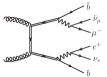
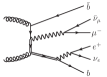
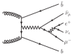
Figure 1: Representative LO diagrams for top pair (a), $Wt$ (b) and $b$-quark associated $ll\nu\nu$ (c) contributions to $pp\to e^{+}\nu_{e}\mu^{-}\bar{\nu}_{\mu}b\bar{b}+X$ production. Top quarks are denoted by double fermion lines.

The calculation has been performed within the MadGraph5_aMC@NLO framework Frederix et al. (2013): the diagram generation is done by MadGraph Alwall et al. (2011), the one-loop corrections are obtained with MadLoop Hirschi et al. (2011), which is based on the OPP reduction method Ossola et al. (2007) and its implementation in CutTools Ossola et al. (2008) and uses the OpenLoop algorithm Cascioli et al. (2012). The phase-space integration and the cancellation of IR divergences in intermediate steps of the calculation are dealt with by MadFKS Frederix et al. (2009), which is based on the FKS subtraction method Frixione et al. (1996). Furthermore, we use the complex mass scheme Denner et al. (1999, 2005), as implemented in MadGraph5_aMC@NLO Buarque Franzosi et al. (2013), for the treatment of the widths of heavy resonances. The implementation of the various contributions in the MadGraph5_aMC@NLO program is done in a completely process-independent way and allows for complete automation of the calculation with extensively tested algorithms, which minimises the possibility of computational errors.

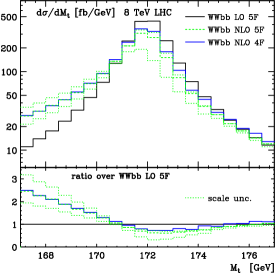
Figure 2: Top quark invariant mass computed by taking the invariant mass of the positron, electron-neutrino and the jet containing the $b$ quark, using the same parameters and cuts as in Ref. Denner et al. (2012) for the $pp\to e^{+}\nu_{e}\mu^{-}\bar{\nu}_{\mu}b\bar{b}+X$ process. The LO (black solid) and NLO (green dashed) predictions in the 5F scheme and NLO in the 4F scheme (blue solid) are plotted. The green dotted lines show the scale uncertainty on the NLO 5F result.

As a further check on the implementation of the various algorithms in the MadGraph5_aMC@NLO program, we have compared the results obtained in the 5F scheme by Denner et al. in Ref. Denner et al. (2012) by a 5F scheme calculation obtained within our framework and found excellent agreement. As an example, in Fig. 2 we show the positron–electron-neutrino–$b$-jet invariant mass, using exactly the same cuts and parameters as used in Ref. Denner et al. (2012); thus this plot can be directly compared to Fig. 16 of that reference. In the plot, we also present the same observable simulated in the 4F scheme, i.e. the calculation presented for the first time in this letter. The 4F and 5F scheme results lie (almost) exactly on top of each other for $M_{t}<172\,\textrm{GeV}$, where the shape is dominated by resonant contributions ($M_{t}\simeq 172\,\textrm{GeV}$) in which some radiation from the bottom quark is not clustered in the $b$ jet. The region $M_{t}>172\,\textrm{GeV}$ is more sensitive to the exact treatment of the (non)-resonant contributions Papanastasiou et al. (2013), but also here the differences between 4F and 5F scheme calculation are small and their respective scale uncertainty bands overlap. (Uncertainty band for the 4F scheme calculation is not shown).

To predict the top induced backgrounds in the $H\to WW^{(*)}\to ll\nu\nu$ decay channel at the 8 TeV LHC we use the following parameters. The mass of the top quark is set to $m_{t}=172\,\textrm{GeV}$, the mass of the bottom quark is $m_{b}=4.7\,\textrm{GeV}$ and the mass of the $W$ and $Z$ bosons are $m_{W}=80.399\,\textrm{GeV}$ and $m_{Z}=91.188\,\textrm{GeV}$. The (inverse of the) weak coupling is set to $\alpha^{-1}=132.35$. The width of the $W$ and $Z$ bosons are $\Gamma_{W}=2.100\,\textrm{GeV}$ and $\Gamma_{Z}=2.510\,\textrm{GeV}$, respectively. At LO the top width is set to $\Gamma_{t}^{\textrm{LO}}=1.44\,\textrm{GeV}$ and at NLO we use $\Gamma_{t}^{\textrm{NLO}}=1.32\,\textrm{GeV}$. For the description of the partons inside the colliding protons, the 4F MSTW2008nf4(N)LO PDF sets Martin et al. (2009) are used for the (N)LO calculation. This also defines the numerical value and running of the strong coupling constant.

We impose the following “Higgs measurement” cuts on the final state particles, which are are motivated by the cut-based analysis for the ATLAS measurement of the Higgs boson in the $WW^{(*)}\to ll\nu\nu$ decay channel ATL (2013). We require two charged leptons in the central rapidity region, $|\eta_{l}|<2.4$, of which the hardest needs to have a transverse momentum $p_{T}^{\textrm{lead}}>25$ GeV and the other a $p_{T}^{\textrm{sublead}}>15$ GeV. The lepton invariant mass should be larger than $m_{ll}>10$ GeV. We require exactly one jet with $|\eta_{j}|<4.7$, defined using the anti-$k_{T}$ algorithm Cacciari et al. (2008) with $\Delta R=0.5$ and a minimal transverse energy of $E_{T}^{j}>30$ GeV, where $E_{T}=\sqrt{m^{2}+p_{T}^{2}}$. Furthermore, there should be a sizeable (relative) missing transverse energy $E_{T,\textrm{rel}}^{\textrm{miss}}>25$ GeV, where $E_{T,\textrm{rel}}^{\textrm{miss}}=s\,E_{T}^{\textrm{miss}}$, with $E_{T}^{\textrm{miss}}$ the usual missing transverse energy and $s=\sin|\Delta\phi_{\textrm{closest}}|$, i.e. the sinus of the azimuthal separation between the missing transverse momentum vector and the closest charged lepton or the jet if there is one in the same azimuthal hemisphere. If there is no such object, $s=1$. The MC truth is used to define the missing transverse energy vector as the (transverse part of the) sum of the two neutrino momenta. Finally, the following $H\to WW^{(*)}\to l\nu l\nu$ topology cuts are applied: the lepton invariant mass should be smaller than $m_{ll}<50$ GeV and their azimuthal separation smaller than $|\Delta\phi_{ll}|<1.8$.

Due to the complexity of the process, and the rather involved set of cuts, it is not straight-forward to define a single hard scale for this process that could be used as a renormalisation and factorisation scale. We have therefore chosen a scale that is not very specific to this process, but should capture well the general hardness of the kinematics. This central scale is $\mu_{R}^{0}=\mu_{F}^{0}=H_{T}/2$, i.e. half the scalar sum of the transverse energies of all the final state particles/partons (including the two neutrinos). With this central scale, NLO corrections are relatively small for both the inclusive process as well as after applying the cuts described above. To assess contributions from beyond NLO we assign an uncertainty to our predictions by computing the envelope of the results with renormalisation and factorisation scales equal to $(\mu_{R},\mu_{F})=\{(1,1),(0.5,0.5),(2,2),(0.5,1),(2,1),(1,0.5),(1,2)\}\times(\mu_{R}^{0},\mu_{F}^{0})$. These 7 values are obtained at no extra CPU cost using the reweighting method described in Ref. Frederix et al. (2012).

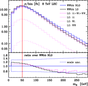
Figure 3: Invariant mass of the charged lepton pair for the $pp\to e^{+}\nu_{e}\mu^{-}\bar{\nu}_{\mu}b\bar{b}+X$ process in the 4F scheme, with the Higgs measurement cuts, apart from the cut on the charged lepton invariant mass $m_{ll}<50$ GeV.

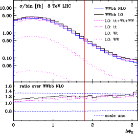
Figure 4: Azimuthal separation of the charged leptons for the $pp\to e^{+}\nu_{e}\mu^{-}\bar{\nu}_{\mu}b\bar{b}+X$ process in the 4F scheme, with the Higgs measurement cuts, apart from the cut on the charged lepton invariant mass $|\Delta\phi_{ll}|<1.8$.

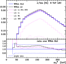
Figure 5: Higgs transverse mass for the $pp\to e^{+}\nu_{e}\mu^{-}\bar{\nu}_{\mu}b\bar{b}+X$ process in the 4F scheme, with the Higgs measurement cuts.

In Figs. 3-5 we show the invariant mass of the two charged leptons ($m_{ll}$), the azimuthal separation of the two leptons ($\Delta\phi_{ll}$) and the transverse mass of the Higgs boson ($m_{T}^{H}$), respectively. The latter is defined as $m_{T}^{H}=\sqrt{(E_{T}^{ll}+E_{T}^{\textrm{miss}})^{2}-|\mathbf{p}_{T}^{ll}+\mathbf{E}_{T}^{\textrm{miss}}|^{2}}$, where $E_{T}^{ll}=\sqrt{|\mathbf{p}_{T}^{ll}|^{2}+m_{ll}^{2}}$. The $m_{ll}$ and $\Delta\phi_{ll}$ variables are used to define the “Higgs topology” cuts, while the $m_{T}^{H}$ distribution is used to extract the Higgs signal in the cut-based analysis by ATLAS ATL (2013). In the plots, results for the full $pp\to e^{+}\nu_{e}\mu^{-}\bar{\nu}_{\mu}b\bar{b}+X$ process at LO (labelled “WWbb LO”) and NLO (“WWbb NLO”) are presented. Also shown are the separate LO calculations for top pair production (“LO: tt”), $W$-boson associated single top production (“LO: Wt”), $b$-quark associated $ll\nu\nu$ production (“LO: WW”) and their sum (“LO: tt+Wt+WW”). These latter processes are defined in the narrow width approximation, i.e. in the LO: tt process we take only diagrams with two s-channel top quark propagators into account (e.g. Fig. 1(a)), LO: Wt has only diagrams with one s-channel top quark propagator (e.g. Fig. 1(b)), while the LO: WW process has no s-channel top quark propagators in any of its contributing diagrams (e.g. Fig. 1(c)); all other parameters are the same as used for the WWbb LO predictions. The differences between the LO: tt+Wt+WW and WWbb LO results stem only from interference effects (among the three contributions to the LO: tt+Wt+WW prediction) which are only included in the complete WWbb simulations. For the $m_{ll}$ and $\Delta\phi_{ll}$ plots, the Higgs topology cut on that distribution is not applied, and is denoted by the vertical line. In the lower inset of the plots, the ratio is taken w.r.t. the WWbb NLO result. Also shown here is the relative scale uncertainty on the NLO result. For the observables studied here, LO scale uncertainties are marginally larger than the NLO scale uncertainties. We refrain from showing these, because scale uncertainties at LO are not a proper estimate of missing higher order corrections, in particular when jet veto’s are applied or when studing exclusive jet bins, as is done here.

As can be seen from the plots, the NLO corrections are small and negative (about -20%) when all the cuts are applied. This is within the NLO scale uncertainty, which is about ${+30}\%\,\,{-20}\%$. It is no surprise that the scale dependence at NLO is still sizeable because the observables considered are rather exclusive; particularly due to the veto of any jets beyond the hardest. There is a visible difference in shape between the LO and NLO results, even though it stays within the NLO scale uncertainties. This difference in shape in the $m_{ll}$ distribution is of particular importance, because the region at large invariant mass, $m_{ll}>80\,\textrm{GeV}$, is used as a background control sample in the ATLAS analysis.

When summing the separate LO calculations for $t\bar{t}$, $Wt$ and $b$-quark included $WW$ production, the final result is very close to the WWbb LO prediction. The bulk is given by top pair production, $Wt$ being about a factor 5 smaller and the contribution from $b$-quark associated $WW$ production is approximately 2 orders of magnitude smaller than top pair production. Interesting to see is that the sum of the separate calculations lies in between the LO and NLO WWbb results. This is not only the case for the 3 observables presented here, but seems to be a general feature of this process. Most likely, this is due to positive interference effects between $t\bar{t}$ and $Wt$ production, which results in a slightly higher cross section when these effects are taken into account. On top of that, the NLO corrections bring the results down again, slightly below the LO result without interference effects.

To conclude, we have presented a calculation of the top quark induced backgrounds to the $H\to WW^{(*)}\to ll\nu\nu$ measurement in the 1-jet bin by computing the NLO corrections to the process $pp\to e^{+}\nu_{e}\mu^{-}\bar{\nu}_{\mu}b\bar{b}+X$ in the four-flavour scheme. This process yields a consistent description of top pair production, $W$-boson associated single top production and $b$-quark associated $WW$ production, including all interference and off-shell effects. Using $H_{T}/2$ as a central renormalisation and factorisation scale, the NLO corrections are small and negative in the Higgs signal region and its uncertainties from renormalisation and factorisation scale dependence are about ${+30}\%\,\,{-20}\%$. There is, however, a difference in shape between LO and NLO in the $m_{ll}$ distribution: the negative NLO corrections at small $m_{ll}$ (Higgs signal region) turn positive for large $m_{ll}$, which is the background control region. Therefore, this might have an effect on the recent Higgs boson measurements and on future high-precision extractions of its coupling constants. Using separate calculations for $t\bar{t}$ and $Wt$ (and $b$-quark associated $WW$) production based on the narrow width approximation for the top quark, yields a fair approximation of the final results, within left-over theoretical uncertainties.

For a more exclusive description of the final state, matching to the parton shower would be required. This would allow for an improved description of the jets, in particular when b-tagging would be applied, and a fair comparison to the data can be made. When matching to the parton shower using the MC@NLO technique Frixione and Webber (2002), care has to be taken to prevent double counting from the NLO corrections and parton shower (non-)emissions from the intermediate top quarks. Work in this direction has already been started.

I would like to thank V. Hirschi for writing the virt_reweighter.py code that has been used to obtain and check some parts of the results presented here. I also thank S. Frixione, F. Maltoni, V. Hirschi, O. Mattelaer, M. Zaro and P. Torrielli for proof-reading this manuscript.

References

- Aad et al. (2012) G. Aad et al. (ATLAS Collaboration), Phys.Lett. B716, 1 (2012), eprint 1207.7214.
- Chatrchyan et al. (2012a) S. Chatrchyan et al. (CMS Collaboration), Phys.Lett. B716, 30 (2012a), eprint 1207.7235.
- Chatrchyan et al. (2012b) S. Chatrchyan et al. (CMS Collaboration), Phys.Lett. B710, 91 (2012b), eprint 1202.1489.
- ATL (2013) Tech. Rep. ATLAS-CONF-2013-030, CERN, Geneva (2013).
- Denner et al. (2011) A. Denner, S. Dittmaier, S. Kallweit, and S. Pozzorini, Phys.Rev.Lett. 106, 052001 (2011), eprint 1012.3975.
- Bevilacqua et al. (2011) G. Bevilacqua, M. Czakon, A. van Hameren, C. G. Papadopoulos, and M. Worek, JHEP 1102, 083 (2011), eprint 1012.4230.
- Denner et al. (2012) A. Denner, S. Dittmaier, S. Kallweit, and S. Pozzorini, JHEP 1210, 110 (2012), eprint 1207.5018.
- Frederix et al. (2013) R. Frederix, S. Frixione, V. Hirschi, F. Maltoni, O. Mattelaer, T. Stelzer, P. Torrielli, and M. Zaro, in preparation.
- Alwall et al. (2011) J. Alwall, M. Herquet, F. Maltoni, O. Mattelaer, and T. Stelzer, JHEP 1106, 128 (2011), eprint 1106.0522.
- Hirschi et al. (2011) V. Hirschi, R. Frederix, S. Frixione, M. V. Garzelli, F. Maltoni, and R. Pittau, JHEP 05, 044 (2011), eprint 1103.0621.
- Ossola et al. (2007) G. Ossola, C. G. Papadopoulos, and R. Pittau, Nucl. Phys. B763, 147 (2007), eprint hep-ph/0609007.
- Ossola et al. (2008) G. Ossola, C. G. Papadopoulos, and R. Pittau, JHEP 03, 042 (2008), eprint 0711.3596.
- Cascioli et al. (2012) F. Cascioli, P. Maierhofer, and S. Pozzorini, Phys. Rev. Lett. 108, 111601 (2012), eprint 1111.5206.
- Frederix et al. (2009) R. Frederix, S. Frixione, F. Maltoni, and T. Stelzer, JHEP 10, 003 (2009), eprint 0908.4272.
- Frixione et al. (1996) S. Frixione, Z. Kunszt, and A. Signer, Nucl. Phys. B467, 399 (1996), eprint hep-ph/9512328.
- Denner et al. (1999) A. Denner, S. Dittmaier, M. Roth, and D. Wackeroth, Nucl.Phys. B560, 33 (1999), eprint hep-ph/9904472.
- Denner et al. (2005) A. Denner, S. Dittmaier, M. Roth, and L. H. Wieders, Nucl. Phys. B724, 247 (2005), eprint hep-ph/0505042.
- Buarque Franzosi et al. (2013) D. Buarque Franzosi, V. Hirschi, and O. Mattelaer, in preparation.
- Papanastasiou et al. (2013) A. Papanastasiou, R. Frederix, S. Frixione, V. Hirschi, and F. Maltoni, Phys.Lett. B726, 223 (2013), eprint 1305.7088.
- Martin et al. (2009) A. Martin, W. Stirling, R. Thorne, and G. Watt, Eur.Phys.J. C63, 189 (2009), eprint 0901.0002.
- Cacciari et al. (2008) M. Cacciari, G. P. Salam, and G. Soyez, JHEP 0804, 063 (2008), eprint 0802.1189.
- Frederix et al. (2012) R. Frederix, S. Frixione, V. Hirschi, F. Maltoni, R. Pittau, and P. Torrielli, JHEP 1202, 099 (2012), eprint 1110.4738.
- Frixione and Webber (2002) S. Frixione and B. R. Webber, JHEP 06, 029 (2002), eprint hep-ph/0204244.