Numerical study of impeller-driven von Kármán flows via a volume penalization method

Abstract

The von Kármán flow apparatus produces a highly turbulent flow inside a cylinder vessel driven by two counter-rotating impellers. Over more than two decades, this experiment has become a very classic turbulence tool, studied for a wide range of physical systems by many groups, with incompressible flow, compressible flow, for magnetohydrodynamics and dynamo studies inside liquid metal, for particle tracking purposes, and recently with turbulent super-fluid helium. We present a direct numerical simulation (DNS) version the von Kármán flow, forced by two rotating impellers. The cylinder geometry and the rotating objects are modelled via a penalization method and implemented in a massive parallel pseudo-spectral Navier-Stokes solver. We choose a special configuration (TM28) of the impellers to be able to compare with set of water experiments well documented. But our good comparison results implied, that our numerical modelling could also be applied to many physical systems and configurations driven by the von Kármán flow. The decomposition into poloidal, toroidal components and the mean velocity fields from our simulations are in agreement with experimental results. We analyzed also the flow structure close to the impeller blades and found different vortex topologies.

Volume penalization Pseudospectral method Moving boundaries von Kármán flow

1 Introduction

A von Kármán experiment is a cylindrical vessel in which a flow is generated by the rotation of two impellers at the extremities of the vessel [1]. Studying turbulence by means of von Kármán fluid experiments has a strong tradition in last two decade. Several teams set up such experiments with different designs in incompressible [2, 3] and compressible flows [4, 5, 6, 7]. This type of experiments was also one of the first setups used to study Lagrangian statistics of turbulent flows [8, 9, 10, 11], by tracking solid particles or bubbles. Recently, a helium super-fluid experiment has been built with the classic von Kármán configuration [12] to reach even higher Reynold number, and to study the interaction of the super and classic fluid.

In the last decade, in order to gain a better understanding of the underlying processes of magnetohydrodynamic and dynamo effect, many experimental groups have investigated experiments using liquid sodium [13, 14, 15, 16]. A very successful experiment used the von Kármán apparatus with Sodium liquid (VKS) hosted in Cadarache which was able to reproduce dynamo action in a turbulent flow [17, 18, 19, 20, 21, 22]. Before starting with sodium experiments, prototypes filled with water were set up, which are smaller than the final VKS machine by a factor of two. They compared and optimized different impeller designs to seek the highest kinematic dynamo growth rate [23, 24].

In this paper we will focus on the purely hydrodynamic properties of the von Kármán flow driven by rotating impellers and keep the investigation of the magnetized dynamics, or other experimental application as a future goal.

In this work we perform direct numerical simulations of a VKS flow, thus a three-dimensional impeller-driven turbulent flow in cylindrical geometry. The geometry of rotating impellers assembled of several basic geometric objects is modeled via an immersed boundary technique (IBM) and implemented in a massive parallel pseudo-spectral Navier-Stokes solver. High resolution simulations allow for the development of a fully developed turbulent flow. We first compare our numerical results with the water campaigns of the Saclay group [25, 26, 27, 28, 29] to validate our numerical modelization approach. We will also study the flow dynamics in the vicinity of impellers, a region not easily accessible experimentally.

2 Numerical method

2.1 Basic equations

We consider the incompressible Navier-Stokes equation

$$\frac{\partial\mathbf{u}}{\partial t}+(\mathbf{u}\cdot\nabla)\mathbf{u}=-\nabla p+\nu\Delta\mathbf{u}$$ (1)

with the velocity field $\mathbf{u}(\mathbf{x},t)$, pressure $p$, viscosity $\nu$. The velocity field additionally fulfills the incompressibility condition $\nabla\cdot\mathbf{u}=0$. At the boundaries we impose a no-slip condition such that the velocity of the fluid equals the velocity of the boundary itself $\mathbf{u}|_{boundary}=\mathbf{V}_{penalized}$. It is zero on the fixed outer cylinder and equals the solid rotation velocity on the disks and the blade structures. The cylindrical wall and the moving impellers are implemented by a penalization method (see 2.3).

2.2 The Fourier-spectral scheme

To solve the equation system a standard pseudo-spectral method is applied using the $\nicefrac{{2}}{{3}}$ rule for dealiasing and resolutions of $256^{3}$ and $512^{3}$ grid points. The time derivative on the left-hand side of the Navier-Stokes equation is discretized via a strongly stable third order Runge-Kutta method [30]. Incompressible turbulent flows have been intensively studied in a periodic box, a classical mathematical framework for theories [31] as well as for numerical simulations of isotropic and homogeneous turbulence [32, 33]. In this geometry the pseudo-spectral numerical method is the most precise global numerical method for a fixed mesh size and the success of this method is essentially due to the efficiency of the Fast Fourier Transform. In the present work, we are using an immersed boundary method to impose no-slip boundary conditions inside the simulation domain. In this framework we lose the spectral precision near the boundaries, but we are able to design any geometry of static or moving structure while keeping the usability of a pseudo-spectral code. The implementation of the penalization boundaries and the moving impellers increase the CPU time by $2$ times. The most time-consuming part of this implementation is the recalculation of the moving boundaries in each step. For future MHD simulations we expect a factor below $2$, as the penalization then comsumes less time compared to the solution of the basic equations. Those methods are sufficiently accurate to reproduce standard benchmarks [34] and benchmarks depending crucially on the boundary layer solution [35]. The used method will now be explained in more detail.

2.3 Penalization method

To simulate flows within a solid cylindrical boundary and moving impellers with complex shape, a penalization method is applied. For points inside the boundaries a “pseudo” forcing term is added to the right-hand side of the Navier-Stokes equation (1), which adjusts the velocity exactly to the prescribed value in and on the wall or the impellers. The method we used to calculate the force, which is first introduced in [36, 37], is called direct forcing and allows to calculate the force directly from the Navier-Stokes equation without the necessity of further auxiliary parameters. To increase the precision of the boundary layers, we used a predictor for the pressure gradient [38].

As we deal with complex geometries the boundaries of the objects do not coincide with the rectangular grid. This makes it necessary to interpolate at the boundary, for which we take the volume fraction $V_{b}$ occupied by the solid object into account. Regarding the volume of each cell $V_{c}=n^{3}\Delta x\Delta y\Delta z$, the force is weighted with the factor $\nicefrac{{V_{b}}}{{V_{c}}}$. Practically, this is performed via a Monte-Carlo method using 50 random points within each cell to calculate the volume [37]. The details of this penalization method were described and tested in another fluid context [35].

The solid rotating velocity of the impellers is simply given by the angular velocity $\mathbf{\Omega}$ and the distance from the axis $\mathbf{r}$ as $\mathbf{V}_{boundary}=\mathbf{\Omega}\times\mathbf{r}$. The angular velocity of the impellers can be set independently for each impeller.

2.4 Configurations of our numerical experiments

2.4.1 Numerical experiment setup

Our aim is to model a configuration similar to the von Kármán experiments in which a cylindrical vessel is filled with liquid. The fluid is driven by two counter-rotating impellers, one on each side of the vessel. Each impeller consists of a disk on which several blades are mounted.

We create an embedded cylinder inside the periodic box, using our penalization method, with a radius $R_{c}=3.0$. Though the periodicity is kept along the z axis to decrease Gibbs oscillations, the velocity at the end of the cylinder is close to zero due to the symmetry of the system. The height of the cylinder is $2\pi$, giving an aspect ratio of $2\pi/R_{c}$. In experimental setups this height varies from 2 up to 3 cylinder radii. The interior of this cylinder represents $\sim 71\%$ of the total computing domain.

For one set of simulations we choose a very similar configuration of the curved disk-blades to the setup called “TM28” [23] with a distance between the disks of $1.8R_{c}$, a radius of the rotating disk of $R_{d}=0.9R_{c}$, a height of the eight blades of $0.2R_{c}$ and a curvature radius of the blades of $C=0.5R_{c}$. The angle of the expelled flow at the end of the blades is given by $\alpha=\mbox{arcsin}\left(\nicefrac{{R_{d}}}{{2C}}\right)\approx 1.11976~{}rad\sim 64.15~{}deg$. The simulated straight blade configuration is close to the “TM70” and “TM80” configuration [26, 28, 24], with eight blades per disk. A difference is that our disk radius is $R_{d}=0.9R_{c}$ instead of ($R_{TM70}=0.75R_{c}$, $R_{TM80}=0.95R_{c}$). We call this configuration straight configuration. Here, $C=\pm\infty$ and $\alpha=0$.

In the following we analyze these two blade geometries (TM28 curved and straight blades). The disks are always counter-rotating with the same rotation rate. Depending on the rotation direction we have two different blade curvatures (called $+$ or $-$) (see figure 1).

Figure 1: Simulated impellers with 8 curved blades (left) and 8 straight blades (right): A positive curvature, denoted (+), means that the convex side of the blade points in the turning direction of the impeller, while for a negative value, denoted (-), it is the concave side.

2.4.2 Non dimensional numbers

We have chosen six simulations to highlight our results. We vary the viscosity $\nu$ controlling the dissipative term, the rotation rate $\Omega$ of the impellers, and the curvature of the blades. Of course other parameters such as the geometry of the blade, the number of blades, the difference in the rotation rate of the disks might change the topology of the flow and the quantitative results.

From our numerical data we compute a set of meaningful non-dimensional numbers (see table 1). The Reynolds number accessible with direct numerical simulations with $512^{3}$ grid points is as usual a few orders of magnitude lower than experimental Reynolds numbers. Nevertheless, at this Reynolds number the flow is turbulent. Our measured fluctuation level $\delta=\nicefrac{{\overline{\langle\mathbf{u}^{2}\rangle}}}{{\langle\overline{\mathbf{u}}^{2}\rangle}}$ defined in [39] is similar to that obtained from the water experiments for synchronized rotating disks and with an annulus deviator configuration in the “TM60” and “TM73” setup. With asynchronous disk rotations or without annulus, this level of fluctuation could be higher (above $2.0$) [39].

The efficiency $E_{f}=\nicefrac{{U_{max}}}{{\Omega R_{d}}}$ of the impellers, which measures how much energy is injected into the fluid, is defined as the maximum velocity of the fluid in the bulk induced by the impeller motion. The variation of the $E_{f}$ as a function of the expelled flow angle $\alpha$ for different experimental configurations is confronted with our numerics in figure 4.b. With a Reynolds number three orders of magnitude lower than the experiments, we nevertheless have a good agreement with the experimental efficiency. The efficiency number decreases with the same slope found in the water experiments. We noticed that our straight blade efficiency is almost identical with the “TM70” configuration efficiency. For the positive curved blades our numerical data is closer to the “TM60” configuration (16 blades) than to the “TM28” (8 blades).

The ratio of the root mean square velocity and the maximum velocity of the impellers ($U_{rms}/V_{max}$) is pretty close to the TM28 experiment for our higher rotation rate simulation ($1.6\Omega=2.4$).

Another non-dimensional number is the ratio of rotation period of the impellers $T_{\Omega}=1/f=\frac{2\pi}{\Omega}$ and the large eddy turn over time $T_{nl}$. Our simulations are in the same disk rotation regime as the experiments (see the last line of table 1) showing that there is a bit more than two large eddy turn over times during one turn of the impellers.

	TM28	curved (+)	curved (-)	(straight)	(+) 512	(+) $1.6\Omega$	(+) $\nu/2$
grid size	—	$256^{3}$	$256^{3}$	$256^{3}$	$512^{3}$	$512^{3}$	$512^{3}$
$\nu$	$10^{-6}~{}m^{2}/s$	$0.005$	$0.005$	$0.005$	$0.005$	$0.005$	$0.0025$
$\Omega$	$28.4628s^{-1}$	$1.5$	$1.5$	$1.5$	$1.5$	$2.4$	$1.5$
$U_{rms}$	$1~{}m/s$	$0.9397$	$1.0641$	$1.0843$	$0.9429$	$1.5352$	$0.9619$
$U_{max}$		$2.268$	$3.143$	$2.859$	$2.268$	$3.616$	$2.268$
$L$	$0.1$ m	$1.6831$	$1.9011$	$1.9149$	$1.6349$	$1.9277$	$1.9038$
$T_{nl}$	$0.1$ s	$1.7911$	$1.7865$	$1.7660$	$1.7339$	$1.2556$	$1.9792$
$R_{exp}$	$2.84~{}10^{5}$	$2430$	$2430$	$2430$	$2430$	$3888$	$4860$
$R_{num}$	$10^{5}$	$316$	$404$	$415$	$308$	$591$	$732$
$E_{f}$	$0.64$	$0.50$	$0.698$	$0.635$	$0.504$	$0.502$	$0.504$
$\delta$	$1.5-2.2$	$1.452$	$1.433$	$1.487$	$1.40$	$1.519$	$1.519$
$U_{rms}/V_{max}$	$0.40$	$0.232$	$0.262$	$0.267$	$0.232$	$0.379$	$0.237$
$\nicefrac{{T_{\Omega}}}{{T_{nl}}}$	$2.207$	$2.34$	$2.338$	$2.3446$	$2.371$	$2.0850$	$2.1164$

Table 1: Simulation quantities are compared with water experiments results from [23, 26, 39] and specially the configuration “TM28”. We collected and defined several quantities or non-dimensional numbers: $\nu$ the kinematic viscosity of water or in our simulations, $\Omega$ the rotation rate, $U_{rms}=\overline{\sqrt{2E(t)}}$, $U_{max}$ is the (spatial) maximum of the (time-averaged) mean velocity field in the bulk in the range $-0.8R_{c}<z<0.8R_{c}$, where z=0 is the center of the cylinder. $L=\frac{2\pi}{\sum E(k)}\sum E(k)/k$ is the integral length scale computed with $E(K)$, the isotropic spectral density of the kinetic energy, and $T_{nl}=L/U_{rms}$ is the eddy turn over time. We used the experimental Reynolds number definition of VKE-VKS experiments $R_{exp}=\nicefrac{{\Omega R_{d}R_{c}}}{{\nu}}$. To compare with numerical works, we define another Reynolds number $R_{num}=\nicefrac{{U_{rms}L}}{{\nu}}$. The efficiency $E_{f}=\nicefrac{{U_{max}}}{{\Omega R_{c}}}$ of the impellers states how much energy is injected into the fluid. $\delta=\nicefrac{{\overline{\langle\mathbf{u}^{2}\rangle}}}{{\langle\overline{\mathbf{u}}^{2}\rangle}}$ is the fluctuation level defined in [39]. We present also the ratios $U_{rms}/V_{max}$ and $T_{\Omega}/T_{nl}=\frac{2\pi U_{rms}}{\Omega L}$. Our simulations are during more than $20T_{\Omega}$ (turns of the impellers), which is the duration of the time average computation.

3 Mean bulk flow structure

3.1 Global flow profiles

While integrating the Navier-Stokes equations we additionally time averaged the velocity field. The stream lines and the vector field of the mean flow $\overline{\mathbf{u}}$ are shown in figure 2.a and figure 2.b, respectively. These images reproduce the classical images of a S2T2 flow of the von Kármán flow. For comparison, a snapshot of the enstrophy (figure 2.c) shows interacting vortex filaments in the bulk region which is characteristic to a turbulent flow. The vorticity is produced and thus very high near the blades. This observation will be analyzed in detail in section 4.

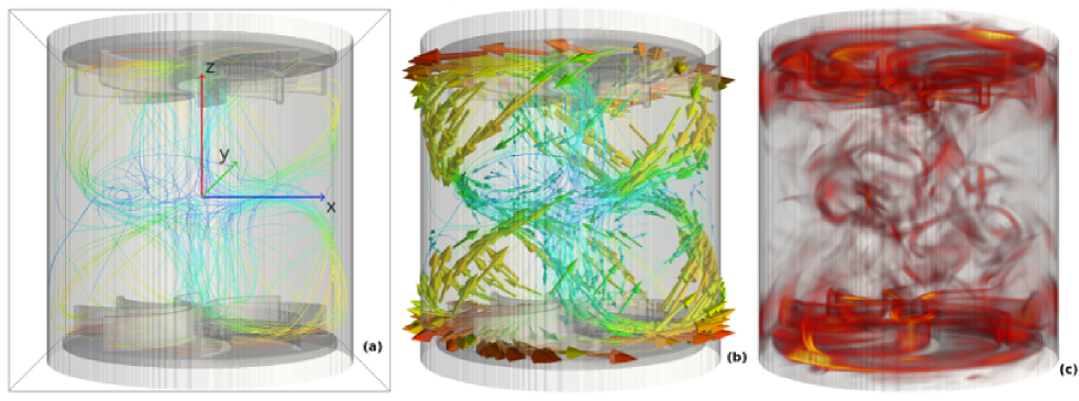
Figure 2: (a) Streamlines and (b) vector field of the time-averaged flow and (c) a snapshot of the vorticity with (+) configuration.

3.2 Poloidal and toroidal components

For further analysis of the simulated flows we performed a decomposition into poloidal and toroidal components of the form

$$\mathbf{u} =\mathbf{u}_{tor}+\mathbf{u}_{pol} =\nabla\times[\Psi(r,\theta,z)\mathbf{e}_{z}]+\nabla\times\nabla\times[\Phi(r,\theta,z)\mathbf{e}_{z}]$$ (2)

with unique potential functions $\Psi$ and $\Phi$ and the unit vector in $z$ direction $\mathbf{e}_{z}$. To be precise, in the periodic box, we normally need to add a component $F(z)$ depending only on $z$ (see [40] and (course 2, C. A Jones) [41]). Although our penalized cylinder is periodic along the z axis there is no mean flow crossing the box as the gap between the cylinder and the disks is small. We checked that $F$ is zero (up to the numerical digit precision).

This decomposition has also been performed with the experimental data with the TM28 impellers, which allows a comparison of experimental and simulated data. Supposing axial symmetry around the z axis, we can compute the poloidal and toroidal two dimensional fields $\nabla\times[\Psi(r,z)\mathbf{e}_{z}]$ respectively $\nabla\times\nabla\times[\Phi(r,z)\mathbf{e}_{z}]$ (see figure 3) and compare them to figure 3 of [23]. We have visually a good agreement, the poloidal flow consists of two large scale vortices in the regions $z<0$ and $z>0$, where the toroidal components respectively point in opposite directions. Impellers with different curvature (negative curvature and straight blades) produce the same kind of flow structure. From the images it is difficult to distinguish between the different blades configurations. We therefore present in table 2 the mean and maximum velocity of the poloidal/toroidal components, all of them rescaled by their respective maximum velocity of the impellers $V_{max}=\Omega R_{d}$.

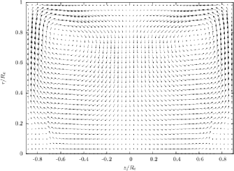
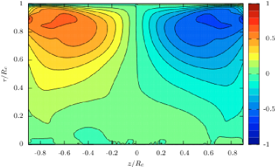
Figure 3: Projections of the poloidal (left) and toroidal (right) components generated by impellers with curved blades and positive direction.

	TM28	(+)	(-)	(straight)	(+) 512	(+) $1.6\Omega$	(+) $\nu/2$
$u_{pol,mean}$	0.199	0.174	0.141	0.164	0.184	0.166	0.179
$u_{pol,max}$	0.492	0.425	0.380	0.453	0.443	0.452	0.460
$u_{tor,mean}$	0.281	0.205	0.228	0.245	0.217	0.202	0.217
$u_{tor,max}$	0.691	0.535	0.824	0.708	0.538	0.530	0.509
$\Gamma_{mean}$	0.71	0.850	0.621	0.670	0.847	0.822	0.825
$\Gamma_{max}$	0.71	0.794	0.461	0.640	0.824	0.854	0.904
$T$	-	1.000	1.295	1.375	-	-	-

Table 2: Quantities from experiments and simulations : the maximum and the mean of the poloidal and toroidal velocity and the respective ratio $\Gamma_{max}=\nicefrac{{u_{pol,max}}}{{u_{tor,max}}}$ and $\Gamma_{mean}=\nicefrac{{u_{pol,mean}}}{{u_{tor,mean}}}$. All the velocities are normalized by the maximum velocity of the impellers $V_{max}=\Omega R_{d}$. A quantification of the poloidal and toroidal components is done by extracting the maximum and mean values in the bulk, the region $-0.8R_{c}<z<0.8R_{c}$. In addition, the average torque $T$ on the impellers has been computed for the three simulations with lower resolution and normalized to the value obtained in the run (+).

Those values can be compared to the experimental ones [23]. Our velocities of the $(+)$ configuration are $10\%-20\%$ lower than the experimental data of “TM28”. This could be explained by the fact that our efficiency coefficient is lower than the “TM28” configuration (see figure 4 right), implying a smaller velocity in the central region of the vessel. We also compare the ratio of the poloidal over the toroidal velocity versus the expulsion angle of the blades $\alpha$ with different water experiment results [24, 28, 23]. This ratio was used to seek the dynamo onset as a control parameter. Like the efficiency the ratio $\Gamma_{mean}$ for the $(+)$ configuration is closer to the “TM60” than the “TM28” setup (figure 4 left). However we stress that our ratios have also a positive slope. Even if there is not a perfect agreement our ratios are quite close to the different experimental measurements.

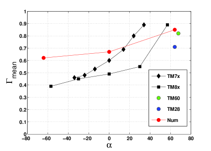
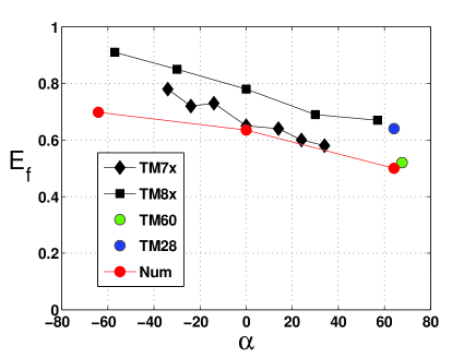
Figure 4: From different water experiment setups given in data tables (TM7x [24], TM8x [28], TM60 and TM28 [23]) and from our numerical results, we plot (left) the ratio of the poloidal and the toroidal mean velocity ($\Gamma_{mean}$) and (right) the efficiency $E_{f}=\nicefrac{{U_{max}}}{{\Omega R_{c}}}$ of the impellers both versus the flow expulsion angle $\alpha$ at the end of the blades.

3.3 Impact of viscosity and rotation speed

In order to study impact of the viscosity and the disk rotation rate on the mean flow structure we performed additional simulations with curved impeller blades and positive turning direction. In the first of these runs we increase the resolution to $512^{3}$ grid points (Run $(+)~{}512$ in table 1&2), while all other parameters are unchanged. This simulation can be seen as a convergence test. The velocities for the toroidal and poloidal component are slightly closer to the experimental values, but the non dimensional quantities, especially the poloidal-toroidal ratios $\Gamma$, are unchanged, showing that at $256^{3}$ grid points, our simulations are already converged.

In the second run (run $(+)~{}1.6\Omega$ in tables 1&2), the angular velocity of the impellers is increased by a factor of 1.6, while all other parameters as well as the resolution are unchanged. The Reynolds number then increases to $Re=3888$. The listed values remain constant, only the ratio of the rotation period over the eddy turn over time slightly decreases.

In the last run the viscosity is lowered by factor 2 (run $(+)~{}\nu/2$ in tables 1&2) and the resolution is increased to $512^{3}$ grid points. In this case the Reynolds number increases up to $Re=4860$. Regarding all quantities obtained in the simulations, there is evidently no major influence of rotation speed and viscosity on the mean flow profile. Only the fluctuation rate $\delta$ slightly increases.

The mean flow quantities which we present do not change with the rotation rate or the viscosity. This implies that the corresponding simulations are already in an asymptotic regime, where the Reynolds number has only little effect on the large scale structure of the flow. Indeed, the range of Reynolds number numerically acheived in our work ($2500-4800$), is at the edge the inertial regime of water experimentals results ([29] see their Fig. 5 and Fig. 7). In this experimental campain, the Reynolds number has been increased progressivelly by growing the rotation frequency of the disks, to explore different phases : viscous, transition and inertial regimes.

4 Local near-blade structures

4.1 Vortex generation behind blades

Besides the general flow structure imposed by the impellers, our main interest lies in the near blade flow in the frame of reference of the rotating impeller. Here, we present and analyze the structures obtained in the three different configurations (($+$), ($-$), straight) with $n=256$. We construct the mean flow in the rotating frame of reference by first averaging the flow each time the blades pass the same positions, which is every eighth of a turning period. As we expect to find the same mean flow at each blade we also take the spatial average for rotations around $90^{\circ}$. As the running time of our simulation corresponds to 20 impeller turns we were able to average over 640 realizations. The mean flow in the rotating frame is obtained from this average by subtracting a solid rotation $\mathbf{u}^{\ast}=\mathbf{u}-\mathbf{\Omega}\times\mathbf{r}$.

To get clear pictures of the flow we consider two different planes: one parallel to the disk plane, with a view from the top and the other perpendicular to the disk (the position of the perpendicular plane is indicated by a red line in the top view (left column of figure 5)). In the top view, we show the velocity projected onto the plane while its amplitude is represented by a color map. This perspective shows how the flow is sucked in from above to the center, moving between the blades and how it is finally expelled from the disk outwards. Just by looking at the left column of figure 5, we can easily distinguish between the different configurations, specially the $(+)$ and the $(-)$, where the expelled flow in the rotating frame has the same rotational direction as the disk rotation. The horizontal component represents the major part of the magnitude of the full velocity along the blade. There is clearly an acceleration from the center to the expulsion area. The most rapid velocity is generally along the pushing blade wall. A small sucking area is located just behind at the end of the blade.

In the perpendicular plane we decide to visualize the velocity by streamlines to highlight the topology of perpendicular flows. Note that the projected velocity is not solenoidal, thus streamlines may have an end point. In all three simulations, (right column of figure 5) the streamline plots show vortex rolls emerging directly behind the moving blade, as vortices are ripped off at the blade’s edge. Those vortices appear to take most of the space between the blades. Clearly, the negative configuration (-) has a different topology than the two others. This observation agrees with the horizontal velocity in the top views. The cut along the red line allows the visualization of the mean flow vortex at different radii for different cells. In the positive configuration (+), it can be deduced that a cone vortex is produced along the pushing blade in each inter-blade cell. Those vortices are also present in the straight configuration which is, however, less clear for the negative configuration $(-)$.

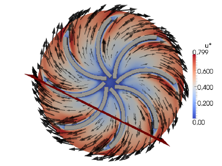
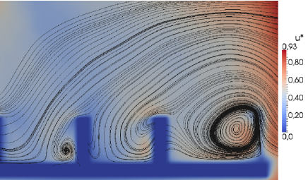
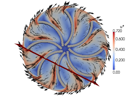
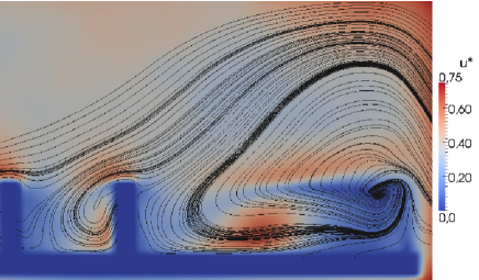
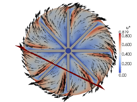
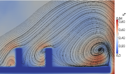
Figure 5: Visualization of the velocity field on a top view (left) and the streamlines of velocity on a transverse view (right), for our three configurations (from top to bottom (+), (-), (straight)). The velocity is averaged in time, projected on the plane, and computed in the rotating frame ($\mathbf{u}^{\ast}=\mathbf{u}-\mathbf{\Omega}\times\mathbf{r}$). In all images, the color map represents the magnitude of the velocity. The transverse view planes are perpendicular to the red line shown on the top view planes. Not all of the perpendicular planes associated with the red lines is plotted (only 70% of the red line of the left side). The position of the blades helps to relate the top and side views. Note that this projection of the velocity in the considered plane is not solenoidal, thus streamlines could end at the boundary, where the projected velocity tends to zero. Streamlines of the 3D flow do not enter in the solid object, but instead slide along the boundary. This behaviour is not captured by the 2D projection.

5 Discussions and perspectives

5.1 Numerical and experimental comparisons

By means of direct numerical simulations using a penalization technique we are able to reproduce the large scale structure of experimental von Kármán flows produced by moving impellers. Our good agreement with the experimental results could be explained by the fact that the mean flow geometry and other global quantities are converging rapidly even at low Reynolds number.

The natural next step could be to seek the small scale properties of the von Kármán flow, like the studies on filaments [3, 42], effect of large scales on small scales [7] or the energy injection [43, 44]. Of course, direct numerical studies with confined flows in the full von Kármán geometry remain a challenge asking for a big increase of spatial resolution. Our modelization using the penalization could be easily used to explore different experimental setups - at least for the large scale properties.

5.2 Vortex and Dynamos

We found a characteristic outwards spiraling vortex between the blades. Note that the influence of the vortex generated around the blades is suspected to have a strong impact on the dynamo effect [45]. Some numerical results assuming a dynamo mechanism concentrated around the disk-blade structure [46, 47] have found that the magnetic mode has a dipole structure according to the experimental results. The geometry of the experimental magnetic mode cannot be explained by a mean flow dynamo only. Recent numerical studies using FLUENT ($k-\epsilon$)-RANS simulations [48] computed the $\alpha$-tensor produced by the vortex dynamics, given a switch between $\alpha^{2}$ and $\alpha-\Omega$ dynamo types.

Despite these vortex dynamics, without soft iron impellers the dynamo threshold was not achieved. The material of the impellers plays a crucial role for the efficiency of the dynamo action [49, 50, 51]. The material properties of sodium make in-situ diagnostics very difficult. Direct numerical simulations provide a unique tool to assess spatially and temporally resolved variables. With our dynamics of the blade vortex and correct treatment of the magnetic properties of the solid impellers, all the physical ingredients should be present to address those different questions, to seek the interaction between the conducting fluid and the ferromagnetic impellers. We could also check the different dynamo onset prediction or measurement of the different configurations produce by the variation of the blade geometries or material properties [51].

5.3 Long term dynamics

When the water experiments are running during a long time, the von Kármán mean flow can change to different topology solutions, breaking symmetries [27, 29, 52]. In the experiment, the typical time scale to record this multi-stability is around $10^{5}$ to $10^{6}$ hydrodynamic large eddy turnover times. In our present simulations, we are completely out of reach to record such dynamics: we computed $20$ disk turns, which represent around $45$ eddy turnover times only. It will thus be very interesting, even if less popular than the highest resolution limit, to perform long numerical runs with moderate grid points to reach and study the long time physical behaviors or to improve statistical data.

6 Acknowledgment

We acknowledge fruitful discussions with Nicolas Plihon, Arnaud Chiffaudel. Parts of this research were supported by Research Unit FOR 1048, project B2, and the French Agence Nationale de la Recherche under grant ANR-11-BLAN-045, projet SiCoMHD. Access to the IBM BlueGene/P computer JUGENE at the FZ Jülich was made available through the project HBO36. Computer time was also provided by GENCI in the IDRIS facilities and the Mesocentre SIGAMM machine, hosted by the Observatoire de la Côte d’Azur.

References

- [1] T. von Kármán. Uber laminare und turbulente reibung. Z . Angew. Math. Mech., 1:233, 1921.
- [2] D. Dijkstra and G. J. F. Van Heijst. The flow between two finite rotating disks enclosed by a cylinder. Journal of Fluid Mechanics, 128:123–154, 1983.
- [3] S. Douady, Y. Couder, and M. E. Brachet. Direct observation of the intermittency of intense vorticity filaments in turbulence. Physical Review Letters, 67(8):983–986, August 1991.
- [4] S. Fauve, C. Laroche, and B. Castaing. Pressure fluctuations in swirling turbulent flows. Journal de Physique II, 3(3):271–278, mar 1993.
- [5] R. Labbé J.-F. Pinton. Correction to taylor hypothesis in swirling flows. Journal de Physique II (France), 4:1461–1468, 1994.
- [6] P. Abry, S. Fauve, P. Flandrin, and C. Laroche. Analysis of pressure fluctuations in swirling turbulent flows. Journal de Physique II, 4(5):725–733, May 1994.
- [7] R. Labbé, J.-F. Pinton, and S. Fauve. Study of the von kármán flow between coaxial corotating disks. Physics of Fluids, 8(4):914–922, April 1996.
- [8] N. Mordant, P. Metz, O. Michel, and J.-F. Pinton. Measurement of lagrangian velocity in fully developed turbulence. Physical Review Letters, 87(21):214501, November 2001.
- [9] N. Mordant, J. Delour, E. Léveque, A. Arnéodo, and J.-F. Pinton. Long time correlations in lagrangian dynamics: A key to intermittency in turbulence. Physical Review Letters, 89(25):254502, December 2002.
- [10] A. La Porta, Greg A. Voth, F. Moisy, and Eberhard Bodenschatz. Using cavitation to measure statistics of low-pressure events in large-reynolds-number turbulence. Physics of Fluids, 12(6):1485–1496, June 2000.
- [11] A. La Porta, Greg A. Voth, Alice M. Crawford, Jim Alexander, and Eberhard Bodenschatz. Fluid particle accelerations in fully developed turbulence. Nature, 409(6823):1017–1019, February 2001.
- [12] B. Saint-Michel, E. Herbert, J. Salort, C. Baudet, M. Bon Mardion, P. Bonnay, M. Bourgoin, B. Castaing, L. Chevillard, F. Daviaud, P. Diribarne, B. Dubrulle, Y. Gagne, M. Gibert, A. Girard, B. Hébral, Th. Lehner, and B. Rousset. Probing quantum and classical turbulence analogy through global bifurcations in a von karman liquid helium experiment. submit, 2013.
- [13] A. Gailitis, O. Lielausis, S. Dement’ev, E. Platacis, A. Cifersons, G. Gerbeth, T. Gundrum, F. Stefani M. Christen, H. Hanel, and G. Will. Detection of a flow induced magnetic field eigenmode in the riga dynamo facility. Phys. Rev. Lett., 84:4365, 2000.
- [14] A. Gailitis, O. Lielausis, S. Dement’ev, A. Cifersons, G. Gerbeth, T. Gundrum, F. Stefani M. Christen, H. Hanel, and G. Will. Magnetic field saturation in the riga dynamo experiment. Phys. Rev. Lett., 86:3024, 2001.
- [15] U. Müller and R. Stieglitz. Can the earth’s magnetic field be simulated in the laboratory? Naturwissenschaften, 87:381, 2000.
- [16] R. Stieglitz and U. Müller. Experimental demonstration of a homogeneous two-scale dynamo. Phys. Fluids, 13:561, 2001.
- [17] R. Monchaux, M. Berhanu, M. Bourgoin, M. Moulin, Ph. Odier, J.-F. Pinton, R. Volk, S. Fauve, N. Mordant, F. Pétrélis, A. Chiffaudel, F. Daviaud, B. Dubrulle, C. Gasquet, L. Marié, and F. Ravelet. Generation of a magnetic field by dynamo action in a turbulent flow of liquid sodium. Phys. Rev. Lett., 98:044502, 2007.
- [18] M. Berhanu, R. Monchaux, S. Fauve, N. Mordant, F. Pétrélis, A. Chiffaudel, F. Daviaud, F. Ravelet, M. Bourgoin, Ph. Odier, J.-F. Pinton, R. Volk, B. Dubrulle, and L. Marié. Magnetic field reversals in an experimental turbulent dynamo. Europhys. Lett., 77:59001, 2007.
- [19] Romain Monchaux, Michael Berhanu, Sebastien Aumaitre, Arnaud Chiffaudel, Francois Daviaud, Berengere Dubrulle, Florent Ravelet, Stephan Fauve, Nicolas Mordant, Francois Petrelis, Mickael Bourgoin, Philippe Odier, Jean-Francois Pinton, Nicolas Plihon, and Romain Volk. The von kármán sodium experiment: Turbulent dynamical dynamos. Physics of Fluids, 21(3):035108–21, March 2009.
- [20] M. Berhanu, B. Gallet, R. Monchaux, M. Bourgoin, Ph. Odier, J.-F. Pinton, N. Plihon, R. Volk, S. Fauve, N. Mordant, F. Pétrélis, S. Aumaître, A. Chiffaudel, F. Daviaud, B. Dubrulle, and F. Ravelet. Bistability between a stationary and an oscillatory dynamo in a turbulent flow of liquid sodium. Journal of Fluid Mechanics, 641:217–226, 2009.
- [21] M. Berhanu, G. Verhille, J. Boisson, B. Gallet, C. Gissinger, S. Fauve, N. Mordant, F. Pétrélis, M. Bourgoin, P. Odier, J.-F. Pinton, N. Plihon, S. Aumaître, A. Chiffaudel, F. Daviaud, B. Dubrulle, and C. Pirat. Dynamo regimes and transitions in the VKS experiment. The European Physical Journal B, 77:459–468, September 2010.
- [22] B. Gallet, S. Aumaître, J. Boisson, F. Daviaud, B. Dubrulle, N. Bonnefoy, M. Bourgoin, Ph. Odier, J.-F. Pinton, N. Plihon, G. Verhille, S. Fauve, and F. Pétrélis. Experimental observation of spatially localized dynamo magnetic fields. Physical Review Letters, 108(14):144501, April 2012.
- [23] L. Marié, J. Burguete, F. Daviaud, and J. Léorat. Numerical study of homogeneous dynamo based on experimental von kármán type flows. The European Physical Journal B - Condensed Matter and Complex Systems, 33(4):469–485, June 2003.
- [24] F. Ravelet, A. Chiffaudel, F. Daviaud, and J. Léorat. Toward an experimental von kármán dynamo: Numerical studies for an optimized design. Physics of Fluids, 17(11):117104, November 2005.
- [25] Louis Marié. Transport de moment cinétique et de champ magnétique par un écoulement tourbillonnaire turbulent: Influence de la Rotation. THESE, Université Paris-Diderot - Paris VII, September 2003.
- [26] L. Marié and F. Daviaud. Experimental measurement of the scale-by-scale momentum transport budget in a turbulent shear flow. Phys. Fluids, 16:457, 2004.
- [27] Florent Ravelet, Louis Marié, Arnaud Chiffaudel, and Fran¸cois Daviaud. Multistability and memory effect in a highly turbulent flow: Experimental evidence for a global bifurcation. Physical Review Letters, 93(16):164501, October 2004.
- [28] Florent Ravelet. Bifurcations globales hydrodynamiques et magnetohydrodynamiques dans un ecoulement de von Karman turbulent. THESE, Ecole Polytechnique X, September 2005.
- [29] F. Ravelet, A. Chiffaudel, and F. Daviaud. Supercritical transition to turbulence in an inertially driven von kármán closed flow. Journal of Fluid Mechanics, 601:339–364, 2008.
- [30] C.-W. Shu and S. Osher. Efficient implementation of essentially non-oscillatory shock-capturing schemes. J. Comp. Phys., 77:439ff, 1988.
- [31] U. Frisch. Turbulence : The Legacy of A.N Kolmogorov. Cambridge University Press, 1996.
- [32] S.A. Orszag and Jr J.S. Patterson. Numerical simulation of three-dimensional homogeneous isotropic turbulence. Phys. Rev. Lett., 28:76–79, 1972.
- [33] A. Vincent and M. Meneguzzi. The spatial structure and the statistical propierties of homegeneous turbulence. J. Fluid Mech., 225:1–25, 1991.
- [34] M. Minguez, R. Pasquetti, and E. Serre. High-order large-eddy simulation of flow over the Ahmed body car model. Physics of Fluids, 20(9):095101–095101–17, September 2008.
- [35] H. Homann, J. Bec, and R. Grauer. Effect of turbulent fluctuations on the drag and lift forces on a towed sphere and its boundary layer. Journal of Fluid Mechanics, 721:155–179, 2013.
- [36] J. Mohd-Yusof. Combined immersed boundary/b-spline methods for simulations of flow in complex geometries. Center for Turbulence Research Annual Research Briefs, pages 317–327, 1997.
- [37] E. A. Fadlun, R. Verzicco, P. Orlandi, and J. Mohd-Yusof. Combined immersed-boundary finite-difference methods for three-dimensional complex flow simulations. J. Comp. Phys., 161:35ff, 2000.
- [38] David L. Brown, Ricardo Cortez, and Michael L. Minion. Accurate projection methods for the incompressible Navier-Stokes equations. Journal of Computational Physics, 168(2):464–499, April 2001.
- [39] Pierre-Philippe Cortet, Pantxo Diribarne, Romain Monchaux, Arnaud Chiffaudel, Fran¸cois Daviaud, and Bérengère Dubrulle. Normalized kinetic energy as a hydrodynamical global quantity for inhomogeneous anisotropic turbulence. Physics of Fluids, 21(2):025104–025104–11, February 2009.
- [40] B. J. Schmitt and W. von Wahl. Decomposition of Solenoidal Fields into Poloidal Fields, Toroidal Fields and the Mean Flow. Applications to the Boussinesq-Equations. Lecture Notes in Math., 1530:291ff, 1992.
- [41] P. Cardin and L.F. Cugliandolo. Dynamos, volume Session LXXXVIII, 2007 of Les Houches - Ecole d’Ete de Physique Theorique. Amsterdam: Elsevier, 2008.
- [42] O. Cadot, S. Douady, and Y. Couder. Characterization of the low pressure filaments in a three-dimensional turbulent shear flow. Physics of Fluids, 7(3):630–646, March 1995.
- [43] N. Mordant, J.-F. Pinton, and F. Chillà. Characterization of turbulence in a closed flow. Journal de Physique II, 7(11):1729–1742, November 1997.
- [44] R. Labbé, J.-F. Pinton, and S. Fauve. Power fluctuations in turbulent swirling flows. Journal de Physique II, 6(7):12, 1996.
- [45] F. Petrelis, N. Mordant, and S. Fauve. On the magnetic fields generated by experimental dynamos. Geophysical & Astrophysical Fluid Dynamics, 101:289–323, June 2007.
- [46] R. Laguerre, C. Nore, A. Ribeiro, J. Léorat, J.-L. Guermond, and F. Plunian. Impact of impellers on the axisymmetric magnetic mode in the vks2 dynamo experiment. Physical Review Letters, 101(10):104501, 2008.
- [47] André Giesecke, Frank Stefani, and Gunter Gerbeth. Role of soft-iron impellers on the mode selection in the von kármán-sodium dynamo experiment. Physical Review Letters, 104(4):044503, January 2010.
- [48] F. Ravelet, B. Dubrulle, F. Daviaud, and P.-A. Ratié. Kinematic tensors and dynamo mechanisms in a von kármán swirling flow. Physical Review Letters, 109(2):024503, July 2012.
- [49] Gautier Verhille, Nicolas Plihon, Mickal Bourgoin, Philippe Odier, and Jean-François Pinton. Induction in a von kármán flow driven by ferromagnetic impellers. New Journal of Physics, 12(3):033006, 2010.
- [50] A Giesecke, C Nore, F Stefani, G Gerbeth, J Léorat, W Herreman, F Luddens, and J-L Guermond. Influence of high-permeability discs in an axisymmetric model of the cadarache dynamo experiment. New Journal of Physics, 14(5):053005, May 2012.
- [51] Sophie Miralles, Nicolas Bonnefoy, Mickael Bourgoin, Philippe Odier, Jean-François Pinton, Nicolas Plihon, Gautier Verhille, Jean Boisson, François Daviaud, and Bérengère Dubrulle. Dynamo threshold detection in the von kármán sodium experiment. Physical Review E, 88(1):013002, July 2013.
- [52] A. de la Torre and J. Burguete. Slow dynamics in a turbulent von kármán swirling flow. Physical Review Letters, 99(5):054101–4, 2007.