UFIFT-HEP-10-

On Type 0 Open String Amplitudes and the Tensionless Limit
Francisco Rojas 

Instituto de Física Teórica, UNESP-Universidade Estadual Paulista

R. Dr. Bento T. Ferraz 271, Bl. II, São Paulo 01140-070, SP, Brasil

The sum over planar multi-loop diagrams in the NS+ sector of type 0 open strings in flat spacetime has been proposed by Thorn as a candidate to resolve non-perturbative issues of gauge theories in the large $N$ limit. With $SU(N)$ Chan-Paton factors, the sum over planar open string multi-loop diagrams describes the ’t Hooft limit $N\to\infty$ with $Ng_{s}^{2}$ held fixed. By including only planar diagrams in the sum the usual mechanism for the cancellation of loop divergences (which occurs, for example, among the planar and Möbius strip diagrams by choosing a specific gauge group) is not available and a renormalization procedure is needed. In this article the renormalization is achieved by suspending total momentum conservation by an amount $p\equiv\sum_{i}^{n}k_{i}\neq 0$ at the level of the integrands in the integrals over the moduli and analytically continuing them to $p=0$ at the very end. This procedure has been successfully tested for the 2 and 3 gluon planar loop amplitudes by Thorn. Gauge invariance is respected and the correct running of the coupling in the limiting gauge field theory was also correctly obtained. In this article we extend those results in two directions. First, we generalize the renormalization method to an arbitrary $n$-gluon planar loop amplitude giving full details for the 4-point case. One of our main results is to provide a fully renormalized amplitude which is free of both UV and the usual spurious divergences leaving only the physical singularities in it. Second, using the complete renormalized amplitude, we extract the high-energy scattering regime at fixed angle (tensionless limit). Apart from obtaining the usual exponential falloff at high energies, we compute the full dependence on the scattering angle which shows the existence of a smooth connection between the Regge and hard scattering regimes.

1 Introduction

Ever since ’t Hooft’s original suggestion that the large $N$ limit of gauge theories should possess a dual string description [1] there has been an enormous amount of efforts to find the corresponding dual description for large $N$ QCD. With the advent of the AdS/CFT correspondence [2, 3, 4] much has been learned about the nonperturbative regime of gauge field theories, however, the precise string picture dual to QCD in the large $N$ limit still remains undelivered.

A different approach for resolving nonperturbative issues such as confinement in gauge theory has been put forward by Thorn [5, 6] where the strategy is to perform the summation of open string multi-loop diagrams instead of field theoretic multi-loop diagrams, delaying the $\alpha^{\prime}\to 0$ limit for only after computing the sum. It is important to recall that ’t Hooft’s limit corresponds to summing all the planar Feynman diagrams of the field theory, and that these diagrams are the $\alpha^{\prime}\to 0$ limit of the planar open string multi-loop diagrams order by order in the perturbative expansion. The main idea is that, since the perturbative expansion in string theory has far fewer diagrams than the field theory one, the multi-loop sum could be more tractable for string diagrams rather than field theory diagrams.

In [5, 6] this program was initiated using type 0 strings mainly for two reasons: (i) the spectrum of type 0 strings is purely bosonic and the one of large $N$ QCD is straightforward to obtain from the low energy limit of the open sector of the type 0 theory, and (ii) the presence of a tachyon in its closed string spectrum could produce the desired instability to drive its perturbative vacuum to the true (large $N$) QCD vacuum [11, 12, 13, 14]. If the stabilization indeed occurs, it should manifest after the multi-loop summation is performed.

The first tests of type 0 open string theory as a viable model for the multi-loop diagram summation of [5, 6] were performed in [15] where it was obtained the correct running coupling behavior of the limiting gauge theory by studying the planar 2 and 3-gluon amplitudes at one-loop. At this point is it important to stress a crucial fact: since only planar diagrams participate in the multi-loop sum of [5, 6] the usual cancellation of loop UV divergences, which occurs for example among the planar and Moebius strip diagrams by choosing a specific gauge group for the Chan-Paton factors, no longer takes place and a renormalization procedure is necessary to manage these infinities. For the 2 and 3 gluon cases the renormalization was achieved by an analytic continuation which consists in suspending total momentum conservation by an amount $\boldsymbol{p}$ before performing the integrals over the moduli (called GNS regularization in [15]), i.e., one takes $\sum_{i}^{n}k_{i}=\boldsymbol{p}\neq 0$ at the level of the integrands, where $k_{i}$ are the momenta of the $n$ external gluons. Only after performing the integrations one analytically continues the answer to $\boldsymbol{p}=0$.

As an example of how this procedure works, consider the planar 1-loop amplitude for two external gluons in bosonic string theory. The amplitude is proportional to

$$\mathcal{M}_{2}^{\rm Bose} =\int_{0}^{\pi}d\theta\left[\sin\theta\right]^{2\alpha^{\prime}k_{1}\cdot k_{2}-2},$$ (1)

where $k_{1}$ and $k_{2}$ are the momenta of the external gluons. From here we see that, since for gluons we have $k_{i}^{2}=0$, the exponent above is $2\alpha^{\prime}k_{1}\cdot k_{2}=\alpha^{\prime}(k_{1}+k_{2})^{2}=0$ due to total momentum conservation $k_{1}+k_{2}=0$. We therefore have

$$\mathcal{M}_{2}^{\rm Bose} =\int_{0}^{\pi}d\theta\left[\sin\theta\right]^{-2},$$ (2)

which diverges due to the the infinite contributions to the integral coming from the regions where $\theta\sim 0$ and $\theta\sim\pi$. These are spurious divergences that typically occur in open string loop diagrams that usually come as integral representations outside their domain of convergence. Therefore, one needs to analytically continue the integrals in order to get rid of the spurious infinities leaving only the physical ones such as infrared and collinear divergences. The usual way would be to integrate by parts in (1) to extend its domain of convergence as a function of the complex variable $k_{1}\cdot k_{2}$. This is indeed not hard to do here, but it is impractical for higher point amplitudes that involve multi-dimensional integrals over many $\theta$ variables. Already for the 3-gluon amplitude this gets very intricate.

Our method is to suspend momentum conservation at the level of the integrands by taking $\sum_{i}^{n}k_{i}=p\neq 0$, and then to analytically continue the result to $p=0$ at the end. This way we now have $2\alpha^{\prime}k_{1}\cdot k_{2}=\alpha^{\prime}(k_{1}+k_{2})^{2}=\alpha^{\prime}p^{2}$ instead of zero. The amplitude (1) now reads

$$\mathcal{M}_{2}^{\rm Bose} =\int_{0}^{\pi}d\theta\left[\sin\theta\right]^{\alpha^{\prime}p^{2}-2}=\frac{\Gamma(1/2)\Gamma(\alpha^{\prime}p^{2}/2-1/2)}{\Gamma(\alpha^{\prime}p^{2}/2)}=-\frac{\pi\alpha^{\prime}p^{2}}{4}+\mathcal{O}(p^{4}),$$ (3)

where, for Re$(\alpha^{\prime}p^{2})>1$, we recognize it in the second equal sign as the integral representation for the the Euler beta function that has a smooth $p\to 0$ limit as shown. Even better, from the power series expansion in $p$, we see that the continuation to $p\to 0$ gives $\mathcal{M}_{2}^{\rm Bose}=0$, which is very welcome for the 2-gluon amplitude at 1-loop since gauge invariance must also hold order by order in perturbative string theory, this is, the gluon mass must not receive loop corrections.

For the 3-gluon amplitude for the planar one loop the procedure also works but it is considerably more complicated than the 2 gluon case (see section 4.2 in [15]). Based on these results, it does not seem obvious that the procedure continues to work for higher point amplitudes.

One of the main results of the present article is that we show that the analytic continuation procedure does extend to an arbitrary number of external gluons (planar loop $n$-gluon amplitude) and we also give the full details of the computation for 4 gluons, providing a novel renormalized expression for the amplitude which is completely free of spurious and UV divergences. As a result, the renormalized amplitude we give contains physical divergences only and, for example, is ready to provide the correct field theory limit by taking $\alpha^{\prime}\to 0$ without worrying about the known spurious infinities that arise from the usual integral representations of stringy loop amplitudes. We also show that the UV divergences and all the spurious ones can be regulated altogether by means of single counterterm using the regulator $p\equiv\sum_{i}k_{i}\neq 0$. After this is done, we analytically continue the amplitude to $p=0$ and arrive at the final renormalized expression.

The second part of this article concerns the high energy limit for the scattering of type 0 open strings. Here we extend our analysis of [17] by studying the high energy regime of the planar one-loop amplitude for 4 gluons at fixed scattering angle (hard scattering). One of the main results of this second part is that we explicitly show that the hard-scattering and Regge regimes are smoothly connected since there is an overlapping region in the moduli where the two approaches yield the same results. Note also that, since all the Mandelstam variables come multiplied with a factor of $\alpha^{\prime}$, the hard scattering regime is exactly equivalent to the tensionless limit ($\alpha^{\prime}\to\infty$) with external particles held at fixed momenta.

By carefully analyzing all dominant regions we extract the leading behavior of the amplitude providing its complete kinematic dependence. This includes the exact dependence on the scattering angle that multiplies the usual exponentially decaying factor. Although in order to compare our results with those of [17] we focus on the particular polarization structure $\epsilon_{1}\cdot\epsilon_{4}\,\epsilon_{2}\cdot\epsilon_{3}$ (the dominant one in the Regge regime), our results are general and can be straightforwardly extended to all the other polarization structures.

For the planar loop amplitude the leading behavior we obtain for large $\alpha^{\prime}|s|$ with fixed $\lambda\equiv-t/s$ (fixed angle) is

$$\mathcal{M}\sim F(\lambda)\,e^{-\alpha^{\prime}|s|f(\lambda)}\left(\frac{1}{\ln\alpha^{\prime}|s|}\right)^{\gamma-1}(-\alpha^{\prime}s)^{3/2}$$ (4)

where $f(\lambda)\equiv\lambda\ln(-\lambda)+(1-\lambda)\ln(1-\lambda)$ and the function $F(\lambda)$ is given by

$$F(\lambda)\equiv\int_{0}^{\pi}d\theta\int_{0}^{\infty}dr\frac{r\sin^{2}\theta\,(r^{2}+2r\cos\theta+1)^{-1}}{r^{2}(1-\lambda)^{2}+2r(1-\lambda)\cos\theta+1}$$ (5)

The usual case occurs when $\gamma=1$ which corresponds to a space-time filling D-brane, but for smaller dimensional D-branes the behavior gets soften (since $\gamma>1$) by the logarithmic factor above. The $\lambda\sim 0$ analysis of $F(\lambda)$ allows to see that there exists a smooth connection between the hard scattering and Regge regimes; to our knowledge this is also a new result and it is explained in detail in section (4.3).

In [17] we studied the one-loop correction to the open string Regge trajectory $\alpha(t)=1+\alpha^{\prime}t+g^{2}\Sigma(t)$ and also extracted its field theory limit in order to deepen our understanding of the suitability of type 0 open strings as an ‘uplifted’ tensionful model ($\alpha^{\prime}\neq 0$) of Yang-Mills theory. In [17], by using the regulator $p=\sum_{i}^{4}k_{i}$ for the $4-$gluon amplitude and carefully taking the $\alpha^{\prime}\to 0$ limit in the renormalized expression we obtained for $\Sigma(t)$ using the analytic continuation procedure previously mentioned, we were able to recover the known answer for the one-loop gluon Regge trajectory in dimensionally regularized Yang-Mills theory [18, 19, 20, 21].

The high energy behavior of one-loop open string amplitudes has been studied since the very early days of string theory [22, 23, 24, 25], and more recently in [26]. In [22] Alessandrini, Amati, and Morel studied the high energy limit at fixed angle (hard scattering) for the one-loop non-planar amplitude of four open string tachyons. The same high energy regime for an arbitrary number loops in the bosonic open string was studied in the late 1980’s by Gross and Mañes [27]. One of their main conclusions was that, similarly to the study of closed strings in [28], the amplitude for four external open string tachyons had a dominant saddle point at all genus, implying that the leading behavior can be obtained by analyzing the contribution to the amplitude around these saddle points. Moreover, extending the closed string semi-classical analysis of [28] to the open string case, the authors of [27] found that the open string planar amplitude does not possess saddle points in the interior of moduli space. Therefore, the only regions that could potentially give the dominant behavior at high energies and fixed angle are the boundaries of the moduli space. This conclusion extends immediately to type 0 open strings because the relevant dependence on the external momenta is identical in both, the bosonic and the type 0 string models.

The organization of this paper is as follows. In section 2 we familiarize the reader on the computation of the annulus amplitude for external gluons in type 0 open string theory, and we introduce the analytic continuation procedure to regulates both UV and spurious divergences. We show the calculation of the 2-gluon amplitude [15] as a simple example of the method, and give the full details of our procedure for the 4-gluon case. In section 3 we give the systematics of the generalization for an arbitrary number of external gluons. Once having obtained the full renormalized expression for the 4-gluon amplitude, in section 4 we compute its tensionless limit, i.e., the high energy regime at fixed-angle (hard scattering). By taking $s\gg t$ and comparing this with the $\alpha^{\prime}\to\infty$ limit of the Regge behavior of the 4-gluon amplitude found in [17], we find perfect agreement with our results, thus, explicitly showing the smooth connection between the hard and Regge regimes. In appendix A we show a different procedure to project out massless scalars circulating in the loop based on an orbifold projection [17], and in appendix B we provide the explicit form of the counterterms needed in the 4-gluon case.

2 One loop planar amplitude and renormalization

We start with a very brief discussion about the basic elements of type 0 theories. These are ten dimensional string theories that are obtained by the GSO projection

$$\frac{1}{2}(1+(-1)^{F})$$ (6)

on the open string sector, and

$$\frac{1}{2}(1+(-1)^{F+\tilde{F}})$$ (7)

on the closed string sector, where $F$ is the world-sheet fermion number. The closed string spectrum is

type 0A : $$(NS-,NS-)\oplus(NS+,NS+)\oplus(R+,R-)\oplus(R-,R+)$$

type 0B : $$(NS-,NS-)\oplus(NS+,NS+)\oplus(R+,R+)\oplus(R-,R-)$$

Although there are no fermions in the spectrum, these projections produce modular invariant partition functions [29, 30, 31]. Note also that, although the GSO projection eliminates the open string tachyon from the spectrum, there remains a closed string tachyon from the $(NS-,NS-)$ sector. However, the doubling of R-R fields has an stabilizing effect on the closed string tachyon by giving its mass-squared a positive shift [11]. The approach proposed by Thorn suggests that this instability could also resolved by the planar multi-loop summation of type 0 open string diagrams [15, 32, 5, 6].

In this article we are mainly interested in the open string sector of the type 0 model. Its free spectrum, after the GSO projection (6) is $\alpha^{\prime}M^{2}=0,1,2,\dots$. The lowest mass state is $\epsilon\cdot b_{-1/2}|0,k\rangle$ with $k^{2}=0$ and $k\cdot\epsilon=0$. This massless gauge state will be called the “gluon” in the rest of this article.

By projecting out the states with odd fermion worldsheet number, the tachyon of the NS sector is removed and the low energy excitations of a D$p$-brane correspond to massless gauge fields and scalars only [11]. This result also holds if one considers a stack of $N$ parallel like-charged D$p$-branes. Thus, the world-volume theory of this configuration of D$p$-branes in type 0 theories describes a pure glue $U(N)$ gauge theory in $p$ spacetime dimensions coupled to $(9-p)$ massless adjoint scalars [11, 33]. If one is only interested in pure Yang-Mills theory, these scalars can be removed by using orbifold projections or by using the nonabelian D-branes procedure of [32].

2.1 Analytic continuation

With the metric signature $\{-++\cdots\}$ the Mandelstam variables are conventionally defined as $s=-(k_{1}+k_{2})^{2}$, $t=-(k_{2}+k_{3})^{2}$, and $u=-(k_{2}+k_{4})^{2}$. The integral expression for the $M$-point planar one-loop amplitude is plagued with divergences in various “corners” of the integration region. We will examine these in detail in sections 2.2 and 2.3. These infinities simply arise from the use of an integral representation outside its domain of convergence [34]. The point we would like to stress here is that, since these divergences are a direct consequence of momentum conservation, if we allow for $\sum_{i=1}^{M}k_{i}\equiv p\neq 0$, we can regulate and track the effects of all of these divergences. Finally, we analytically continue the integrals to $p=0$ at the very end of our calculations. We will see that this technique leads to physically meaningful consequences such as gauge invariance because it allows to prove that massless vector bosons remain massless at one loop [35, 15, 17]. In [35] Minahan shows that such prescription does not violate conformal nor modular invariance. It will also prove to be important when we study the high energy regime at fixed scattering angle in section 4. This technique was proposed and used long ago by Peter Goddard [36] and André Neveu and Joel Scherk [34] in the early days of string theory. The variable $p$ that represents the temporary ’suspension’ of momentum conservation is referred to, in this article, as the Goddard-Neveu-Scherk or GNS regulator for short [15].

We will first begin by writing the full type 0 open string planar one-loop amplitude for the scattering of $M$ “gluons” [15]. The open string coupling $g$ is normalized so that in the $\alpha^{\prime}\to 0$ limit it is related to the QCD strong coupling $g_{s}$ by $\alpha_{s}N=g_{s}^{2}N/4\pi=g^{2}/2\pi$. Thus $g$ is held fixed in the large $N$ limit. We should also clarify that an overall group theory factor of $tr(T^{a_{1}}T^{a_{2}}T^{a_{3}}T^{a_{4}})$, coming from the $SU(N)$ Chan-Paton factors, is implicit in all of our expressions for the planar amplitudes. Having said this, the properly normalized $M$-gluon amplitude is $(g\sqrt{2\alpha^{\prime}})^{M}$ times

$${\cal M}_{M}=\frac{1}{2}({\cal M}_{M}^{+}-{\cal M}_{M}^{-})$$ (8)

where $\mathcal{M}^{+}$ and $\mathcal{M}^{-}$ come from the $1$ and $(-1)^{F}$ respective parts of the GSO projection in (6). The difference between these two expressions realizes the projection onto states with even fermion worldsheet number.

The complete expressions for $\mathcal{M}^{\pm}$ are

$${\cal M}_{M}^{\pm} = \int\frac{dw}{w}\prod_{i=2}^{M}\frac{dy_{i}}{y_{i}}w^{-1/2}\left({-1\over 4\pi\alpha^{\prime}\ln w}\right)^{D/2}\exp\left\{\alpha^{\prime}\sum_{i<j}k_{i}\cdot k_{j}{\ln^{2}{y_{i}/y_{j}}\over\ln w}\right\}$$ (9)

$$\langle{\hat{\cal P}}(y_{1})\cdots{\hat{\cal P}}(y_{M})\rangle^{\pm}{\prod_{r}(1\pm w^{r})^{8}\over\prod_{n}(1-w^{n})^{8}}\prod_{i<j}\left[2i{\theta_{1}\left(-i\ln\sqrt{y_{i}/y_{j}},\sqrt{w}\right)\over\theta_{1}^{\prime}(0,\sqrt{w})}\right]^{2\alpha^{\prime}k_{i}\cdot k_{j}}.$$

Here, $n=1,2,\cdots$, $r=1/2,3/2,\cdots$. We use the notation and conventions of [15]. The Koba-Nielsen variables $y_{i}$ are integrated over the range:

$$0<w<y_{M}<y_{M-1}<\cdots<y_{2}<y_{1}=1\;.$$ (10)

The presence of the factor $\left({-1\over 4\pi\alpha^{\prime}\ln w}\right)^{D/2}$ in (9) comes from the fact that we are allowing the open string ends to be attached to a stack of $N$ coincident D$p$-branes for $p=D-1$. In the planar one-loop calculation, this amounts to integrating over only the first $D$ components of the loop momentum and setting the remaining components to zero.

If we take the $\alpha^{\prime}\to 0$ limit at this point, we will not obtain the $M$-gluon amplitude in pure Yang-Mills theory, but Yang-Mills coupled to $10-D$ adjoint massless scalars [11]. The scalar excitations arise from the vibrations of the string in the directions perpendicular to the D-brane. In order to have just gluons circulating in the loop we need to project out these scalars. There is not a unique way to achieve this and the procedure we use here is the projection proposed in [32]. A different procedure to eliminate the scalars from the loops is by introducing an orbifold projection as explained in [17]. We briefly show in appendix A that the orbifold projection produces the same answer in the field theory limit (i.e., $\alpha^{\prime}\to 0$) as one we use here, but their effects differ as $\alpha^{\prime}$ departs from zero. The projection [32] produces an extra factor of $(1\mp w^{1/2})^{10-D-S}$ in the integrand above, where $S$ is the number of scalars remaining after the projection, which we also need to include. If one is interested large $N$ QCD, there are certainly no adjoint massless scalars in the spectrum, so we would need $S=0$. However, we will leave $S$ arbitrary in order to make our expressions more general.

The factors in (9) that contain the Jacobi $\theta_{1}$ function can be expressed in terms of an infinite product representation as

$$\prod_{i<j}y_{j}^{2\alpha^{\prime}k_{i}\cdot k_{j}}\prod_{i<j}\left[2i{\theta_{1}\left(-i\ln\sqrt{y_{i}/y_{j}},\sqrt{w}\right)\over\theta_{1}^{\prime}(0,\sqrt{w})}\right]^{2\alpha^{\prime}k_{i}\cdot k_{j}} =$$ (11)

$$\hskip-108.405pt\prod_{i<j}\left[\left(1-{y_{j}\over y_{i}}\right)\prod_{n}{\left(1-w^{n}{y_{i}/y_{j}}\right)\left(1-w^{n}{y_{j}/y_{i}}\right)\over(1-w^{n})^{2}}\right]^{2\alpha^{\prime}k_{i}\cdot k_{j}}\;.$$

Following [15], the gluon vertex operator is $V=e^{ik\cdot x}(\epsilon\cdot{\cal P}+\sqrt{2\alpha^{\prime}}k\cdot H\epsilon\cdot H)\equiv e^{ik\cdot x}{\hat{\cal P}}$. The $\langle\cdots\rangle$ correlator involves a finite number of ${\cal P}$ (bosonic) and $H$ (fermionic) worldsheet fields and it’s determined by its Wick expansion with the following contraction rules:

$$\langle{\cal P}(y_{l})\rangle = \sqrt{2\alpha^{\prime}}\sum_{i}k_{i}\left[-{\ln(y_{i}/y_{l})\over\ln w}+{1\over 2}{y_{i}+y_{l}\over y_{l}-y_{i}}+\sum_{n=1}^{\infty}\left({y_{i}w^{n}\over y_{l}-y_{i}w^{n}}-{y_{l}w^{n}\over y_{i}-y_{l}w^{n}}\right)\right]$$

$$\langle{\cal P}^{\mu}(y_{i}){\cal P}^{\nu}(y_{l})\rangle = \langle{\cal P}^{\mu}(y_{i})\rangle\langle{\cal P}^{\nu}(y_{l})\rangle+\eta^{\mu\nu}\left[-{1\over\ln w}+{y_{i}y_{l}\over(y_{i}-y_{l})^{2}}\right.$$

$$\hskip 140.0pt\left.+\sum_{n=1}^{\infty}\left({y_{i}y_{l}w^{n}\over(y_{l}-y_{i}w^{n})^{2}}+{y_{i}y_{l}w^{n}\over(y_{i}-y_{l}w^{n})^{2}}\right)\right]$$

$$\langle H^{\mu}(y_{i})H^{\nu}(y_{j})\rangle^{+} = \eta^{\mu\nu}\sum_{r}{(y_{j}/y_{i})^{r}+(wy_{i}/y_{j})^{r}\over 1+w^{r}}$$

$$\langle H^{\mu}(y_{i})H^{\nu}(y_{j})\rangle^{-} = \eta^{\mu\nu}\sum_{r}{(y_{j}/y_{i})^{r}-(wy_{i}/y_{j})^{r}\over 1-w^{r}}.$$ (12)

The two types of traces over the $b_{r}$ oscillators are distinguished with the $\pm$ superscript: for $+$ odd and even G-parity states contribute with the same sign, whereas $-$ denotes the contributions with opposite signs. In the ${\cal F}_{2}$ picture, the difference of the two traces, which amounts to taking $\mathcal{M}^{+}-\mathcal{M}^{-}$ (8), projects out all the odd G-parity states; the open string tachyon being one of them.

In the cylinder variables $\theta_{i}=\pi\ln y_{i}/\ln w$ and $\ln q=2\pi^{2}/\ln w$, the planar one-loop amplitude is

$${\cal M}_{M}^{+} = 2^{M}\left({1\over 8\pi^{2}\alpha^{\prime}}\right)^{D/2}\int\prod_{k=2}^{M}{d\theta_{k}}\int_{0}^{1}{dq\over q}$$

$$\qquad\left({-\pi\over\ln q}\right)^{(10-D)/2}P_{+}(q)\prod_{l<m}\left[\psi(\theta_{m}-\theta_{l},q)\right]^{2\alpha^{\prime}k_{l}\cdot k_{m}}\langle{\hat{\cal P}}_{1}{\hat{\cal P}}_{2}\cdots{\hat{\cal P}}_{M}\rangle^{+}$$

$${\cal M}_{M}^{-} = 2^{M}\left({1\over 8\pi^{2}\alpha^{\prime}}\right)^{D/2}\int\prod_{k=2}^{M}{d\theta_{k}}\int_{0}^{1}{dq\over q}$$ (14)

$$\qquad\left({-\pi\over\ln q}\right)^{(10-D)/2}P_{-}(q)\prod_{l<m}\left[\psi(\theta_{m}-\theta_{l},q)\right]^{2\alpha^{\prime}k_{l}\cdot k_{m}}\langle{\hat{\cal P}}_{1}{\hat{\cal P}}_{2}\cdots{\hat{\cal P}}_{M}\rangle^{-}$$

where

$$P_{+}(q) \equiv q^{-1}(1-w^{1/2})^{10-D-S}{\prod_{r}(1+q^{2r})^{8}\over\prod_{n}(1-q^{2n})^{8}}$$ (15)

$$P_{-}(q) \equiv 2^{4}(1+w^{1/2})^{10-D-S}{\prod_{n}(1+q^{2n})^{8}\over\prod_{n}(1-q^{2n})^{8}}$$ (16)

$$\psi(\theta,q) = \sin{\theta}\prod_{n}{(1-q^{2n}e^{2i\theta})(1-q^{2n}e^{-2i\theta})\over(1-q^{2n})^{2}}$$ (17)

$${\hat{\cal P}} = \epsilon\cdot{\cal P}+\sqrt{2\alpha^{\prime}}k\cdot H\epsilon\cdot H,$$ (18)

Figure 1 shows the one-loop planar diagram (annulus) for the $M=4$ case.

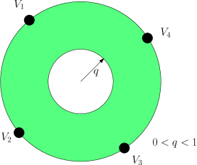
Figure 1: The one-loop planar diagram with four external states. Notice that all states are located at only one of the two boundaries of this topology, namely, the outer boundary. A non-planar diagram would have particles attached to both, outer and inner boundaries

The expressions for $P_{\pm}(q)$ above include the aforementioned factor of $(1\mp w^{1/2})^{10-D-S}$ that accounts for the projection that leaves $S$ massless scalars circulating in the loop. As an example, consider the more familiar case with D3-branes and 6 adjoint massless scalars. In this case $D=4,S=6$, gives $(1\mp w^{1/2})^{10-D-S}=1$ yielding the usual partition function. The average $\langle\cdots\rangle$ is evaluated with contractions:

$$\langle{\cal P}_{l}\rangle = \sqrt{2\alpha^{\prime}}\sum_{i}k_{i}\left[{1\over 2}\cot{\theta_{il}}+\sum_{n=1}^{\infty}{2q^{2n}\over 1-q^{2n}}\sin 2n\theta_{il}\right]$$ (19)

$$\langle{\cal P}_{i}{\cal P}_{l}\rangle-\langle{\cal P}_{i}\rangle\langle{\cal P}_{l}\rangle = {1\over 4}\csc^{2}{\theta_{il}}-\sum_{n=1}^{\infty}n{2q^{2n}\over 1-q^{2n}}\cos 2n\theta_{il}$$ (20)

$$\langle H_{i}H_{j}\rangle^{+} \equiv \chi_{+}(\theta_{ji})={1\over 2\sin\theta_{ji}}-2\sum_{r}{q^{2r}\sin 2r\theta_{ji}\over 1+q^{2r}}={1\over 2}\theta_{2}(0)\theta_{4}(0){\theta_{3}(\theta_{ji})\over\theta_{1}(\theta_{ji})}$$ (21)

$$\langle H_{i}H_{j}\rangle^{-} \equiv \chi_{-}(\theta_{ji})={\cos\theta_{ji}\over 2\sin\theta_{ji}}-2\sum_{n}{q^{2n}\sin 2n\theta_{ji}\over 1+q^{2n}}={1\over 2}\theta_{3}(0)\theta_{4}(0){\theta_{2}(\theta_{ji})\over\theta_{1}(\theta_{ji})}\;.$$ (22)

We have abbreviated $\theta_{ji}=\theta_{j}-\theta_{i}$ and space-time indices were suppressed. Finally the range of integration is

$$0=\theta_{1}<\theta_{2}<\cdots<\theta_{N}<\pi.$$ (23)

To see the GNS regulator at work, consider the one-loop 2-gluon function studied in [15] which controls the mass shifts of the gluon in perturbation theory. For the coefficient of $\epsilon_{1}\!\cdot\!\epsilon_{2}$, the bosonic part of the string amplitude is:

$$\mathcal{M}_{2}^{Bose} = \int_{0}^{1}[dq]^{\pm}\int_{0}^{\pi}d\theta\left[\sin\theta\prod_{n=1}^{\infty}\frac{1-2q^{2n}\cos 2\theta+q^{4n}}{(1-q^{2n})^{2}}\right]^{2\alpha^{\prime}k_{1}\cdot k_{2}}\times$$ (24)

$$\left[\frac{1}{4}\csc^{2}\theta-\sum_{n=1}^{\infty}n\frac{2q^{2n}}{1-q^{2n}}\cos 2n\theta\right]$$

where we use $[dq]^{\pm}$ as a short-hand for $\frac{dq}{q}\left(\frac{-\pi}{\ln q}\right)^{(10-D)/2}P_{\pm}(q)$ since this factor is not relevant for the discussion below.

Momentum conservation implies $2k_{1}\!\cdot\!k_{2}=(k_{1}+k_{2})^{2}=0$, thus

$$\mathcal{M}_{2}^{Bose} = \int_{0}^{1}[dq]\int_{0}^{\pi}d\theta\left[\frac{1}{4}\csc^{2}\theta-\sum_{n=1}^{\infty}n\frac{2q^{2n}}{1-q^{2n}}\cos 2n\theta\right]$$ (25)

from where we see that the first term is clearly divergent in the $\theta\sim 0,\pi$ regions. However, by using the GNS regulator we will show that this is a spurious divergence due to an integral representation outside its domain of convergence. In order to analytically continue the amplitude, we suspend momentum conservation in the intermediate steps by using the regulator $p=\sum_{i}k_{i}$, so that now we have $2k_{1}\!\cdot\!k_{2}=p^{2}$ instead of $2k_{1}\!\cdot\!k_{2}=0$. This makes integral perfectly convergent for ${\rm Re}(\alpha^{\prime}p^{2})>1$. We then analytically continue to $p\to 0$ at the end. Notice that there is only one angular integration in the two gluon function. This will allow us to perform the the analytic continuation to $p=0$ rather straightforwardly as we shall now see. This is in contrast with four and higher point functions where the angular integrals becomes multi-dimensional and technically more complicated. Writing (24) again, but this time with the $p$ regulator turned on, reads

$$\mathcal{M}_{2}^{Bose} = \int_{0}^{1}[dq]\int_{0}^{\pi}d\theta[\sin\theta]^{\alpha^{\prime}p^{2}}\left[\prod_{n=1}^{\infty}\frac{1-2q^{2n}\cos 2\theta+q^{4n}}{(1-q^{2}n)^{2}}\right]^{\alpha^{\prime}p^{2}}$$ (26)

$$\hskip 51.21504pt\times\left[\frac{1}{4}\csc^{2}\theta-\sum_{n=1}^{\infty}n\frac{2q^{2n}}{1-q^{2n}}\cos 2n\theta\right]$$

Expanding the infinite product up to first order in $p^{2}$ is enough for our purposes. Doing this and performing a resummation yields

$$\left[\prod_{n=1}^{\infty}\frac{1-2q^{2n}\cos 2\theta+q^{4n}}{(1-q^{2n})^{2}}\right]^{\alpha^{\prime}p^{2}}=1+\alpha^{\prime}p^{2}\sum_{m=1}^{\infty}\frac{1}{m}\frac{2q^{2m}}{1-q^{2m}}(1-\cos 2m\theta)+\mathcal{O}(p^{2})$$ (27)

therefore

$$\mathcal{M}_{2}^{Bose} = \int_{0}^{1}[dq]\left[\frac{1}{4}\int_{0}^{\pi}d\theta\,[\sin\theta]^{\alpha^{\prime}p^{2}-2}+\right.$$ (28)

$$-\sum_{n=1}^{\infty}n\frac{2q^{2n}}{1-q^{2n}}\int_{0}^{\pi}d\theta\,[\sin\theta]^{\alpha^{\prime}p^{2}}\cos 2n\theta+$$

$$+\alpha^{\prime}p^{2}\sum_{m=1}^{\infty}\frac{1}{m}\frac{2q^{2m}}{1-q^{2m}}\frac{1}{4}\int_{0}^{\pi}d\theta\,[\sin\theta]^{\alpha^{\prime}p^{2}-2}(1-\cos 2m\theta)+$$

$$\left.-\alpha^{\prime}p^{2}\sum_{m,n=1}^{\infty}\frac{1}{m}\frac{2q^{2m}}{1-q^{2m}}\frac{n2q^{2n}}{1-q^{2n}}\int_{0}^{\pi}d\theta\,[\sin\theta]^{\alpha^{\prime}p^{2}}\cos 2n\theta(1-\cos 2m\theta)\right]$$

Without the regulator, the only problematic term here is the first one, since putting $p^{2}=0$ in the integrand shows a linear divergence in the $\theta$ integration. However if we assume that ${\rm Re}(\alpha^{\prime}p^{2})>1$ we have

$$\frac{1}{4}\int_{0}^{\pi}d\theta\,[\sin\theta]^{\alpha^{\prime}p^{2}-2}=\frac{1}{4}\frac{\Gamma(1/2)\Gamma(\alpha^{\prime}p^{2}/2-1/2)}{\Gamma(\alpha^{\prime}p^{2}/2)}=-\frac{\pi\alpha^{\prime}p^{2}}{4}+\mathcal{O}(p^{4})$$ (29)

Thus, taking the right hand side to be the analytic continuation of the left-hand side as $p\to 0$, we have a convergent expression. The rest of the integrals are completely convergent even if we set $p^{2}=0$ directly in their integrands. Thus, we now have a new expression which we take it to be the analytic continuation of (24) to $p\to 0$, that reads

$$\mathcal{M}_{2}^{Bose} = \int_{0}^{1}[dq]\left[-\frac{\pi\alpha^{\prime}p^{2}}{4}+\alpha^{\prime}p^{2}\sum_{n=1}^{\infty}\frac{2q^{2n}}{1-q^{2n}}n\frac{\pi}{2n}+\alpha^{\prime}p^{2}\frac{1}{4}\sum_{m=1}^{\infty}\frac{1}{m}\frac{2q^{2m}}{1-q^{2m}}2\pi m+\right.$$ (30)

$$\left.+\alpha^{\prime}p^{2}\sum_{m=1}^{\infty}\frac{1}{m}\frac{2q^{2m}}{1-q^{2m}}\sum_{n=1}^{\infty}n\frac{2q^{2n}}{1-q^{2n}}\frac{\pi}{2}\delta_{n,m}\right]$$

$$= \pi\alpha^{\prime}p^{2}\int_{0}^{1}[dq]\left[-\frac{1}{4}+\sum_{n=1}^{\infty}\frac{q^{2n}}{1-q^{2n}}+\sum_{m=1}^{\infty}\frac{q^{2m}}{1-q^{2m}}+\sum_{n=1}^{\infty}\frac{2q^{4n}}{(1-q^{2n})^{2}}\right]$$

$$= \pi\alpha^{\prime}p^{2}\int_{0}^{1}[dq]\left[-\frac{1}{4}+\sum_{n=1}^{\infty}\frac{2q^{2n}}{(1-q^{2n})^{2}}\right]$$

which shows that, not only the limit $p\to 0$ is finite, but that it is actually zero. This is very welcome here since the vanishing of the two-gluon function guarantees that the gluon remains massless in perturbation theory, which is a consequence of gauge invariance.
The complete two-gluon amplitude is [15] given by

$$\mathcal{M}_{2}^{+} \sim \pi\alpha^{\prime}p^{2}\int[dq]^{+}\left[-\frac{1}{2}+4\sum_{n=1}^{\infty}\frac{q^{2n}}{(1-q^{2n})^{2}}+4\sum_{r=1/2}^{\infty}\frac{q^{2r}}{(1+q^{2r})^{2}}\right]$$ (31)

$$\mathcal{M}_{2}^{-} \sim \pi\alpha^{\prime}p^{2}\int[dq]^{-}\left[4\sum_{n=1}^{\infty}\frac{q^{2n}}{(1-q^{2n})^{2}}+4\sum_{n=1}^{\infty}\frac{q^{2n}}{(1+q^{2n})^{2}}\right]$$ (32)

which shows that the analytically continued result to $p\to 0$ for the full two-gluon function is indeed zero.

To motivate the general result for the $M$-gluon amplitude for the planar loop, let us consider the four gluon function. In order to be able to compare the calculations we do in this article with the results of [17] we will focus on a particular polarization structure, namely the coefficient of $\epsilon_{1}\cdot\epsilon_{4}\epsilon_{2}\cdot\epsilon_{3}$. The main reason to do this is that the coefficient of this factor is the one that dominates in the Regge limit ($s\to-\infty$ with $t$ fixed) at tree and one-loop levels. At tree level, the 4-gluon amplitude for the type 0 string (for the polarization above and omitting numerical coefficients) is

$$M_{4}^{tree}=g^{2}\frac{\Gamma(1-\alpha^{\prime}s)\Gamma(-\alpha^{\prime}t)}{\Gamma(-\alpha^{\prime}s-\alpha^{\prime}t)}$$ (33)

At one-loop the general form of the 4-gluon amplitude is given by

$$\mathcal{M}_{4}=\frac{1}{2}\left(\mathcal{M}_{4}^{+}-\mathcal{M}_{4}^{-}\right)$$ (34)

with

$$\mathcal{M}_{4}^{+} = 2^{4}\left(\frac{1}{8\pi\alpha^{\prime}}\right)^{D/2}\int_{0}^{1}\frac{dq}{q}\left(\frac{-\pi}{\ln q}\right)^{(10-D)/2}q^{-1}(1-w^{1/2})^{10-D-S}\frac{\prod_{r}^{\infty}(1+q^{2r})^{8}}{\prod_{n}^{\infty}(1-q^{2n})^{8}}$$ (35)

$$\int\prod_{k=2}^{4}d\theta_{k}\prod_{i<j}[\psi(\theta_{ji})]^{2\alpha^{\prime}k_{i}\cdot k_{j}}\langle\hat{\mathcal{P}}_{1}\hat{\mathcal{P}}_{2}\hat{\mathcal{P}}_{3}\hat{\mathcal{P}}_{4}\rangle^{+}$$

$$\mathcal{M}_{4}^{-} = 2^{4}\left(\frac{1}{8\pi\alpha^{\prime}}\right)^{D/2}\int_{0}^{1}\frac{dq}{q}\left(\frac{-\pi}{\ln q}\right)^{(10-D)/2}2^{4}(1+w^{1/2})^{10-D-S}\frac{\prod_{r}^{\infty}(1+q^{2n})^{8}}{\prod_{n}^{\infty}(1-q^{2n})^{8}}$$ (36)

$$\int\prod_{k=2}^{4}d\theta_{k}\prod_{i<j}[\psi(\theta_{ji})]^{2\alpha^{\prime}k_{i}\cdot k_{j}}\langle\hat{\mathcal{P}}_{1}\hat{\mathcal{P}}_{2}\hat{\mathcal{P}}_{3}\hat{\mathcal{P}}_{4}\rangle^{-}$$

Picking out the combination that multiplies $\epsilon_{1}\cdot\epsilon_{4}\epsilon_{2}\cdot\epsilon_{3}$ from the corrrelator gives

$$\langle{\hat{\cal P}}_{1}{\hat{\cal P}}_{2}{\hat{\cal P}}_{3}{\hat{\cal P}}_{4}\rangle \to \epsilon_{2}\cdot\epsilon_{3}\epsilon_{1}\cdot\epsilon_{4}\bigg{(}\langle{{\cal P}}_{2}{{\cal P}}_{3}\rangle\langle{{\cal P}}_{1}{{\cal P}}_{4}\rangle-\langle{{\cal P}}_{2}{{\cal P}}_{3}\rangle\langle H_{1}H_{4}\rangle^{2}2\alpha^{\prime}k_{1}\cdot k_{4}$$ (37)

$$\hskip-72.26999pt-\langle{{\cal P}}_{1}{{\cal P}}_{4}\rangle\langle H_{2}H_{3}\rangle^{2}2\alpha^{\prime}k_{2}\cdot k_{3}+4\alpha^{\prime 2}\langle H_{2}H_{3}\rangle\langle H_{1}H_{4}\rangle\langle k_{1}\cdot H_{1}k_{2}\cdot H_{2}k_{3}\cdot H_{3}k_{4}\cdot H_{4}\rangle\bigg{)}$$

$$\to \epsilon_{2}\cdot\epsilon_{3}\epsilon_{1}\cdot\epsilon_{4}\bigg{(}\langle{{\cal P}}_{2}{{\cal P}}_{3}\rangle\langle{{\cal P}}_{1}{{\cal P}}_{4}\rangle-\langle{{\cal P}}_{2}{{\cal P}}_{3}\rangle\langle H_{1}H_{4}\rangle^{2}2\alpha^{\prime}k_{1}\cdot k_{4}$$

$$\hskip-72.26999pt-\langle{{\cal P}}_{1}{{\cal P}}_{4}\rangle\langle H_{2}H_{3}\rangle^{2}2\alpha^{\prime}k_{2}\cdot k_{3}+4\alpha^{\prime 2}\langle H_{2}H_{3}\rangle\langle H_{1}H_{4}\rangle(k_{1}\cdot k_{2}k_{3}\cdot k_{4}\langle H_{1}H_{2}\rangle\langle H_{3}H_{4}\rangle$$

$$-k_{1}\cdot k_{3}k_{2}\cdot k_{4}\langle H_{1}H_{3}\rangle\langle H_{2}H_{4}\rangle+k_{1}\cdot k_{4}k_{2}\cdot k_{3}\langle H_{2}H_{3}\rangle\langle H_{1}H_{4}\rangle\bigg{)}$$

$$\to \epsilon_{2}\cdot\epsilon_{3}\epsilon_{1}\cdot\epsilon_{4}\bigg{(}(\langle{{\cal P}}_{2}{{\cal P}}_{3}\rangle+\alpha^{\prime}t\langle H_{2}H_{3}\rangle^{2})(\langle{{\cal P}}_{1}{{\cal P}}_{4}\rangle+\alpha^{\prime}t\langle H_{1}H_{4}\rangle^{2})$$

$$\hskip-72.26999pt+\langle H_{2}H_{3}\rangle\langle H_{1}H_{4}\rangle(\alpha^{\prime 2}s^{2}\langle H_{1}H_{2}\rangle\langle H_{3}H_{4}\rangle-\alpha^{\prime 2}(s+t)^{2}\langle H_{1}H_{3}\rangle\langle H_{2}H_{4}\rangle)\bigg{)}$$

We will call this combination of contractions $\langle T\rangle$, hence

$$\langle T\rangle \equiv \left(\langle{{\cal P}}_{2}{{\cal P}}_{3}\rangle+\alpha^{\prime}t\langle H_{2}H_{3}\rangle^{2}\right)\left(\langle{{\cal P}}_{1}{{\cal P}}_{4}\rangle+\alpha^{\prime}t\langle H_{1}H_{4}\rangle^{2}\right)$$ (38)

$$+\langle H_{2}H_{3}\rangle\langle H_{1}H_{4}\rangle\left(\alpha^{\prime 2}s^{2}\langle H_{1}H_{2}\rangle\langle H_{3}H_{4}\rangle-\alpha^{\prime 2}(s+t)^{2}\langle H_{1}H_{3}\rangle\langle H_{2}H_{4}\rangle\right)$$

thus, the correlator becomes

$$\langle{\hat{\cal P}}_{1}{\hat{\cal P}}_{2}{\hat{\cal P}}_{3}{\hat{\cal P}}_{4}\rangle\to\epsilon_{1}\!\cdot\!\epsilon_{4}\,\epsilon_{2}\!\cdot\!\epsilon_{3}\,\langle T\rangle$$ (39)

As pointed out before, the expressions (35) and (36) diverge in various corners of integration region over the $\theta_{k}$ variables. We already encountered a divergence of the linear type in the 2-gluon amplitude due to the behavior of $(\csc\theta)^{2}$ near the end points $\theta\sim 0,\pi$. We showed that this divergence was spurious and it was healed by suspending momentum conservation in $\sum_{i=1}^{M}p_{i}=p\neq 0$ temporarily. After that, we were able to identify the integral in (29) as the Euler Beta function which allowed us to analytically continue the left hand side to the complete complex $p$-plane. Undoubtedly, for the three and higher point amplitudes a closed form is practically impossible to obtain. However, our approach to the problem will not be to attempt this, but to extract the divergent contributions from the singular regions and track the consequences of these seemingly divergent terms. What we will find is that the analytic continuation to $p=0$ of the linearly divergent terms precisely combine and give the tree amplitude following the steps of [34]. Although the coefficient of this term is an infinite number (which can also be viewed due to the presence of the closed string tachyon which introduces a singularity in the $q\sim 0$ region), the fact that it is proportional to the tree amplitude allows us re-interpret it as a renormalization of the string coupling constant. We will then find that the logarithmically divergent corners, when continued to $p=0$ also produce terms proportional to the tree amplitude, although in this case the coefficient in front of it is a finite number and these corners will simply correct the coupling by a finite amount. We will now make these statements more explicit with the following calculations.

2.2 Linear Divergences

We will now extract the leading divergences in the $\theta_{k}$ integrations at fixed $q$ and show that they are linear divergences in the relevant angular variables. We construct the necessary counterterms to cancel these infinities and show that after analytic continuation, the limit $p\to 0$ of the angular integrals is finite. We will follow closely the analysis done by Neveu and Scherk [34] adapted for our case, open string massless vector external states (’gluons’) in the type 0 model, and show that not only the limit is finite, but also that its continuation to $p\to 0$ gives precisely the tree amplitude. This allows us to absorb the corresponding counterterms into the open string coupling.

For the $M$-point planar one-loop amplitude, the integration region in $\int\prod_{k}d\theta_{k}$ is given by $0<\theta_{2}<\theta_{3}<\cdots<\theta_{M}<\pi$, which is an $(M-1)$-simplex that has $M$ vertices and $M!/2!(M-2)!$ edges. For example, the integration region over the $\theta_{k}$ variables for the 4-point amplitude is shown in figure 2.

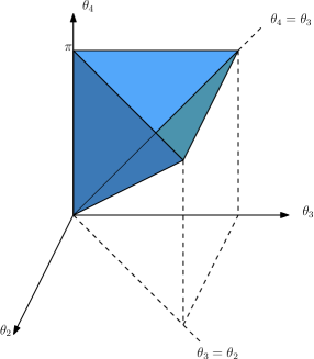
Figure 2: The 3-simplex above shows the region of integration at fixed $q$ for the 4-point amplitude. Edges and vertices correspond to the places where spurious and real divergences can occur.

The leading divergences are linear and arise from each of the $M$ vertices in the $M$-gluon amplitude as we will show next.

We can study the vertices of the ($M-1$)-simplex by remembering that they correspond to the configuration in parameter space where all the vertex operators coincide (see figure 3 which shows the 4-point case).

Figure 3: Configuration corresponding to the moduli region where all vertex operators come arbitrarily close to each other.

For instance, we can examine the one where $\theta_{M}\sim\theta_{M-1}\sim\cdots\sim\theta_{2}\sim 0$ by studying the $\theta_{M}\sim 0$ limit and performing the changes

$$\theta_{j-1} \equiv \theta_{j}\hat{\theta}_{j-1}\quad j=3,\cdots M$$ (40)

For the 4-gluon amplitude, and keeping only the most divergent terms in the $\theta_{k}$ integrations, we have

$$\prod_{i<j}\psi(\theta_{ji})^{2\alpha^{\prime}k_{i}\cdot k_{j}} \simeq \theta_{4}^{\alpha^{\prime}p^{2}}\hat{\theta}_{3}^{2\alpha^{\prime}k_{4}\cdot p}(1-\hat{\theta}_{3})^{2\alpha^{\prime}k_{4}\cdot k_{3}}(1-\hat{\theta}_{3}\hat{\theta}_{2})^{2\alpha^{\prime}k_{4}\cdot k_{2}}\hat{\theta}_{2}^{2\alpha^{\prime}k_{2}\cdot k_{1}}(1-\hat{\theta}_{2})^{2\alpha^{\prime}k_{3}\cdot k_{2}}$$

where we have also only kept the leading terms in $p$ in the exponents. Also

$$\langle T\rangle^{+} \simeq \frac{1}{4\theta_{4}^{2}}(1+\alpha^{\prime}t)\frac{1}{4\theta_{32}}(1+\alpha^{\prime}t)+\frac{1}{2\theta_{4}}\frac{1}{2\theta_{32}}\left[(\alpha^{\prime}s)^{2}\frac{1}{2\theta_{2}}\frac{1}{2\theta_{43}}-\alpha^{\prime 2}(s+t)^{2}\frac{1}{2\theta_{3}}\frac{1}{2\theta_{42}}\right]$$ (42)

$$\simeq \frac{1}{16\,\theta_{4}^{4}\hat{\theta}_{3}^{2}(1-\hat{\theta}_{2})}\left[\frac{(1+\alpha^{\prime}t)^{2}}{1-\hat{\theta}_{2}}+\frac{(\alpha^{\prime}s)^{2}}{\hat{\theta}_{2}(1-\hat{\theta}_{3})}-\frac{\alpha^{\prime 2}(s+t)^{2}}{1-\hat{\theta}_{3}\hat{\theta}_{2}}\right]$$

thus

$$\int_{0}^{\epsilon}d\theta_{4}\int_{0}^{\theta_{4}}d\theta_{3}\int_{0}^{\theta_{3}}d\theta_{2}\prod_{i<j}\psi(\theta_{ji})^{2\alpha^{\prime}k_{i}\cdot k_{j}}\langle T\rangle^{+}\simeq$$ (43)

$$\simeq \frac{1}{16}\int_{0}^{\epsilon}d\theta_{4}\theta_{4}^{\alpha^{\prime}p^{2}-2}\int_{0}^{1}d\hat{\theta}_{3}\hat{\theta}_{3}^{2\alpha^{\prime}k_{4}\cdot p-1}(1-\hat{\theta}_{3})^{2\alpha^{\prime}k_{4}\cdot k_{3}}\int_{0}^{1}d\hat{\theta}_{2}\hat{\theta}_{2}^{2\alpha^{\prime}k_{2}\cdot k_{1}}(1-\hat{\theta}_{2})^{2\alpha^{\prime}k_{3}\cdot k_{2}-1}$$

$$\times(1-\hat{\theta}_{3}\hat{\theta}_{2})^{2\alpha^{\prime}k_{4}\cdot k_{2}}\left[\frac{(1+\alpha^{\prime}t)^{2}}{1-\hat{\theta}_{2}}+\frac{(\alpha^{\prime}s)^{2}}{\hat{\theta}_{2}(1-\hat{\theta}_{3})}-\frac{\alpha^{\prime 2}(s+t)^{2}}{1-\hat{\theta}_{3}\hat{\theta}_{2}}\right]$$

from which we see that, if we put $p=0$ directly in the integrand, the leading divergence near $\theta_{4}=0$ is linear. It is worth noticing that in this corner of the integration region the integral factorizes and shows a pole at $\alpha^{\prime}p^{2}=1$ which corresponds to the propagation of a closed string tachyon disappearing into the vacuum. In contrast to superstring theories where this kind of divergences are absent due to supersymmetry, the planar one-loop diagram in the type 0 model is not divergence free, but it is renormalizable [37]. The cancellation of these divergences is achieved with the introduction of counter-terms just as in the early days of the dual resonance models. We now proceed to cancel this and all of the other linear divergences which come from all the vertices of the simplex with one single counter-term. We subtract and add back the following counter-term:

$$C_{4}^{+}\equiv 2^{4}\left(\frac{1}{8\pi^{2}\alpha^{\prime}}\right)^{D/2}\int_{0}^{1}[dq]^{+}\int\prod_{k=2}^{4}d\theta_{k}\prod_{i<j}[\sin\theta_{ji}]^{2\alpha^{\prime}k_{i}\cdot k_{j}}\langle T\rangle^{+}_{C}$$ (44)

where $\langle T\rangle^{+}_{C}$ is simply $\langle T\rangle^{+}$ evaluated at $q=0$. Following Neveu and Scherk [34], we will now prove that the analytic continuation to $p=0$ of $C_{4}^{+}$ goes to the tree amplitude (33). Making the change of integration variables

$$r(\theta_{3})=\frac{\sin\theta_{43}}{\sin\theta_{3}}\,\qquad x(\theta_{2})=\frac{\sin\theta_{2}\sin\theta_{43}}{\sin\theta_{3}\sin\theta_{42}}$$ (45)

and solving for the various sine functions we need in the integrand, yields

$$\sin\theta_{43} =\frac{r\sin\theta_{4}}{\sqrt{r^{2}+2r\cos\theta_{4}+1}}\quad \sin\theta_{42} =\frac{r/x\sin\theta_{4}}{\sqrt{(r/x)^{2}+2r/x\cos\theta_{4}+1}}$$

$$\sin\theta_{32} =\frac{r/x(1-x)\sin\theta_{4}}{\sqrt{(r/x)^{2}+2r/x\cos\theta_{4}+1}\sqrt{r^{2}+2r\cos\theta_{4}+1}}\quad \sin\theta_{3} =\frac{\sin\theta_{4}}{\sqrt{r^{2}+2r\cos\theta_{4}+1}}$$

$$\sin\theta_{2} =\frac{\sin\theta_{4}}{\sqrt{(r/x)^{2}+2r/x\cos\theta_{4}+1}}$$ (46)

Thus,

$$\prod_{i<j}[\sin\theta_{ji}]^{2\alpha^{\prime}k_{i}\cdot k_{j}} = r^{2\alpha^{\prime}k_{1}\cdot p+\alpha^{\prime}p^{2}}[\sin\theta_{4}]^{\alpha^{\prime}p^{2}}\left(r^{2}+2r\cos\theta_{4}+1\right)^{\alpha^{\prime}k_{3}\cdot p}\left(\frac{r^{2}}{x^{2}}+\frac{2r}{x}\cos\theta_{4}+1\right)^{\alpha^{\prime}k_{2}\cdot p}$$ (47)

$$\times\,x^{-\alpha^{\prime}s+2\alpha^{\prime}k_{2}\cdot p}(1-x)^{-\alpha^{\prime}t}$$

$$d\theta_{3}d\theta_{2} = r\,[\sin\theta_{4}]^{2}(r^{2}+2r\cos\theta_{4}+1)^{-1}\left(\frac{r^{2}}{x^{2}}+\frac{2r}{x}\cos\theta_{4}+1\right)^{-1}x^{-2}dr\,dx$$ (48)

$$\langle T\rangle_{C}^{+} = \frac{1}{16}\csc^{2}\theta_{4}\csc^{2}\theta_{32}(1+\alpha^{\prime}t)^{2}+$$ (49)

$$+\frac{1}{4}\csc\theta_{4}\csc\theta_{32}\left[\frac{(\alpha^{\prime}s)^{2}}{4}\csc\theta_{2}\csc\theta_{43}-\frac{\alpha^{\prime 2}(s+t)^{2}}{4}\csc\theta_{3}\csc\theta_{42}\right]$$

$$= \frac{1}{16}r^{-2}[\sin\theta_{4}]^{-4}(r^{2}+2r\cos\theta_{4}+1)\left(\frac{r^{2}}{x^{2}}+\frac{2r}{x}\cos\theta_{4}+1\right)$$

$$\times\left[(1+\alpha^{\prime}t)^{2}\frac{x^{2}}{(1-x)^{2}}+(\alpha^{\prime}s)^{2}\frac{x}{1-x}-\alpha^{\prime 2}(s+t)^{2}\frac{x^{2}}{1-x}\right]$$

Therefore,

$$\int\prod_{k=2}^{4}d\theta_{k}\prod_{i<j}[\sin\theta_{ji}]^{2\alpha^{\prime}k_{i}\cdot k_{j}}\langle T\rangle^{+}_{C}=$$ (50)

$$= \frac{1}{16}\int_{0}^{1}\!\!dx\int_{0}^{\infty}\!\!dr\int_{0}^{\pi}\!\!d\theta_{4}\,r^{2\alpha^{\prime}k_{1}\cdot p+\alpha^{\prime}p^{2}-1}[\sin\theta_{4}]^{\alpha^{\prime}p^{2}-2}x^{-\alpha^{\prime}s}(1-x)^{-\alpha^{\prime}t}(r^{2}+2r\cos\theta_{4}+1)^{\alpha^{\prime}k_{3}\cdot p}$$

$$\times\left(\frac{r^{2}}{x^{2}}+\frac{2r}{x}\cos\theta_{4}+1\right)^{\alpha^{\prime}k_{2}\cdot p}\left[(1+\alpha^{\prime}t)^{2}\frac{x^{2}}{(1-x)^{2}}+(\alpha^{\prime}s)^{2}\frac{x}{1-x}-\alpha^{\prime 2}(s+t)^{2}\frac{x^{2}}{1-x}\right]$$

The strategy is to do the integrals in the following order: first we do the integration over $\theta_{4}$, then the one over $r$ and at the end, after the analytic continuation to $p\to 0$ has been achieved, we perform the integral over $x$. It is because of this that we have used $-\alpha^{\prime}s+2\alpha^{\prime}k_{2}\cdot p\to-\alpha^{\prime}s$ since we can always choose $-\alpha^{\prime}s$ to be positive enough such that the integral over $x$ in convergent. Let us now focus on the integrals over $r$ and $\theta_{4}$. For this purpose, define

$$I \equiv \int_{0}^{\infty}dr\,r^{2\alpha^{\prime}k_{1}\cdot p+\alpha^{\prime}p^{2}-1}\int_{0}^{\pi}d\theta_{4}[\sin\theta_{4}]^{\alpha^{\prime}p^{2}-2}(r^{2}+2r\cos\theta_{4}+1)^{\alpha^{\prime}k_{3}\cdot p}$$ (51)

$$\times\left(\frac{r^{2}}{x^{2}}+\frac{2r}{x}\cos\theta_{4}+1\right)^{\alpha^{\prime}k_{2}\cdot p}$$

As $p\to 0$, the only non-zero contributions to the integral come from only two corners [34]: $\theta_{4}\sim\pi$ and $r$ is near either $r=1$ or $r=x$. Each corner gives the same answer which is $\pi$, therefore:

$$I\to 2\pi\quad\mbox{as $p\to 0$}$$ (52)

Therefore,

$$\int\prod_{k=2}^{4}d\theta_{k}\prod_{i<j}[\sin\theta_{ji}]^{2\alpha^{\prime}k_{i}\cdot k_{j}}\langle T\rangle^{+}_{C}=$$ (53)

$$= \frac{2\pi}{16}\int_{0}^{1}dx\,x^{-\alpha^{\prime}s}(1-x)^{-\alpha^{\prime}t}\left[(1+\alpha^{\prime}t)^{2}\frac{x^{2}}{(1-x)^{2}}+(\alpha^{\prime}s)^{2}\frac{x}{1-x}-\alpha^{\prime 2}(s+t)^{2}\frac{x^{2}}{1-x}\right]$$

$$= -\frac{\pi}{8}\frac{\Gamma(1-\alpha^{\prime}s)\Gamma(-\alpha^{\prime}t)}{\Gamma(-\alpha^{\prime}s-\alpha^{\prime}t)}$$

from where we see that this is precisely proportional to the tree amplitude (33). Therefore, after analytic continuation to $p=0$, the counter-term $C_{4}^{+}$ becomes:

$$C_{4}^{+} = \!\!\!-\frac{\pi}{4}\underbrace{\frac{\Gamma(1-\alpha^{\prime}s)\Gamma(-\alpha^{\prime}t)}{\Gamma(-\alpha^{\prime}s-\alpha^{\prime}t)}}_{\text{Tree}}\left(\frac{1}{8\pi\alpha^{\prime}}\right)^{D/2}\int_{0}^{1}\frac{dq}{q}\left(\frac{-\pi}{\ln q}\right)^{(10-D)/2}\!\!\!\!\!\!\!q^{-1}(1-w^{1/2})^{10-D-S}\frac{\prod_{r}^{\infty}(1+q^{2r})^{8}}{\prod_{n}^{\infty}(1-q^{2n})^{8}}$$

As mentioned before, the counter-term is the product of the tree amplitude and a divergent factor. This infinity comes from the divergent region $q=0$ in the expression above which signals the presence of the tachyon in the closed string sector. This counter-term was originally introduced in [34] and [38] to precisely cancel this type of divergence, and the fact that it is proportional to the tree amplitude here allows us to absorb this divergence into a coupling constant renormalization. The remarkable feature of this counter-term is that it allows to cancel both, the $q=0$ singularity, and the spurious linear divergences of the $\theta_{k}$ integrations at the same time. This is a consequence of the functional form of the correlator $\langle\hat{\mathcal{P}}_{1}\cdots\hat{\mathcal{P}}_{M}\rangle$ since the $\theta^{-2}$ divergent terms that arise from the $\csc^{2}\theta$ functions only come from the $q=0$ part of Wick expansion of $\langle\hat{\mathcal{P}}_{1}\cdots\hat{\mathcal{P}}_{M}\rangle$. We thus now have a new expression free of both, the spurious linear divergences in the $\theta_{k}$ variables, and the UV one coming from $q=0$. Therefore, our expressions for the + part of the amplitude need the replacement

$$\mathcal{M}_{4}^{+}\to\mathcal{M}_{4}^{+}-C_{4}^{+}$$ (54)

Now we need to address the $\mathcal{M}_{4}^{-}$ part of the amplitude. Notice in (14) that the presence of D-branes, which brings the extra logarithmic factor $\left(\frac{-\pi}{\ln q}\right)^{(10-D)/2}$, makes the $q$-integration completely finite near $q=0$ as long as $D<8$ and hence there is no need for a counterterm for the $\mathcal{M}_{4}^{-}$ part of the amplitude. However, we still need to deal with the same linear and logarithmic divergences in the $\theta_{k}$ integration as in the $\mathcal{M}_{4}^{+}$ case. For the leading divergences, the natural choice would be the same one we used for the $\mathcal{M}_{4}^{+}$ case, but now with $\langle\hat{\mathcal{P}}_{1}\cdots\hat{\mathcal{P}}_{M}\rangle^{+}$ replaced by $\langle\hat{\mathcal{P}}_{1}\cdots\hat{\mathcal{P}}_{M}\rangle^{-}$. However, we have not been able to obtain the analytic continuation to $p=0$ for such an expression. The main difficulty comes from the fact that the $\langle\hat{\mathcal{P}}_{1}\cdots\hat{\mathcal{P}}_{M}\rangle^{-}$ correlators involve $\cot\theta_{ji}$ functions which change sign in the integration region $0<\theta_{2}<\cdots<\theta_{M}<\pi$. This did not happen for the + correlators since they contain $\sin\theta_{ji}$ functions instead.

However, since we only need to cancel the linear divergences, we simply choose the same correlator as before, i.e., $\langle\hat{\mathcal{P}}_{1}\cdots\hat{\mathcal{P}}_{M}\rangle^{+}$. Thus, we only need to adapt the counter-term for the $\mathcal{M}^{-}$ part of the amplitude by integrating with the $[dq]^{-}$ measure. This means that we choose:

$$C_{4}^{-}\equiv 2^{4}\left(\frac{1}{8\pi^{2}\alpha^{\prime}}\right)^{D/2}\int_{0}^{1}[dq]^{-}\int\prod_{k=2}^{4}d\theta_{k}\prod_{i<j}[\sin\theta_{ji}]^{2\alpha^{\prime}k_{i}\cdot k_{j}}\langle T\rangle^{+}_{C}$$ (55)

Summarizing, we now write $\mathcal{M}_{4}^{\pm}$ as:

$$\mathcal{M}_{4}^{\pm}=\mathcal{M}_{4}^{\pm}-\mathcal{C}_{4}^{\pm}+\mathcal{C}_{4}^{\pm}$$ (56)

The last term will be discarded later on since we are going to absorb it into a coupling constant renormalization. The full expression for the first two terms is then:

$$\mathcal{M}_{4}^{\pm}-\mathcal{C}_{4}^{\pm} = 2^{4}\left(\frac{1}{8\pi^{2}\alpha^{\prime}}\right)^{D/2}\!\!\!\int_{0}^{1}[dq]^{\pm}\int\prod_{k=2}^{4}d\theta_{k}\prod_{i<j}\left[\psi(\theta_{ji})^{2\alpha^{\prime}k_{i}\cdot k_{j}}\langle T\rangle^{\pm}-[\sin\theta_{ji}]^{2\alpha^{\prime}k_{i}\cdot k_{j}}\langle T\rangle^{\pm}_{C}\right]$$ (57)

The expression above is completely free of both, the spurious linear divergences in the $\theta_{k}$ integrations and the UV divergence from the $q\sim 0$ region. However, it still has logarithmic divergences in the $\theta_{k}$ integration which we take care of in the next section. We will show that they are also spurious divergences and can be also cancelled with the introduction of suitable counterterms. Moreover, after analytic continuation to $p=0$, we will show that the corresponding counterterms are again proportional to the tree level amplitude which amounts to a finite renormalization of the coupling.

2.3 Logarithmic Divergences

The expression (57) is the starting point to continue our treatment of the divergences of the original ‘bare’ amplitude. Our task now is to study the last type of divergences in the $\theta_{k}$ integrals left in (57), which are logarithmic.

Logarithmic divergences in the angular integrations come from the regions where all vertex operators but one come together in parameter space. It is a well-known fact that these divergences correspond to loop corrections to the mass of the external states. Since we are dealing with massless string states, we expect these divergences to be completely absent after continuation to $p=0$ because the massless vector string states must remain massless in perturbation theory due to gauge invariance. We will indeed find this result for the $4$-gluon amplitude. The mechanics of the procedure is very well illustrated by the 4-gluon amplitude and will allow us to see how to extend it for an arbitrary number of gluons.

Recall that for the $M$-gluon amplitude the integration region over $\theta_{k}$ is an $(M-1)$-simplex, which has $M!/(2!(M-2)!)$ edges (see figure 2 for the 4-gluon amplitude in which case there are 6 edges). Each of these edges correspond to processes where an open string loop is inserted between two string states. If one of these states correspond to one of the $M$ external states, then we have the situation where an internal propagator gets evaluated on-shell, producing an infinity. Before proceeding with the analysis of these infinities, let us do some counting first. We see that there are

$$\frac{M!}{2!(M-2)!}-M=\frac{M}{2}(M-3)$$ (58)

edges left which do not correspond to radiative corrections to the external legs. Therefore, the number of edges that correspond to a loop insertion in the internal channels of the $M$-gluon amplitude has to be given by equation (58). On the other hand, we know that the number of planar channels in an $M$-point string amplitude is $M/2(M-3)$ which precisely matches the number above.

Let us now focus on the 4-gluon amplitude. This has four (out of six) edges that should correspond to an open string loop inserted for each external leg. We now study one of them, namely the edge $\theta_{3}\sim\theta_{2}\sim 0$ which is highlighted in figure 4.

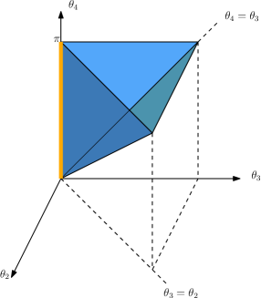
Figure 4: The edge corresponding to $\theta_{3}\sim\theta_{2}\sim 0$ is shown as the highlighted line in the figure. This region corresponds to a loop insertion in one of the external states which forces the propagator for state number 4 to be evaluated on-shell producing a divergence

This corresponds to the region where the vertex operators associated with external states 1, 2 and 3 get close together in parameter space and it reflects a radiative correction to the mass of the external leg 4. To analyze this region, it is convenient to make the change $\theta_{2}\equiv\theta_{3}\hat{\theta}_{2}$ and study the small $\theta_{3}$ behavior, namely

$$\prod_{i<j}\psi(\theta_{ji})^{2\alpha^{\prime}k_{i}\cdot k_{j}} \simeq \psi(\theta_{4})^{-2\alpha^{\prime}k_{4}\cdot p}\theta_{3}^{2\alpha^{\prime}k_{4}\cdot p+\alpha^{\prime}p^{2}}\hat{\theta}_{2}^{-\alpha^{\prime}s}(1-\hat{\theta}_{2})^{-\alpha^{\prime}t}$$ (59)

and also

$$\langle T\rangle \simeq \left(\mathcal{P}_{14}+\alpha^{\prime}t\langle H_{1}H_{4}\rangle^{2}\right)(1+\alpha^{\prime}t)\frac{1}{4\theta_{32}^{2}}+\langle H_{1}H_{4}\rangle^{2}\frac{1}{2\theta_{32}}\left[\frac{(\alpha^{\prime}s)^{2}}{2\theta_{2}}-\frac{\alpha^{\prime 2}(s+t)^{2}}{2\theta_{3}}\right]$$

$$= \frac{1}{4\theta_{3}^{2}}\left[\mathcal{P}_{14}\frac{(1+\alpha^{\prime}t)}{(1-\hat{\theta}_{2})^{2}}+\langle H_{1}H_{4}\rangle^{2}\left(\frac{\alpha^{\prime}t(1+\alpha^{\prime}t)}{(1-\hat{\theta}_{2})^{2}}+\frac{(\alpha^{\prime}s)^{2}}{\hat{\theta}_{2}(1-\hat{\theta}_{2})}-\frac{\alpha^{\prime 2}(s+t)^{2}}{(1-\hat{\theta}_{2})}\right)\right]$$

From $\prod_{k=2}^{4}d\theta_{k}=d\theta_{3}\theta_{3}d\hat{\theta}_{2}$ and equations (59) and (LABEL:corredge1), we see that the leading behavior of the integral over the three angles separates into three independent integrals. The integration over the $\theta_{k}$ variables in (57) becomes

$$\int\prod_{k=2}^{4}d\theta_{k}\left[\prod_{i<j}\psi(\theta_{ji})^{2\alpha^{\prime}k_{i}\cdot k_{j}}\langle T\rangle^{\pm}-\prod_{i<j}[\sin\theta_{ji}]^{2\alpha^{\prime}k_{i}\cdot k_{j}}\langle T\rangle^{\pm}_{C}\right]=$$

$$\simeq \frac{1}{4}\int_{0}^{\pi}d\theta_{4}\int_{0}^{\epsilon}d\theta_{3}\int_{0}^{1}d\hat{\theta}_{2}\,\psi(\theta_{4})^{-2\alpha^{\prime}k_{4}\cdot p}\,\theta_{3}^{2\alpha^{\prime}k_{4}\cdot p+\alpha^{\prime}p^{2}-1}\,\hat{\theta}_{2}^{-\alpha^{\prime}s}(1-\hat{\theta}_{2})^{-\alpha^{\prime}t}$$

$$\times\left[(\mathcal{P}_{14}-\mathcal{P}_{14C})\frac{(1+\alpha^{\prime}t)}{(1-\hat{\theta}_{2})^{2}}\right.$$

$$\hskip 50.0pt\left.+(\langle H_{1}H_{4}\rangle^{2}-\langle H_{1}H_{4}\rangle_{C}^{2})\left(\frac{\alpha^{\prime}t(1+\alpha^{\prime}t)}{(1-\hat{\theta}_{2})^{2}}+\frac{(\alpha^{\prime}s)^{2}}{\hat{\theta}_{2}(1-\hat{\theta}_{2})}-\frac{\alpha^{\prime 2}(s+t)^{2}}{(1-\hat{\theta}_{2})}\right)\right]$$

If we take $p=0$ in the integrand, i.e., if we go back to the original calculation before the introduction of the GNS regulator, we see the logarithmic divergence

$$\int_{0}^{\epsilon}d\theta_{3}\,\theta_{3}^{-1}$$ (62)

Notice that

$$\mathcal{P}_{14}-\mathcal{P}_{14C}=\mathcal{O}(1)\quad\text{and}\quad\langle H_{1}H_{4}\rangle^{2}-\langle H_{1}H_{4}\rangle_{C}^{2}=\mathcal{O}(1)$$ (63)

as $\theta_{4}\to 0,\pi$, thus there are no linear divergences near this edge either, which is simply a consequence of the subtraction made in the previous subsection that was introduced precisely to get rid of this type of divergences. Therefore, we need to subtract (LABEL:intedge1), evaluated at $p=0$, from (57) and we will have a new expression which is free from all linear and the one logarithmic divergence that arises from the $\theta_{3}\sim\theta_{2}\sim 0$ edge. Let us write this new expression in terms of the original $\theta$ variables as

$$\int_{0}^{\pi}d\theta_{4}\int_{0}^{\theta_{4}}d\theta_{3}\int_{0}^{\theta_{3}}d\theta_{2}\left[\prod_{i<j}\psi(\theta_{ji})^{2\alpha^{\prime}k_{i}\cdot k_{j}}\langle T\rangle^{\pm}-\prod_{i<j}[\sin\theta_{ji}]^{2\alpha^{\prime}k_{i}\cdot k_{j}}\langle T\rangle^{\pm}_{C}-B_{4}\right]$$

where $B_{4}$ denotes the integrand corresponding to the loop insertion on leg 4 which, in the new variables, is

$$B_{4}\!\!\!\! = \!\!\!\!\frac{1}{4}\,\theta_{3}^{2\alpha^{\prime}k_{4}\cdot p+\alpha^{\prime}p^{2}-1}\,\hat{\theta}_{2}^{-\alpha^{\prime}s}(1-\hat{\theta}_{2})^{-\alpha^{\prime}t}\left[\left(\mathcal{P}(\theta_{4})-\mathcal{P}(\theta_{4})_{C}\right)\frac{(1+\alpha^{\prime}t)}{(1-\hat{\theta}_{2})^{2}}+\right.$$

$$\left.+\left(\chi_{+}^{2}(\theta_{4})-\chi_{+}^{2}(\theta_{4})_{C}\right)\left(\frac{\alpha^{\prime}t(1+\alpha^{\prime}t)}{(1-\hat{\theta}_{2})^{2}}+\frac{(\alpha^{\prime}s)^{2}}{\hat{\theta}_{2}(1-\hat{\theta}_{2})}-\frac{\alpha^{\prime 2}(s+t)^{2}}{(1-\hat{\theta}_{2})}\right)\right]$$

Now that we have taken care of the divergence by subtracting the counterterm $B_{4}$, let us see what is the result of the analytic continuation to $p=0$ when we add this term back. With the GNS regulator put back on, we now need to compute

$$\int_{0}^{\pi}d\theta_{4}\int_{0}^{\theta_{4}}d\theta_{3}\int_{0}^{1}d\hat{\theta}_{2}\,\psi(\theta_{4})^{-2\alpha^{\prime}k_{4}\cdot p}\,B_{4}(\theta_{4}.\theta_{3},\hat{\theta}_{2})$$ (66)

and then we need to perform on this expression the analytic continuation to $p=0$. The integral over $\theta_{3}$ is

$$\int_{0}^{\theta_{4}}d\theta_{3}\,\theta_{3}^{2\alpha^{\prime}k_{4}\cdot p+\alpha^{\prime}p^{2}-1}=\frac{\theta_{4}^{2\alpha^{\prime}k_{4}\cdot p+\alpha^{\prime}p^{2}}}{2\alpha^{\prime}k_{4}\cdot p+\alpha^{\prime}p^{2}}\to\frac{\theta_{4}^{2\alpha^{\prime}k_{4}\cdot p}}{2\alpha^{\prime}k_{4}\cdot p}$$ (67)

as $p\to 0$. We will now solve for the rest of the integrals. We will find that the integral over $\theta_{4}$ precisely vanishes as $\mathcal{O}(\alpha^{\prime}k_{4}\cdot p)$, cancelling the $\frac{1}{2\alpha^{\prime}k_{4}\cdot p}$ pole in (67), thus giving a finite result which is exactly what we desire. Proceeding this way, we have

$$\frac{1}{8\alpha^{\prime}k_{4}\cdot p}\int_{0}^{\pi}d\theta_{4}\int_{0}^{1}d\hat{\theta}_{2}\,\psi(\theta_{4})^{-2\alpha^{\prime}k_{4}\cdot p}\,\theta_{4}^{2\alpha^{\prime}k_{4}\cdot p}\hat{\theta}_{2}^{-\alpha^{\prime}s}(1-\hat{\theta}_{2})^{-\alpha^{\prime}t}$$ (68)

$$\left[\left(\mathcal{P}(\theta_{4})-\mathcal{P}(\theta_{4})_{C}\right)\frac{(1+\alpha^{\prime}t)}{(1-\hat{\theta}_{2})^{2}}\left(\chi_{+}^{2}(\theta_{4})-\chi_{+}^{2}(\theta_{4})_{C}\right)\left(\frac{\alpha^{\prime}t(1+\alpha^{\prime}t)}{(1-\hat{\theta}_{2})^{2}}+\frac{(\alpha^{\prime}s)^{2}}{\hat{\theta}_{2}(1-\hat{\theta}_{2})}-\frac{\alpha^{\prime 2}(s+t)^{2}}{(1-\hat{\theta}_{2})}\right)\right]$$

We start with computing first the integral over $\theta_{4}$ for the $\mathcal{P}(\theta_{4})-\mathcal{P}(\theta_{4})_{C}$ contribution:

$$I_{\mathcal{P}}\equiv\int_{0}^{\pi}d\theta_{4}\,\psi(\theta_{4})^{-2\alpha^{\prime}k_{4}\cdot p}\left[-\sum_{n=1}^{\infty}\frac{2q^{2n}}{1-q^{2n}}n\cos 2n\theta_{4}\right]\,\theta_{4}^{2\alpha^{\prime}k_{4}\cdot p}$$ (69)

If we set $p=0$ in the integrand we see that the integral is convergent and it is actually zero. However, we take the opportunity here to remind ourselves that we need to know the precisely way on how it goes to zero as a function of $p$, since we have a factor of $\mathcal{O}(p^{-1})$ multiplying this quantity. Expanding the factor $\theta_{4}^{2\alpha^{\prime}k_{4}\cdot p}$ in powers of $p$ and using the small $p$ expansion (27) in the integrand we have

$$I_{\mathcal{P}} = -\sum_{n=1}^{\infty}\frac{2q^{2n}}{1-q^{2n}}n\int_{0}^{\pi}d\theta_{4}\,\psi(\theta_{4})^{-2\alpha^{\prime}k_{4}\cdot p}\cos 2n\theta_{4}\,\theta_{4}^{2\alpha^{\prime}k_{4}\cdot p}$$ (70)

$$= -\sum_{n=1}^{\infty}\frac{2q^{2n}}{1-q^{2n}}n\int_{0}^{\pi}d\theta[\sin\theta]^{-2\alpha^{\prime}k_{4}\cdot p}\left[1+2\alpha^{\prime}k_{4}\cdot p\ln\theta+\mathcal{O}(p^{2})\right]\cos 2n\theta_{4}\times$$

$$\hskip 85.35826pt\left[1-2\alpha^{\prime}k_{4}\cdot p\sum_{m=1}^{\infty}\frac{1}{m}\frac{2q^{2m}}{1-q^{2m}}(1-\cos 2m\theta)+\mathcal{O}(p^{2})\right]$$

The $\mathcal{O}(1)$ term in $p$ can be analytically continued to $p=0$ by integrating by parts as

$$\int_{0}^{\pi}\sin^{z}\theta\cos 2n\theta = -\frac{z}{2n}\int_{0}^{\pi}[\sin\theta]^{z-1}\cos 2n\theta\sin 2n\theta$$ (71)

$$\simeq -\frac{z}{2n}\int_{0}^{\pi}[\sin\theta]^{-1}\cos 2n\theta\sin 2n\theta\quad\text{as $z\sim 0$, therefore}$$

$$\simeq -\frac{z\pi}{2n}$$

The rest of the terms already have an explicit factor of $p$ in front, so we can simply put $p=0$ in their integrands obtaining:

$$I_{\mathcal{P}} \simeq -\sum_{n=1}^{\infty}\frac{2nq^{2n}}{1-q^{2n}}\left[\frac{\pi}{2n}2\alpha^{\prime}k_{4}\cdot p+2\alpha^{\prime}k_{4}\cdot p\int_{0}^{\pi}d\theta\cos 2n\theta\left[\ln\theta-\sum_{m=1}^{\infty}\frac{1}{m}\frac{2q^{2m}}{1-q^{2m}}(1-\cos 2m\theta)\right]\right]$$

$$\simeq -\sum_{n=1}^{\infty}\frac{2q^{2n}}{1-q^{2n}}\,n\,2\alpha^{\prime}k_{4}\cdot p\left[\frac{\pi}{2n}-\frac{{\rm Si}(2\pi n)}{2n}+\sum_{m=1}^{\infty}\frac{1}{m}\frac{2q^{2m}}{1-q^{2m}}\frac{\pi}{2}\delta_{n,m}\right]$$

$$\simeq 2\alpha^{\prime}k_{4}\cdot p\sum_{n=1}^{\infty}\frac{q^{2n}}{1-q^{2n}}\left[-\pi+{\rm Si}(2\pi n)-\frac{2q^{2n}}{1-q^{2n}}\pi\right]$$

The new term in the sum, ${\rm Si}(2\pi n)$, where ${\rm Si}(z)\equiv\int_{0}^{z}\sin(t)/t\,dt$ is the sine integral, makes the sum converge rather fast at fixed $q$ so there is nothing potentially dangerous coming from this term. Hence, the small $p$ behavior of the $\mathcal{P}(\theta_{4})-\mathcal{P}(\theta_{4})_{C}$ contribution is

$$= \!\!\!\frac{1}{8\alpha^{\prime}k_{4}\cdot p}(1+\alpha^{\prime}t)2\alpha^{\prime}k_{4}\cdot p\sum_{n=1}^{\infty}\frac{q^{2n}}{1-q^{2n}}\left[-\pi+{\rm Si}(2\pi n)-\frac{2q^{2n}}{1-q^{2n}}\pi\right]\int_{0}^{1}d\hat{\theta}_{2}\,\hat{\theta}_{2}^{-\alpha^{\prime}s}(1-\hat{\theta}_{2})^{-\alpha^{\prime}t-2}$$ (72)

$$= \!\!\!\frac{1}{4}(1+\alpha^{\prime}t)\sum_{n=1}^{\infty}\frac{q^{2n}}{1-q^{2n}}\left[-\pi+{\rm Si}(2\pi n)-\frac{2q^{2n}}{1-q^{2n}}\pi\right]\frac{\Gamma(1-\alpha^{\prime}s)\Gamma(-1-\alpha^{\prime}t)}{\Gamma(-\alpha^{\prime}s-\alpha^{\prime}t)}$$

$$= \!\!\!\frac{\pi}{4}\sum_{n=1}^{\infty}\frac{q^{2n}}{1-q^{2n}}\left[1-\frac{{\rm Si}(2\pi n)}{\pi}+\frac{2q^{2n}}{1-q^{2n}}\right]\underbrace{\frac{\Gamma(1-\alpha^{\prime}s)\Gamma(-\alpha^{\prime}t)}{\Gamma(-\alpha^{\prime}s-\alpha^{\prime}t)}}_{{\rm Tree}}$$

from where we see that this counterterm is also proportional to the tree amplitude.

Before going on and compute the integral over $\theta_{4}$ for the $\chi(\theta_{4})^{2}-\chi(\theta_{4})^{2}_{C}$ term in (66), let us first calculate the integral over $\hat{\theta}_{2}$ that multiplies it. This is

$$\int_{0}^{1}d\hat{\theta}_{2}\,\hat{\theta}_{2}^{-\alpha^{\prime}s}(1-\hat{\theta}_{2})^{-\alpha^{\prime}t}\left(\frac{\alpha^{\prime}t(1+\alpha^{\prime}t)}{(1-\hat{\theta}_{2})^{2}}+\frac{(\alpha^{\prime}s)^{2}}{\hat{\theta}_{2}(1-\hat{\theta}_{2})}-\frac{\alpha^{\prime 2}(s+t)^{2}}{(1-\hat{\theta}_{2})}\right)$$

$$=\alpha^{\prime}\frac{\Gamma(1-\alpha^{\prime}s)\Gamma(-\alpha^{\prime}t)}{\Gamma(-\alpha^{\prime}s-\alpha^{\prime}t)}\left[-t-s+s+t\right]$$ (73)

$$=0$$ (74)

Thus the integral over $\theta_{4}$ of the $\langle H_{1}H_{4}\rangle^{\pm}$ term in (LABEL:intedge1) does not need to be computed since its factor in front vanishes identically! The immediate question is whether we would have obtained the same result if we had kept $p\neq 0$ when we performed the Wick contractions on $\langle T\rangle$. The answer is yes, although it is not totally obvious since if this factor vanishes as $\mathcal{O}(p)$, then we do have a non-vanishing contribution from this term due to the $\mathcal{O}(p^{-1})$ pole coming from the $\theta_{3}$ integration (see equation (67)). Luckily, it is easy to show that the cancellation that occurs in (73) is of order $\mathcal{O}(p^{2})$. This fact ensures that the fermionic part of logarithmic counterterms really vanishes after analytic continuation to $p=0$. Had the expression in (73) been $\mathcal{O}(p)$ instead, the $1/p$ factor in (67) would have rendered a nonzero contribution, which would have probably spoiled the use of the GNS regulator as an useful renormalization scheme.

We start by writing all the kinematical invariants in terms of the Mandelstam variables $s$ and $t$ when total momentum conservation is not satisfied, but instead we have $\sum_{i}k_{i}=p$, this is

$$2k_{3}\cdot k_{4} = -s+2p(k_{1}+k_{2})+p^{2}$$

$$2k_{2}\cdot k_{4} = s+t-2k_{2}\cdot p$$ (75)

with similar expressions for $2k_{1}\cdot k_{4}$ and $2k_{1}\cdot k_{3}$. Using (2.3) we have that (73), after some algebra becomes

$$\alpha^{\prime}s\frac{\Gamma(-\alpha^{\prime}s)\Gamma(-\alpha^{\prime}t)}{\Gamma(-\alpha^{\prime}s-\alpha^{\prime}t)}\left[\frac{2\alpha^{\prime}k_{4}\!\cdot\!p\,2\alpha^{\prime}k_{2}\!\cdot\!p}{\alpha^{\prime}s+\alpha^{\prime}t}-\alpha^{\prime}p^{2}\frac{2\alpha^{\prime}k_{2}\!\cdot\!p}{\alpha^{\prime}s+\alpha^{\prime}t}\right]$$ (76)

which is indeed of order $\mathcal{O}(p^{2})$ as required.

After all these intermediate calculations, we can finally write the continuation of (66) to $p=0$, which is

$$= \!\!\!\frac{\pi}{4}\sum_{n=1}^{\infty}\frac{q^{2n}}{1-q^{2n}}\left[1-\frac{{\rm Si}(2\pi n)}{\pi}+\frac{2q^{2n}}{1-q^{2n}}\right]\frac{\Gamma(1-\alpha^{\prime}s)\Gamma(-\alpha^{\prime}t)}{\Gamma(-\alpha^{\prime}s-\alpha^{\prime}t)}\quad\text{i.e.,}$$ (77)

$$\propto \frac{\pi}{4}\sum_{n=1}^{\infty}\frac{q^{2n}}{1-q^{2n}}\left[1-\frac{{\rm Si}(2\pi n)}{\pi}+\frac{2q^{2n}}{1-q^{2n}}\right]\times\{{\rm Tree}\}$$

thus, its complete kinematic dependence is exactly the same as the tree amplitude. Therefore, this counterterm can also be absorbed into a (finite) coupling renormalization.

We are now ready to write the complete finite expression for the planar one-loop amplitude, where momentum conservation is exact. This reads

$$\int_{0}^{\pi}\prod_{i=2}^{4}\Theta(\theta_{i+1}-\theta_{i})d\theta_{i}\left[\prod_{i<j}\psi(\theta_{ji})^{2\alpha^{\prime}k_{i}\cdot k_{j}}\langle T\rangle^{\pm}-\prod_{i<j}[\sin\theta_{ji}]^{2\alpha^{\prime}k_{i}\cdot k_{j}}\langle T\rangle^{\pm}_{C}-\sum_{k=1}^{4}B_{k}(\theta_{i})\right]$$ (78)

The $B_{k}(\theta_{i})$ counterterms are listed in appendix B.

We close this section by pointing out that these divergences in the angular integration at fixed $q$ do not always occur when computing one-loop string amplitudes. Take for example the planar one-loop amplitude for $M$ gluons in the type I superstring:

$$A_{\rm loop}=16\pi^{3}g^{4}K\int_{0}^{1}\frac{dq}{q}\int_{0}^{1}\!\!\!d\nu_{i}\prod_{i=1}^{M-1}\theta(\nu_{i+1}-\nu_{i})\prod_{i<j}\left(\sin\pi\nu_{ji}\prod_{n=1}^{\infty}\frac{1-2q^{2n}\cos 2\pi\nu_{ji}+q^{4n}}{(1-q^{2n})^{2}}\right)^{2\alpha^{\prime}k_{i}\cdot k_{j}}$$ (79)

where $K=K(k_{i},\epsilon_{j})$ is the kinematical coefficient that depends on the external momenta $k_{i}$ and polarizations $\epsilon_{i}$ only and it can be found, for example, in [39].

For this expression, we can clearly see that there are no singular regions in the angular integrals as opposed to the amplitudes we studied above.

3 Renormalized $M$-gluon amplitude

Summarizing our results from the previous section, the complete renormalized expression for the one-loop 4-gluon amplitude which is free of spurious divergences is

$$\mathcal{M}_{4}^{ren}\equiv\int_{0}^{1}\frac{dq}{q}\left(\frac{-\pi}{\ln q}\right)^{5-D/2}\left[\Delta I(q)-\Delta C(q)-\Delta B(q)\right]$$ (80)

where

$$\Delta I \equiv \int\prod_{k=2}^{4}d\theta_{k}\prod_{i<j}\psi(\theta_{ji})^{2\alpha^{\prime}k_{i}\cdot k_{j}}\left(P_{+}\langle T\rangle^{+}-P_{-}\langle T\rangle^{-}\right)$$ (81)

$$\Delta C \equiv (P_{+}-P_{-})\int\prod_{k=2}^{4}d\theta_{k}\prod_{i<j}[\sin\theta_{ji}]^{2\alpha^{\prime}k_{i}\cdot k_{j}}\langle T\rangle^{+}_{C}$$ (82)

$$\Delta B \equiv (P_{+}-P_{-})\sum_{k}\int\prod_{k=2}^{4}d\theta_{k}\,B_{k}$$ (83)

with $P_{\pm}$ given in (15) and (16). The counterterm integrands $B_{k}$ are given in appendix B.

Also, in all of the expressions above, the GNS regulator $p=\sum_{i=1}^{M}p_{i}$ can be already removed, i.e., momentum conservation is exact at this stage meaning $p=0$. This is precisely what we were after. In particular, with $p=0$, we have

$$\prod_{i<j}\psi(\theta_{ji})^{2\alpha^{\prime}k_{i}\cdot k_{j}}=\left[\frac{\psi(\theta_{43})\psi(\theta_{21})}{\psi(\theta_{42})\psi(\theta_{31})}\right]^{-\alpha^{\prime}s}\left[\frac{\psi(\theta_{41})\psi(\theta_{32})}{\psi(\theta_{42})\psi(\theta_{31})}\right]^{-\alpha^{\prime}t}$$ (84)

The expression for $\Delta B$ is more cumbersome because it is the sum of four terms which correspond to the four different edges that contribute with logarithmic divergences in the $\theta$ integrals. We list them in the appendix in equations (194).

Notice that both $\Delta C$ and $\Delta B$ are directly proportional to $(P_{+}-P_{-})$, which is itself independent of the angular integrals since it only depends on the $q$ variable. This is a nice feature because it allows to see explicitly the cancellation of the open string tachyon in all these expressions through the GSO projection, i.e., the ‘abstruse identity’ in this case.

Note also that because of the form of these counter-term integrands, none of them are singular in the $\theta_{4}\sim\pi$, $\theta_{2}\sim\theta_{3}$ region which is the dominant region as $s\to-\infty$ with $t$ fixed. Thus, it was this reason why it was not necessary to deal with these divergences in [17] where the planar one-loop correction to the leading Regge trajectory was obtained. The fact that they are also non-singular in the remaining edge, namely $\theta_{2}\sim 0$, $\theta_{3}\sim\theta_{4}$ suggests that they do not contribute either to the regime where $t$ is large and $s$ is held fixed.

Inspecting equations (80) through (83), it is natural to conjecture that this structure will remain valid for an arbitrary number of external gluons. The analytic continuation to $p=0$ of the $\Delta C$ counterterm was proven that it successfully cancels the leading divergences for the scattering of an arbitrary number of external tachyons in [34]. It is thus plausible to believe that, since it worked for the 2, 3 and 4 gluon amplitudes, it will continue to do so for an arbitrary number of external gluons. It would be interesting to show this explicitly for the 5-point case.

Also, the fact that there is a match between the number of edges and the number of loop insertions in internal channels plus the number of external legs (see equation (58)), suggests that the $\Delta B$ counterterms can be constructed in the same systematic way we used here for the 4-point case.

As mentioned in the introduction, the expression that contains all the relevant information in the high energy regime in terms of the external momenta, is the factor

$$\prod_{i<j}\psi(\theta_{ji})^{2\alpha^{\prime}k_{i}\cdot k_{j}}=\left[\frac{\psi(\theta_{43})\psi(\theta_{2})}{\psi(\theta_{42})\psi(\theta_{3})}\right]^{-\alpha^{\prime}s}\left[\frac{\psi(\theta_{4})\psi(\theta_{32})}{\psi(\theta_{42})\psi(\theta_{3})}\right]^{-\alpha^{\prime}t}$$ (85)

It will be convenient to write this as

$$\prod_{i<j}\psi(\theta_{ji})^{2\alpha^{\prime}k_{i}\cdot k_{j}}=e^{-\alpha^{\prime}s\left(V_{s}-\lambda V_{t}\right)}=e^{\alpha^{\prime}|s|\,V_{\lambda}}$$ (86)

where $\lambda\equiv-t/s$, and $V_{\lambda}\equiv V_{s}-\lambda V_{t}$ with

$$V_{s} \equiv \ln\frac{\psi(\theta_{43})\psi(\theta_{2})}{\psi(\theta_{42})\psi(\theta_{3})}$$

$$V_{t} \equiv \ln\frac{\psi(\theta_{4})\psi(\theta_{32})}{\psi(\theta_{42})\psi(\theta_{3})}$$ (87)

Thus, the hard scattering limit $s\to-\infty$ with $\lambda\equiv-t/s$ held fixed corresponds to the regions where $V_{\lambda}$ is maximized.

4 The tensionless limit

Note that since all the Mandelstam variables in the string amplitude come multiplied with a factor of $\alpha^{\prime}$, the tensionless limit ($\alpha^{\prime}\to\infty$) with $s$ and $t$ held fixed is exactly equivalent to the hard scattering limit (high energy at fixed angle), namely, $s,t\gg\alpha^{\prime-1}$ with the ratio $s/t$ held fixed.

Recall that the amplitude above has physical resonances in both the $s$ and $t$ channels, i.e., the integral representation (80) has open-string poles whenever $\alpha^{\prime}s=0,1,2,\dots$ [and also when $\alpha^{\prime}t=0,1,2,\dots$]. Thus, in order to avoid these poles for computing the high energy limit, we take $\alpha^{\prime}s$ and $\alpha^{\prime}t$ both to $\to-\infty$. Note that a similar situation also appears at tree level string scattering. For example, if we take the hard scattering limit in the Veneziano amplitude

$$A(s,t)=\frac{\Gamma(-\alpha^{\prime}s-1)\Gamma(-\alpha^{\prime}t-1)}{\Gamma(-\alpha^{\prime}s-\alpha^{\prime}t-2)},$$ (88)

we would also ‘hit’ all the poles at $\alpha^{\prime}s=n$ and $\alpha^{\prime}t=n$ for large values of the positive integer $n$ as we take $\alpha^{\prime}s$ and $\alpha^{\prime}t$ to infinity. Note also that, although the usual integral representation of the Veneziano amplitude

$$A(s,t)=\int_{0}^{1}x^{-\alpha^{\prime}s-2}(1-x)^{-\alpha^{\prime}t-2}$$ (89)

only converges for ${\rm Re}(\alpha^{\prime}s)<-1$ (and ${\rm Re}(\alpha^{\prime}t)<-1$), the hard scattering limit obtained by evaluating this integral for $\alpha^{\prime}s\to-\infty$ with $\lambda$ fixed gives the same answer as the one computed from (88) which defines the analytic continuation of (89) to the full complex plane.

4.1 Hard scattering limit through one loop

We now focus on the hard scattering limit of the 4-gluon amplitude for type 0 strings. We start by writing the fully renormalized amplitude for NS+ spin structure, $\mathcal{M}_{4}^{+}$. This reads

$$\mathcal{M}_{4,\rm ren}^{+} =2\left(\frac{1}{8\pi\alpha^{\prime}}\right)^{D/2}\int_{0}^{1}\frac{dq}{q}\left(\frac{-\pi}{\ln q}\right)^{(10-D)/2}P_{+}(q)$$

$$\hskip 30.0pt\int\prod_{k=2}^{4}d\theta_{k}\,\left[e^{-\alpha^{\prime}sV_{\lambda}}\langle\hat{\mathcal{P}}_{1}\hat{\mathcal{P}}_{2}\hat{\mathcal{P}}_{3}\hat{\mathcal{P}}_{4}\rangle^{+}-e^{-\alpha^{\prime}sV_{\lambda}^{0}}\langle\hat{\mathcal{C}}_{1}\hat{\mathcal{C}}_{2}\hat{\mathcal{C}}_{3}\hat{\mathcal{C}}_{4}\rangle-B^{+}\right]$$

where $V_{\lambda}^{0}$ is by definition $V_{\lambda}$ in equation (87) with all the Jacobi theta functions evaluated at $q=0$, i.e.

$$V_{\lambda}^{0}=\ln\left[\frac{\sin\theta_{43}\sin\theta_{2}}{\sin\theta_{42}\sin\theta_{3}}\right]-\lambda\ln\left[\frac{\sin\theta_{4}\sin\theta_{32}}{\sin\theta_{42}\sin\theta_{3}}\right]$$ (90)

The counterterm $B^{+}$ is the sum of the + terms in (194) (appendix B).

The $s\to-\infty$ limit with $\lambda$ fixed can now be extracted by finding the regions where $V_{\lambda}\equiv V_{s}-\lambda V_{t}$ is a maximum and integrating $V_{\lambda}$ around these dominant regions. As it was first observed by Gross and Manes for the open superstring in flat space [27], all the dominant critical points for the one-loop planar amplitude lie on the boundary of the integration region. Since the exponential dependence on the external momenta in the type 0 model is the same as for the superstring, this also holds true here. Thus, we will study all possible boundary regions that produce a contribution which are not exponentially suppressed. We will see that there are many regions that are not exponentially suppressed, therefore, we need to compare all the relevant contributions and extract the leading one that dominates at high energies.

An important point is that $V_{\lambda}\leq 0$ throughout the entire integration region $0<q<1$, $0<\theta_{2}<\theta_{3}<\theta_{4}<\pi$. Therefore, the dominant regions as $|s|\to\infty$ at fixed $\lambda$ (hard scattering) are the ones where $V_{\lambda}\sim 0$. Although we do not provide an analytic proof here that $V_{\lambda}\leq 0$ everywhere, we have strong numerical evidence that this is indeed the case.

In order to study the dominant regions better, we note that

$$\ln\psi(\theta)=\ln\sin\theta+2\sum_{n=1}^{\infty}\frac{1}{n}\frac{q^{2n}}{1-q^{2n}}(1-\cos 2n\theta)$$ (91)

and defining

$$x\equiv\frac{\sin\theta_{43}\sin\theta_{2}}{\sin\theta_{42}\sin\theta_{3}}$$ (92)

we can write $V_{\lambda}$ as

$$V_{\lambda}=\ln x-\lambda\ln(1-x)+2\sum_{n=1}^{\infty}\frac{1}{n}\frac{q^{2n}}{1-q^{2n}}(S_{n}-\lambda T_{n})$$ (93)

where

$$S_{n} \equiv 2\cos n(\theta_{2}-\theta_{43})\left[\cos n(\theta_{42}+\theta_{3})-\cos n(\theta_{2}+\theta_{43})\right]$$

$$T_{n} \equiv 2\cos n(\theta_{42}+\theta_{3})\left[\cos n(\theta_{2}-\theta_{43})-\cos n(\theta_{2}+\theta_{43})\right]$$ (94)

From (93) we immediately recognize that, at $q=0$, one recovers the tree level factor, namely

$$\int_{0}^{1}dx\,e^{-\alpha^{\prime}sV_{\lambda}}=\int_{0}^{1}dx\,e^{-\alpha^{\prime}s(\ln x-\lambda\ln(1-x))}=\int_{0}^{1}dx\,x^{-\alpha^{\prime}s}(1-x)^{-\alpha^{\prime}t}=\frac{\Gamma(1-\alpha^{\prime}s)\Gamma(1-\alpha^{\prime}t)}{\Gamma(2-\alpha^{\prime}s-\alpha^{\prime}t)}$$ (95)

Because of this fact, and motivated by the analysis in [34], the integrals are more easily analyzed by going to the following variables:

$$r(\theta_{3})=\frac{\sin\theta_{43}}{\sin\theta_{3}}\quad,\quad x(\theta_{2})=\frac{\sin\theta_{43}\sin\theta_{2}}{\sin\theta_{42}\sin\theta_{3}}$$ (96)

The variable $x$ allows us to see that $\prod_{i<j}\psi(\theta_{ji})^{2\alpha^{\prime}k_{i}\cdot k_{j}}$ has a critical point of the second kind at the boundary surface $q=0$ and along the plane defined by

$$\frac{\sin\theta_{43}\sin\theta_{2}}{\sin\theta_{42}\sin\theta_{3}}=\frac{1}{1-\lambda}\equiv x_{c}$$ (97)

since

$$\frac{\partial V_{\lambda}}{\partial\theta_{i}}\Big{|}_{q=0,\,x=x_{c}}=\frac{\partial x}{\partial\theta_{i}}\frac{\partial V_{\lambda}}{\partial x}\Big{|}_{q=0,\,x=x_{c}}=0\quad i=2,3,4.$$ (98)

which is obtained from

$$\frac{\partial V_{\lambda}}{\partial x}\bigg{|}_{x=x_{c},\,q=0} = \left[\frac{1}{x}+\frac{\lambda}{1-x}+2\sum_{m=1}^{\infty}\frac{1}{m}\frac{q^{2m}}{1-q^{2m}}(\frac{\partial S_{m}}{\partial x}-\lambda\frac{\partial T_{m}}{\partial x})\right]_{x=x_{c},\,q=0}$$ (99)

$$= 2\sum_{n=1}^{\infty}\frac{1}{n}\frac{q^{2n}}{1-q^{2n}}\left(\frac{\partial S_{n}}{\partial\theta_{i}}\frac{\partial\theta_{i}}{\partial x}-\lambda\frac{\partial T_{n}}{\partial\theta_{i}}\frac{\partial\theta_{i}}{\partial x}\right)\bigg{|}_{q=0}$$

$$= 0$$

From equations (93) and (99) we see that we have found a stationary point at $q=0$ since as $q\to 0$ the function $V_{\lambda}$ becomes independent of $q$. Expanding $V_{\lambda}$ about $(x,q)=(x_{c},0)$ gives

$$V_{\lambda}(x,q)\simeq-\lambda\ln(-\lambda)-(1-\lambda)\ln(1-\lambda)+\frac{(1-\lambda)^{3}}{2\lambda}(x-x_{c})^{2}+2q^{2}(S_{1}-\lambda T_{1})$$ (100)

Thus, as $s\to-\infty$ the integral over $q$ is dominated by the region $q\sim 0$ provided that $S_{n}-\lambda T_{n}$ is not too close to zero. Since the expression $(S_{n}-\lambda T_{n})$ depends on the angular variables $\theta_{i}$ which are integrated over the range $0<\theta_{i}<\pi$, this factor could get arbitrarily close to zero in certain regions, even for large $|s|$. Then, the small $q$ approximation ceases to be valid and one has to integrate over the whole range $0<q<1$ in order to obtain the correct leading behavior. We will study these regions separately and show that they produce subleading behavior, so we can simply avoid those regions for now.
The first two terms in (100) are independent of the integration variables $\theta_{k}$ and $q$, so we can take them out of the integrals as

$$e^{-\alpha^{\prime}sV_{\lambda}} \approx e^{\alpha^{\prime}s[\lambda\ln(-\lambda)+(1-\lambda)\ln(1-\lambda)]}e^{-\alpha^{\prime}s[\frac{(1-\lambda)^{3}}{2\lambda}(x-x_{c})^{2}+2q^{2}(S_{1}-\lambda T_{1})]}$$ (101)

Since $\lambda<0$, the term inside the square brackets of the first exponential is positive definite giving the overall exponential suppression $\exp\{-\alpha^{\prime}|s|f(\lambda)\}$ where $f(\lambda)=\lambda\ln(-\lambda)+(1-\lambda)\ln(1-\lambda)$ for the amplitude as $\alpha^{\prime}s\to-\infty$. This is the well known exponential falloff characteristic of stringy amplitudes in the hard scattering limit. Moreover, it is identical to the tree level behavior. The reason is that, as $q\to 0$, the hole of the annulus shrinks to a point thus making it indistinguishable from the disk amplitude. We now re-write (101) as

$$e^{-\alpha^{\prime}sV_{\lambda}} \approx e^{-\alpha^{\prime}|s|f(\lambda)}\,e^{-\alpha^{\prime}s[\frac{(1-\lambda)^{3}}{2\lambda}(x-x_{c})^{2}+2q^{2}(S_{1}-\lambda T_{1})]}$$ (102)

where

$$f(\lambda) \equiv \lambda\ln(-\lambda)+(1-\lambda)\ln(1-\lambda)$$ (103)

$$S_{1}-\lambda T_{1} = 2(\sin^{2}\theta_{2}+\sin^{2}\theta_{43})-2\lambda\left(\sin^{2}\theta_{4}+\sin^{2}\theta_{32}\right)$$ (104)

$$-2\left(1-\lambda\right)\left(\sin^{2}\theta_{42}+\sin^{2}\theta_{3}\right)$$

It is also important to stress that, at leading order, the combination $S_{1}-\lambda T_{1}$ must be evaluated at the value where the cross ratio $x$ extremizes $V_{\lambda}$ i.e.: at $x=x_{c}=\frac{s}{s+t}=(1-\lambda)^{-1}$. Therefore, we can simplify (104) using (92) with the replacement

$$\lambda\to-\frac{\sin\theta_{4}\sin\theta_{32}}{\sin\theta_{43}\sin\theta_{2}}$$ (105)

which yields

$$(S_{1}-\lambda T_{1})_{x=x_{c}} = -8\sin\theta_{32}\sin\theta_{3}\sin\theta_{42}\sin\theta_{4}$$ (106)

From the fact that for the planar amplitude the $\theta_{i}$ variables are ordered, i.e. $0\leq\theta_{2}\leq\theta_{3}\leq\theta_{4}\leq\pi$, we see that $(S_{1}-\lambda T_{1})_{x=x_{c}}$ is a negative number. We have mentioned earlier that we only have numerical evidence that $V_{\lambda}$ negative-definite in the integration region. However, from (106) and (100) we see analytically that this is true at least along the surface $x=\frac{\sin\theta_{2}\sin\theta_{43}}{\sin\theta_{42}\sin\theta_{3}}=x_{c}$ which will dominate at the end. After writing the integrals in the new set of variables given in (96) we can make this more explicit as we will show next.

Now we go ahead and estimate the leading behavior of (4.1) that comes from the $x\sim x_{c},\,q\sim 0$ saddle point. We re-write (4.1) here for convenience,

$$\mathcal{M}_{4,\rm ren}^{+} = 2\left(\frac{1}{8\pi\alpha^{\prime}}\right)^{D/2}\int_{0}^{1}\frac{dq}{q}\left(\frac{-\pi}{\ln q}\right)^{(10-D)/2}P_{+}(q)$$ (107)

$$\times\int\prod_{k=2}^{4}d\theta_{k}\,\left[e^{-\alpha^{\prime}sV_{\lambda}}\langle\hat{\mathcal{P}}_{1}\hat{\mathcal{P}}_{2}\hat{\mathcal{P}}_{3}\hat{\mathcal{P}}_{4}\rangle^{+}-e^{-\alpha^{\prime}sV_{\lambda}^{0}}\langle\hat{\mathcal{C}}_{1}\hat{\mathcal{C}}_{2}\hat{\mathcal{C}}_{3}\hat{\mathcal{C}}_{4}\rangle-B^{+}\right]$$

The approximations for the exponentials inside the square brackets near the critical surface are given in (102). From there, we also see that the integration over $x$ is well approximated by a gaussian in the $\alpha^{\prime}s\to-\infty$ limit. The integration over $q$ is dominated by the end-point $q=0$ which demands that we expand the rest of the integrand as a power series in $q$. As we will see below, we need to expand the integrand beyond leading order in $q$ in order to extract the correct leading behavior. The expansions we need are:

$$P_{+} = q^{-1}(1-w^{1/2})^{10-D-S}(1+8q+\mathcal{O}(q^{2}))$$ (108)

$$\langle\hat{\mathcal{P}}_{1}\hat{\mathcal{P}}_{2}\hat{\mathcal{P}}_{3}\hat{\mathcal{P}}_{4}\rangle^{+} = a_{0}+a_{1}q+\mathcal{O}(q^{2})$$ (109)

$$B^{+}(q) = b_{1}q+\mathcal{O}(q^{2})$$ (110)

where $a_{0}=\langle\hat{\mathcal{C}}_{1}\hat{\mathcal{C}}_{2}\hat{\mathcal{C}}_{3}\hat{\mathcal{C}}_{4}\rangle$, which, in terms of the original $\theta_{k}$ variables is given by

$$16a_{0}=\csc^{2}\theta_{32}\csc^{2}\theta_{4}(1+\alpha^{\prime}t)^{2}+\csc\theta_{4}\csc\theta_{32}[(\alpha^{\prime}s)^{2}\csc\theta_{2}\csc\theta_{43}-(\alpha^{\prime}u)^{2}\csc\theta_{3}\csc\theta_{42}]$$ (111)

and with a similar (but more cumbersome) expression for $a_{1}$. With these expansions, and integrating over the new variables $(\theta,r,x)$ we have

$$\mathcal{M}_{4,\rm ren}^{+}\simeq 2\left(\frac{1}{8\pi\alpha^{\prime}}\right)^{D/2}\pi^{20-2D-2S}e^{-\alpha^{\prime}|s|f(\lambda)}\int_{R}d\theta\,dr\,dx\,|J|e^{-\alpha^{\prime}s\frac{(1-\lambda)^{3}}{2\lambda}(x-x_{c})^{2}}$$

$$\int_{0}^{\epsilon}\frac{dq}{q^{2}}\left(\frac{-1}{\ln q}\right)^{\gamma}\left[a_{0}(e^{-2\alpha^{\prime}sq^{2}(S_{1}-\lambda T_{1})}-1)+q(a_{1}+8a_{0})e^{-2\alpha^{\prime}sq^{2}(S_{1}-\lambda T_{1})}+b_{1}q+\cdots\right]$$

where $\gamma\equiv 15-3D/2-S$ and $|J|$ is the Jacobian for the transformation $d\theta_{3}d\theta_{2}=|J|drdx$ which reads

$$|J| = x^{-2}r\,[\sin\theta_{4}]^{2}(r^{2}+2r\cos\theta_{4}+1)^{-1}\left(\frac{r^{2}}{x^{2}}+\frac{2r}{x}\cos\theta_{4}+1\right)^{-1}$$ (113)

The integration region $R$ in (LABEL:amplitudeapprox1) is $0<\theta<\pi$,$0<r<\infty$, $0<x<1$ but avoiding the places where $S_{n}-\lambda T_{n}$ gets arbitrarily close to zero for all $\lambda$. By inspection, these regions correspond to the four vertices and four of the six edges in figure (2). We already mentioned that they correspond to tadpole diagrams and to loop insertions in external legs, which are also boundary regions of the moduli we are integrating over. According to the discussion in [27], we should also study these regions and extract their contributions. We shall do this at the end of this section and show that they produce subleading contributions in the hard scattering limit, thus, they can be neglected. Note also that the $B^{+}$ counterterm in (107) is not being multiplied by an exponential factor with dependence in $q$ as is the case for $\langle\hat{\mathcal{P}}_{1}\hat{\mathcal{P}}_{2}\hat{\mathcal{P}}_{3}\hat{\mathcal{P}}_{4}\rangle^{+}$. This implies that in the large $\alpha^{\prime}s$ limit it is exponentially suppressed so we can neglect it​​. Thus, in order to extract the leading contributions from the boundary region defined by $q=0$, we now need to estimate the integrals

$$I_{1} = \int_{0}^{\epsilon}\frac{dq}{q^{2}}\left(\frac{-1}{\ln q}\right)^{\gamma}(e^{-\beta q^{2}}-1)$$ (114)

$$I_{2} = \int_{0}^{\epsilon}\frac{dq}{q}\left(\frac{-1}{\ln q}\right)^{\gamma}e^{-\beta q^{2}}$$ (115)

as $\beta\to\infty$ limit. Note that the $-1$ term inside the parentheses in $I_{1}$ is a result of the inclusion of the Neveu-Scherk counterterm. After the change $y=\beta q^{2}$, for $I_{1}$ we have

$$I_{1} = \frac{1}{2}\beta^{1/2}\left(\frac{2}{\ln\beta}\right)^{\gamma}\int_{0}^{\beta\epsilon^{2}}dy\,y^{-3/2}(e^{y}-1)\left(1-\frac{\ln y}{\ln\beta}\right)^{-p}$$ (116)

$$\simeq \frac{1}{2}\beta^{1/2}\left(\frac{2}{\ln\beta}\right)^{\gamma}\int_{0}^{\beta\epsilon^{2}}dy\,y^{-3/2}(e^{y}-1)\simeq-\sqrt{\pi\beta}\left(\frac{2}{\ln\beta}\right)^{\gamma}$$

which is the leading term of $I_{1}$ as an expansion in powers of $(\ln\beta)^{-1}$. Similarly for $I_{2}$, we make the change $u=-\ln q$ yielding

$$I_{2} = \int_{-\ln\epsilon}^{\infty}du\,u^{-\gamma}\exp[-\beta\exp[-2u]]$$ (117)

$$= (\ln\beta)^{1-\gamma}\int_{-\ln\epsilon/\ln\beta}^{\infty}d\xi\,\xi^{-\gamma}\exp[-\exp[(1-2\xi)\ln\beta]]$$

As $\beta\to\infty$ we see that the exponential factor $\exp[-\exp[(1-2\xi)\ln\beta]]$ effectively cuts the integration range to $1/2<\xi<\infty$ therefore, for small but fixed $\epsilon$ we have

$$I_{2} \simeq (\ln\beta)^{1-\gamma}\int_{1/2}^{\infty}d\xi\,\xi^{-\gamma}=\frac{1}{\gamma-1}\left(\frac{2}{\ln\beta}\right)^{\gamma-1}$$ (118)

With these approximations for the $q$ integration, the amplitude in (LABEL:amplitudeapprox1) now becomes

$$\mathcal{M}_{4,\rm ren}^{+} \simeq 2\left(\frac{1}{8\pi\alpha^{\prime}}\right)^{D/2}\pi^{20-2D-2S}e^{-\alpha^{\prime}|s|f(\lambda)}\int_{R}d\theta\,dr\,dx\,e^{-\alpha^{\prime}s\frac{(1-\lambda)^{3}}{2\lambda}(x-x_{c})^{2}}|J|$$

$$\hskip 20.0pt\left[-\sqrt{2\pi\alpha^{\prime}s}\left(\frac{2}{\ln\alpha^{\prime}|s|}\right)^{\gamma}(S_{1}-\lambda T_{1})^{1/2}a_{0}+\frac{1}{p-1}\left(\frac{2}{\ln\alpha^{\prime}|s|}\right)^{\gamma-1}(a_{1}+8a_{0})\right]$$

As mentioned above, the $x$ integral is very well approximated by a gaussian in the $\alpha^{\prime}s\to-\infty$ limit. Thus, at leading order, we have

$$\int_{0}^{1}dx\,e^{-\alpha^{\prime}s\frac{(1-\lambda)^{3}}{2\lambda}(x-x_{c})^{2}}h(x) \simeq h(x_{c})\int_{-\infty}^{\infty}dx\,e^{-\alpha^{\prime}s\frac{(1-\lambda)^{3}}{2\lambda}(x-x_{c})^{2}}$$ (119)

$$\simeq h(x_{c})\sqrt{\frac{2\pi\lambda}{\alpha^{\prime}s(1-\lambda)^{3}}}$$

where $h(x)$ simply tracks the complete dependence on the original $\theta_{k}$ variables of the rest of the integrand in (107). Therefore, we now have

$$\mathcal{M}_{4,\rm ren}^{+} \simeq 2\left(\frac{1}{8\pi\alpha^{\prime}}\right)^{D/2}\pi^{20-2D-2S}e^{-\alpha^{\prime}|s|f(\lambda)}\sqrt{\frac{2\pi\lambda}{\alpha^{\prime}s(1-\lambda)^{3}}}\,\times$$ (120)

$$\hskip 40.0pt\left[-\sqrt{2\pi\alpha^{\prime}s}\left(\frac{2}{\ln\alpha^{\prime}|s|}\right)^{\gamma}\int_{R}d\theta\,dr|J|(S_{1}-\lambda T_{1})^{1/2}a_{0}\right.$$

$$\hskip 45.0pt+\left.\frac{1}{\gamma-1}\left(\frac{2}{\ln\alpha^{\prime}|s|}\right)^{\gamma-1}\int_{0}^{\pi}d\theta\int_{0}^{\infty}dr\,|J|(a_{1}+8a_{0})\right]$$

The integrals over $r$ and $\theta$ can not be evaluated in closed form, but we can simplify the expression above a bit further by inspecting the leading terms in the large $\alpha^{\prime}s$ limit with $\lambda=-t/s$ held fixed. We first notice that both functions $a_{0}$ and $a_{1}$ contain $(\alpha^{\prime}s)^{2}$ terms, therefore it would seem that the first of the integrals in (107) would dominate in the large $\alpha^{\prime}s$ limit. This is, however, not true. From (119) we see that the integrands in (107) need to be evaluated at $x=\frac{\sin\theta_{43}\sin\theta_{2}}{\sin\theta_{42}\sin\theta_{3}}=x_{c}=(1-\lambda)^{-1}$. The full expression for the factor $|J|a_{0}$ in terms of the new variables $\theta,r,x$ that enters in both integrands is given by

$$16|J|a_{0} = r^{-1}[\sin\theta]^{-2}x^{-2}\left[(1+\alpha^{\prime}t)^{2}\frac{x^{2}}{(1-x)^{2}}+(\alpha^{\prime}s)^{2}\frac{x}{1-x}-\alpha^{\prime 2}(s+t)^{2}\frac{x^{2}}{1-x}\right]$$ (121)

From here, we can readily see that the coefficient of $(\alpha^{\prime}s)^{2}$ inside the square brackets above is

$$\frac{x}{(1-x)^{2}}\left(1-x(1-\lambda)\right)^{2}$$ (122)

which vanishes precisely at the value $x=x_{c}=(1-\lambda)^{-1}$. Therefore, $a_{0}$ really contributes linearly in $s$ in the hard scattering limit, not quadratically. On the other hand, the factor $|J|a_{1}$ which enters in the second integral in (107), when evaluated at $x=x_{c}$, becomes

$$|J|a_{1}=x^{-2}\left(r^{2}+2r\cos\theta+1\right)^{-1}\left(\frac{r^{2}}{x^{2}}+\frac{2r}{x}\cos\theta+1\right)^{-1}\left[(\alpha^{\prime}s)^{2}(1-\lambda)r\sin^{2}\theta+\frac{\alpha^{\prime}s}{2r\lambda}g(r,\theta)\right]$$ (123)

where

$$g(r,\theta) \equiv 1+2r^{2}\left(2-2\lambda+\lambda^{2}\right)+r^{4}\left(1-2\lambda\right)$$ (124)

$$+\,2r(2-\lambda)(1+r^{2}-\lambda r^{2})\cos\theta+2r^{2}(1-\lambda)\cos 2\theta$$

thus, the contribution from $a_{1}$ does goes as $a_{1}\sim(-\alpha^{\prime}s)^{2}$ in the hard scattering limit and dominates over the one from $a_{0}$. Therefore, the leading behavior of the renormalized $\mathcal{M}_{4,\rm ren}^{+}$ amplitude is

$$\mathcal{M}_{4,\rm ren}^{+} \simeq 2\left(\frac{1}{8\pi\alpha^{\prime}}\right)^{D/2}\frac{\pi^{20-2D-2S}}{\gamma-1}e^{-\alpha^{\prime}|s|f(\lambda)}\sqrt{\frac{2\pi\lambda}{\alpha^{\prime}s(1-\lambda)^{3}}}\left(\frac{2}{\ln\alpha^{\prime}|s|}\right)^{\gamma-1}\int_{0}^{\pi}d\theta\int_{0}^{\infty}dr\,|J|a_{1}$$ (125)

$$\simeq 2\left(\frac{1}{8\pi\alpha^{\prime}}\right)^{D/2}\frac{\pi^{20-2D-2S}}{\gamma-1}e^{-\alpha^{\prime}|s|f(\lambda)}\sqrt{-2\pi\lambda}\left(\frac{2}{\ln\alpha^{\prime}|s|}\right)^{\gamma-1}(1-\lambda)^{3/2}(-\alpha^{\prime}s)^{3/2}F(\lambda)$$

where

$$F(\lambda)\equiv\int_{0}^{\pi}d\theta\int_{0}^{\infty}dr\frac{r\sin^{2}\theta(r^{2}+2r\cos\theta+1)^{-1}}{(r^{2}(1-\lambda)^{2}+2r(1-\lambda)\cos\theta+1)}$$ (126)

We can now write a more succinct expression for the final behavior of the renormalized $\mathcal{M}^{+}$ part of amplitude in the hard scattering limit as

$$\mathcal{M}_{4,\rm ren}^{+}\!\! \simeq \!\!G(\lambda)\,e^{-\alpha^{\prime}|s|f(\lambda)}\left(\frac{1}{\ln\alpha^{\prime}|s|}\right)^{\gamma-1}(-\alpha^{\prime}s)^{3/2}$$ (127)

with

$$G(\lambda)\equiv 2\left(\frac{1}{8\pi\alpha^{\prime}}\right)^{D/2}\frac{2^{\gamma-1}\pi^{20-2D-2S}}{\gamma-1}(-2\pi\lambda)^{1/2}(1-\lambda)^{3/2}F(\lambda)$$ (128)

Note that, since in the hard scattering limit both $s$ and $t$ are large compared to $\alpha^{\prime}{}^{-1}$, we have $\ln(-\alpha^{\prime}s)=\ln(-\alpha^{\prime}t)\left(1+\mathcal{O}(\frac{1}{\ln(-\alpha^{\prime}t)})\right)$, thus at leading order we can write (127) also as

$$\mathcal{M}_{4,\rm ren}^{+}\!\! \simeq \!\!G(\lambda)\,e^{-\alpha^{\prime}|s|f(\lambda)}\left(\frac{1}{\ln\alpha^{\prime}|t|}\right)^{\gamma-1}(-\alpha^{\prime}s)^{3/2}$$ (129)

This form will be useful when we compare these results with the Regge behavior of the amplitude which is done in section 4.3.

We now repeat the analysis of the $q\sim 0$ region for the NS$-$ spin structure, i.e., the $\mathcal{M}^{-}$ part of the amplitude. This one reads

$$\mathcal{M}_{4,\rm ren}^{-} = 2\left(\frac{1}{8\pi\alpha^{\prime}}\right)^{D/2}\int_{0}^{1}\frac{dq}{q}\left(\frac{-\pi}{\ln q}\right)^{(10-D)/2}P_{-}(q)$$ (130)

$$\int\prod_{k=2}^{4}d\theta_{k}\,\left[e^{-\alpha^{\prime}sV_{\lambda}}\langle\hat{\mathcal{P}}_{1}\hat{\mathcal{P}}_{2}\hat{\mathcal{P}}_{3}\hat{\mathcal{P}}_{4}\rangle^{-}-e^{-\alpha^{\prime}sV_{\lambda}^{0}}\langle\hat{\mathcal{C}}_{1}\hat{\mathcal{C}}_{2}\hat{\mathcal{C}}_{3}\hat{\mathcal{C}}_{4}\rangle-B^{-}\right]$$

From here we see that the only differences with respect to the $\mathcal{M}^{+}$ case lie on the partition function $P_{-}(q)$ and the correlator $\langle\hat{\mathcal{P}}_{1}\hat{\mathcal{P}}_{2}\hat{\mathcal{P}}_{3}\hat{\mathcal{P}}_{4}\rangle^{-}$. The exponential factors are the same as before. From equations (20) and (22) we have

$$P_{-}(q) = 2^{4}+\mathcal{O}(q^{2})$$ (131)

$$\langle\hat{\mathcal{P}}_{1}\hat{\mathcal{P}}_{2}\hat{\mathcal{P}}_{3}\hat{\mathcal{P}}_{4}\rangle^{-} = \langle\hat{\mathcal{P}}_{1}\hat{\mathcal{P}}_{2}\hat{\mathcal{P}}_{3}\hat{\mathcal{P}}_{4}\rangle^{-}_{q=0}+\mathcal{O}(q^{2})$$ (132)

Expanding about the critical surface $(x,q)=(x_{c},0)$ again, the amplitude (130) becomes

$$\mathcal{M}_{4,\rm ren}^{-} \simeq 2\left(\frac{1}{8\pi\alpha^{\prime}}\right)^{D/2}e^{-\alpha^{\prime}|s|f(\lambda)}2^{4}\int\prod_{k=2}^{4}d\theta_{k}\,e^{-\alpha^{\prime}s\frac{(1-\lambda)^{3}}{2\lambda}(x-x_{c})^{2}}\int_{0}^{\epsilon}\frac{dq}{q}\left(\frac{-\pi}{\ln q}\right)^{(10-D)/2}\,\times$$ (133)

$$\left[e^{-2\alpha^{\prime}s\,q^{2}(S_{1}-\lambda T_{1})}\langle\hat{\mathcal{P}}_{1}\hat{\mathcal{P}}_{2}\hat{\mathcal{P}}_{3}\hat{\mathcal{P}}_{4}\rangle^{-}_{q=0}-\langle\hat{\mathcal{C}}_{1}\hat{\mathcal{C}}_{2}\hat{\mathcal{C}}_{3}\hat{\mathcal{C}}_{4}\rangle+e^{-2\alpha^{\prime}s\,q^{2}(S_{1}-\lambda T_{1})}\mathcal{O}(q^{2})\right]$$

We again recall that the integral over the $\theta_{k}$ variables is dominated by the two dimensional surface

$$x=\frac{\sin\theta_{43}\sin\theta_{2}}{\sin\theta_{42}\sin\theta_{3}}=(1-\lambda)^{-1}=x_{c}.$$ (134)

The integral over the cross ratio $x$ then becomes a gaussian which, at leading order, demands that we evaluate the expression inside the square brackets above at $\frac{\sin\theta_{43}\sin\theta_{2}}{\sin\theta_{42}\sin\theta_{3}}=(1-\lambda)^{-1}$. It will be again convenient to separate the $s^{2}$ part of $\langle\hat{\mathcal{P}}_{1}\hat{\mathcal{P}}_{2}\hat{\mathcal{P}}_{3}\hat{\mathcal{P}}_{4}\rangle^{-}_{q=0}$ as

$$\langle\hat{\mathcal{P}}_{1}\hat{\mathcal{P}}_{2}\hat{\mathcal{P}}_{3}\hat{\mathcal{P}}_{4}\rangle^{-}_{q=0}=As^{2}+Bs+C$$ (135)

and, from equations (20) and (22), we obtain

$$A \equiv \frac{1}{16}\cot\theta_{4}\cot\theta_{32}\left[\lambda^{2}\cot\theta_{4}\cot\theta_{32}-\cot\theta_{2}\cot\theta_{43}-(1-\lambda)^{2}\cot\theta_{3}\cot\theta_{42}\right]$$ (136)

Evaluating this expression on the critical surface implies that we make the replacement $\lambda=-\frac{\sin\theta_{4}\sin\theta_{32}}{\sin\theta_{43}\sin\theta_{2}}$. Remarkably, one can see that $A$ vanishes in this case, yielding

$$\langle\hat{\mathcal{P}}_{1}\hat{\mathcal{P}}_{2}\hat{\mathcal{P}}_{3}\hat{\mathcal{P}}_{4}\rangle^{-}_{q=0}\to Bs+C$$ (137)

on the critical surface. The coefficient of $s^{2}$ of the counterterm $\langle\hat{\mathcal{C}}_{1}\hat{\mathcal{C}}_{2}\hat{\mathcal{C}}_{3}\hat{\mathcal{C}}_{4}\rangle$ also vanishes on this surface as derived in equations (121) and (122). Given these facts, we can now estimate the contributions from the rest of the terms in (133) as follows. The integration over the first term inside the square brackets in (133) has the same form as (115), thus together with the $s$ factor coming from the correlator (137) it behaves as $s\,(\log\alpha^{\prime}|s|)^{D/2-4}$. Due to the lack of the exponential factor in front it, the contribution from the counterterm $\langle\hat{\mathcal{C}}_{1}\hat{\mathcal{C}}_{2}\hat{\mathcal{C}}_{3}\hat{\mathcal{C}}_{4}\rangle$ is exponentially suppressed. This was expected here since this counterterm is not necessary to make the behavior of the $\mathcal{M}^{-}$ amplitude convergent near the $q=0$ region. We can also estimate the contribution from all the rest of terms in the expansion in powers of $q$ by recalling that the exponential factor $\exp\{-2\alpha^{\prime}s\,q^{2}(S_{1}-\lambda T_{1})\}$ in (133) cuts off the effective range of the $q$ integral to $\epsilon\sim s^{-1/2}$. Thus, since we have an expansion in even powers of $q$, the integral will produce a contribution $\sim s^{-1/2}\times(s^{-1/2})^{2n-1}(\log\alpha^{\prime}|s|)^{D/2-4}=s^{-n}(\log\alpha^{\prime}|s|)^{D/2-4}$ with $n\geq 1$. The maximum power of $s$ that could come from the correlator $\langle\hat{\mathcal{P}}_{1}\hat{\mathcal{P}}_{2}\hat{\mathcal{P}}_{3}\hat{\mathcal{P}}_{4}\rangle^{-}$ is $s^{2}$. Thus, even if there are no cancellations of these terms on the critical surface, the leading behavior coming from $\mathcal{O}(q^{2})$ terms in (133) is $s(\log\alpha^{\prime}|s|)^{D/2-4}$. Finally, from (119), we already know that the integral over the cross ratio $x$ produces an overall factor of $s^{-1/2}$. Thus, putting everything together, we have that the leading behavior of $\mathcal{M}_{4}^{-}-\mathcal{C}_{4}$ is

$$\mathcal{M}_{4,\rm ren}^{-}\sim e^{-\alpha^{\prime}|s|f(\lambda)}\left(\frac{1}{\log\alpha^{\prime}|s|}\right)^{D/2-4}(-\alpha^{\prime}s)^{1/2}$$ (138)

which is definitely subleading with respect to $\mathcal{M}_{4,\rm ren}^{+}$ in (127).

We now turn to the study of the contributions from other regions that we have not analyzed yet. As mentioned before, the asymptotic behavior is governed by critical points of the second kind, i.e., the boundary regions of the integrated moduli. Thus, we also need to examine the region where $q\to 1$. To this end it is convenient to perform the Jacobi imaginary transformation $q=\exp\{2\pi^{2}/\ln w\}$, which maps the $q\sim 1$ region to $w\sim 0$. Using the corresponding transformations on the $\theta_{1}(\nu|\tau)$ function, we have

$$\theta_{1}\left({i\theta\ln w\over 2\pi},\sqrt{w}\right) = -i\left({-2\pi\over\ln w}\right)^{1/2}\exp\left\{{-\theta^{2}\ln w\over 2\pi^{2}}\right\}\theta_{1}(\theta,q)$$ (139)

$$\theta_{1}^{\prime}(0,\sqrt{w}) = \left({-2\pi\over\ln w}\right)^{3/2}\theta_{1}^{\prime}(0,q)$$ (140)

gives

$$\psi(\theta,q) = {\theta_{1}(\theta,q)\over\theta^{\prime}(0)}=i{-2\pi\over\ln w}\exp\left\{{\theta^{2}\ln w\over 2\pi^{2}}\right\}{\theta_{1}\left({i\theta\ln w/2\pi},\sqrt{w}\right)\over\theta_{1}^{\prime}(0,\sqrt{w})}$$ (141)

$$= {\pi\over-\ln w}\exp\left\{-{\theta(\pi-\theta)\ln w\over 2\pi^{2}}\right\}(1-w^{\theta/\pi})\prod_{n=1}^{\infty}{(1-w^{n+\theta/\pi})(1-w^{n-\theta/\pi})\over(1-w^{n})^{2}}$$

We are thus interested in the small $w$ behavior of $\ln\psi$, therefore

$$\ln\psi = \ln\left({\pi\over-\ln w}\right)-{\theta(\pi-\theta)\ln w\over 2\pi^{2}}+\ln(1-w^{\theta/\pi})+\sum_{n=1}^{\infty}\ln{(1-w^{n+\theta/\pi})(1-w^{n-\theta/\pi})\over(1-w^{n})^{2}}$$ (142)

$$= \ln\left({\pi\over-\ln w}\right)-{\theta(\pi-\theta)\ln w\over 2\pi^{2}}+\mathcal{O}(w)$$

Keeping the first two terms is a good approximation as long as $\theta$ is not too close to zero or $\pi$. Using the approximation (142) we have

$$|V_{\lambda}|\approx\Big{|}\frac{\ln w}{s\pi^{2}}\sum_{i<j}\theta_{ji}(\pi-\theta_{ji})k_{i}\!\cdot\!k_{j}+\mathcal{O}(w)\Big{|}$$ (143)

where the first term in (142) has vanished due to momentum conservation. We can readily see that at $w=0$ the function $V_{\lambda}$ increases logarithmically with $w$. Since the overall sign of $V_{\lambda}$ is negative, we see that the contribution from this region will be exponentially suppressed with respect to the one from $q\sim 0$ already computed. We have thus analyzed both boundaries, $q=0$ and $q=1$, and found that the first one dominates.

The last pending task in this section is to estimate the contribution from the regions of integration we have avoided until now. As mentioned earlier, the regions where $S_{n}-\lambda T_{n}$ get arbitrarily close to zero invalidate the power series expansion in $q$ and the full integral over $q$ must be performed in order to obtain the correct asymptotic behavior coming from these places. This is a very complicated problem since the analytic approximations turn out to be difficult to analyze, however, we can estimate their contributions and show that they are subleading with respect to the one from $q\sim 0$. A crucial point is that, following [27], all the stationary points for the planar amplitude lie on the boundary of the integration region. Since we are now away from either $q=0$ and $q=1$ and focusing on all possible stationary regions that could come from the $\int d\theta_{k}$ integral, all we need to analyze are the boundary regions in the $\theta_{k}$ variables. These are the faces, edges and vertices of the 3-simplex shown in figure 2.

Recall that in the hard scattering limit the important factor is the one given in equation (86) which we write again here

$$\prod_{i<j}\psi(\theta_{ji})^{2\alpha^{\prime}k_{i}\cdot k_{j}}=e^{\alpha^{\prime}|s|\,V_{\lambda}}$$ (144)

where

$$V_{\lambda}=\ln x-\lambda\ln(1-x)+2\sum_{n=1}^{\infty}\frac{1}{n}\frac{q^{2n}}{1-q^{2n}}(S_{n}-\lambda T_{n})$$ (145)

From the expression for $V_{\lambda}$ we see that a maximum can also occurs for any value of $q$ provided that $x\sim x_{c}=\frac{s}{s+t}$ and $S_{n}-\lambda T_{n}\sim 0$. Notice that it is not possible to have an end-point-like contribution from the $\ln x-\lambda\ln(1-x)$ term in (145) for fixed $\lambda$ because, since $\lambda<0$, this term does not get arbitrarily close to zero in the integration range $0<x<1$. Therefore, this term will again provide with a stationary surface only from $x=x_{c}\equiv(1-\lambda)^{-1}$. Thus, now we need to analyze all possible boundary regions that could make $S_{n}-\lambda T_{n}$ vanish. After careful examinations, this will occur in the regions where all or all but one of the vertex operators coincide. The regions where all four vertex operator coincide correspond to the four vertices in figure (2). These are:

$$\theta_{2}=\theta_{3}=\theta_{4}=0$$ (146)

$$\theta_{2}=\theta_{3}=0\,,\,\theta_{4}=\pi$$ (147)

$$\theta_{2}=0\,,\,\theta_{3}=\theta_{4}=\pi\,\,,\,\mbox{and}$$ (148)

$$\theta_{2}=\theta_{3}=\theta_{4}=\pi$$ (149)

Let us analyze one of the regions where all four vertex operators collapse, say, the vertex (146). It is convenient here to make the changes $\theta_{4}=\epsilon$, $\theta_{3}=\epsilon\eta_{3}$, $\theta_{2}=\epsilon\eta_{2}$ with $\epsilon$ small and expand everything in powers of $\epsilon$. In [27] the authors also analyze these regions and point out that the asymptotic behavior of the amplitude does not depend on $\epsilon$ only for the superstring. The reason for this is that the regions in moduli space where $\epsilon\sim 0$ produce divergences that are due to the presence of tachyons which are absent in the superstring.
Due to the form of $S_{m}-\lambda T_{m}$ there will only be even powers in $\epsilon$. In this case we have

$$S_{m}-\lambda T_{m}=\frac{8m^{2}}{s}\left((s+t)\eta_{2}-(s+t\eta_{2})\eta_{3}\right)\,\epsilon^{2}+\mathcal{O}(\epsilon^{4})$$ (150)

The important point is that, since we have to evaluate this expression at the critical surface $x=x_{c}$, we have

$$x=\frac{\sin\theta_{43}\sin\theta_{2}}{\sin\theta_{42}\sin\theta_{3}}=\frac{(1-\eta_{3})\eta_{2}}{\eta_{3}(1-\eta_{2})}+\mathcal{O}(\epsilon^{2})=\frac{1}{1+t/s}\qquad\to\quad\eta_{2}=\frac{s\eta_{3}}{s+t-t\eta_{3}}+\mathcal{O}(\epsilon^{2})$$ (151)

Plugging this into (150) makes the entire coefficient multiplying $\epsilon^{-2}$ in (150) to vanish! Therefore, on the critical surface we have $S_{m}-\lambda T_{m}\sim\mathcal{O}(\epsilon^{4})$. The exponential factor (145) then has its largest contribution to the integral for $s\,\epsilon^{4}\sim 1$, which implies that the effective range for each variable $\theta_{i}$ is $\epsilon\sim s^{-1/4}$. Because we have a triple integral over these angles, the total contribution from the measure is $\sim s^{-3/4}$. Since $x$ is $\mathcal{O}(1)$ in $\epsilon$, the small corner studied here still contains the two dimensional plane $x=x_{c}=\frac{1}{1+t/s}$, which we already know contributes with a factor of $s^{-1/2}e^{-\alpha^{\prime}|s|f(\lambda)}$. Recall that the $s^{-1/2}$ factor comes from the gaussian approximation of the cross-ratio along this plane. The rest of the integrand only involves the contractions $\langle\hat{\mathcal{P}}_{1}\hat{\mathcal{P}}_{2}\hat{\mathcal{P}}_{3}\hat{\mathcal{P}}_{4}\rangle$. Note that our expression for the gluon amplitude includes counterterms that eliminate all possible divergences in the $\theta$ integrals. In particular, the corner of the integration region we are considering here is precisely one of the places that originally produced divergences. These were taken care by the counter-term that involves taking the $\langle\hat{\mathcal{P}}_{1}\hat{\mathcal{P}}_{2}\hat{\mathcal{P}}_{3}\hat{\mathcal{P}}_{4}\rangle$ correlator at $q=0$. Thus, starting from equation (4.1), we see that we need to estimate the contribution of

$$e^{-2\alpha^{\prime}s\sum_{n=1}^{\infty}\frac{1}{n}\frac{q^{2n}}{1-q^{2n}}(S_{n}-\lambda T_{n})}\langle\hat{\mathcal{P}}_{1}\hat{\mathcal{P}}_{2}\hat{\mathcal{P}}_{3}\hat{\mathcal{P}}_{4}\rangle-\langle\hat{\mathcal{C}}_{1}\hat{\mathcal{C}}_{2}\hat{\mathcal{C}}_{3}\hat{\mathcal{C}}_{4}\rangle$$ (152)

from the region in consideration. In this region we have that $s(S_{n}-\lambda T_{n})\sim\mathcal{O}(1)$, therefore the prefactor of the first term above is a number of order one. Now, expanding $\langle\hat{\mathcal{P}}_{1}\hat{\mathcal{P}}_{2}\hat{\mathcal{P}}_{3}\hat{\mathcal{P}}_{4}\rangle$ in powers of $\epsilon$ gives

$$\langle\hat{\mathcal{P}}_{1}\hat{\mathcal{P}}_{2}\hat{\mathcal{P}}_{3}\hat{\mathcal{P}}_{4}\rangle=\alpha_{1}\epsilon^{-4}+\alpha_{2}\epsilon^{-2}+\mathcal{O}(1)$$ (153)

where the coefficient $\alpha_{1}$ above turns out to be

$$\alpha_{1}=\frac{s^{2}}{16\eta_{2}(\eta_{3}-1)(\eta_{2}-\eta_{3})}-\frac{s^{2}(\lambda-1)^{2}}{16(\eta_{2}-1)(\eta_{2}-\eta_{3})\eta_{3}}+\frac{(s\lambda-1)^{2}}{16(\eta_{2}-\eta_{3})^{2}}$$ (154)

Notice that this coefficient lacks $q$ dependence, which means that the $\langle\hat{\mathcal{C}}_{1}\hat{\mathcal{C}}_{2}\hat{\mathcal{C}}_{3}\hat{\mathcal{C}}_{4}\rangle$ term will have the exact same coefficient in its expansion in powers of $\epsilon$. Now, since we must demand the expression above to satisfy the condition (151) in order to lay on the critical surface, it is somewhat remarkable that the $s^{2}$ term in both coefficients $\beta_{1}$ and $\beta_{2}$ vanishes. As we will now show, this makes this contribution be smaller than the one computed from the $q\sim 0$ region, therefore it is subleading! Had not this been the case, this region would have dominated in the hard scattering regime and the entire leading behavior would have been much harder to obtain. Moreover, it is the $q\sim 0$ region the one that provides the correct asymptotic behavior for $s\gg t$ which matches with the Regge limit at high $t$ as we will show in the next section.

All in all, the total contribution from this corner has the following structure: (i) the cross-ratio $x$ contributes with a factor of $s^{-1/2}e^{-\alpha^{\prime}|s|f(\lambda)}$ as seen above; (ii) since the relevant range for each $\theta_{i}$ variable is $\Delta\theta\sim s^{-1/4}$, the triple integral provides a factor of $s^{-3/4}$; (iii) the rest of the integrand, namely the correlators $\langle\hat{\mathcal{P}}_{1}\hat{\mathcal{P}}_{2}\hat{\mathcal{P}}_{3}\hat{\mathcal{P}}_{4}\rangle$ and $\langle\hat{\mathcal{C}}_{1}\hat{\mathcal{C}}_{2}\hat{\mathcal{C}}_{3}\hat{\mathcal{C}}_{4}\rangle$, behave as $s\epsilon^{-4}\sim s^{2}$ on the plane $x=x_{c}$. Therefore, the total estimate is $s^{-1/2}e^{-\alpha^{\prime}|s|f(\lambda)}\times s^{-3/4}\times s^{2}=s^{3/4}e^{-\alpha^{\prime}|s|f(\lambda)}$ which definitely smaller than the one obtained in (127) which came from the $q\sim 0$ region. It also straightforward to show, after suitable changes of variables, that the other three vertices (147), (148), and (149) give an identical contribution.
A final estimation we need to obtain is the one from the regions that correspond to a 3-particle coincidence, that is, the regions where all but one of the vertex operators coincide in the moduli space. There are four of these regions and they correspond to four of the edges in the integration domain depicted in figure 2. All of the edges corresponding to a loop insertion on an eternal leg will produce an important contribution in the hard scattering limit. These are : $\theta_{2}=\theta_{3}=0$, $\theta_{2}=\theta_{3}=\theta_{4}$, $\theta_{2}=\pi-\theta_{4}=0$ and $\theta_{3}=\theta_{4}=\pi$. Let us focus on the first one. In this case it is again convenient to define $\theta_{2}=\eta_{2}\epsilon$ and $\theta_{3}=\epsilon$ and expand for small values of $\epsilon$. In this case we have

$$x=\eta_{2}+\mathcal{O}({\epsilon})$$ (155)

and the analogous condition to (151) here is $\eta_{2}=(1-\lambda)^{-1}$ at leading order. Expanding $S_{n}-\lambda T_{n}$ in powers of $\epsilon$ yields

$$S_{n}-\lambda T_{n}=2n(\eta_{2}(1-\lambda)-1)\sin(2n\theta_{4})\epsilon+\mathcal{O}(\epsilon^{2})$$ (156)

from where see that the $\mathcal{O}(\epsilon)$ term vanishes on the critical surface. The $\mathcal{O}(\epsilon^{2})$ does not vanish there, consequently, $S_{m}-\lambda T_{m}=\mathcal{O}(\epsilon^{2})$. This implies that now the effective range of each $\theta_{i}$ variable in this corner of the integration region is $\Delta\theta_{i}\sim\epsilon\sim s^{-1/2}$. Expanding again $\langle\hat{\mathcal{P}}_{1}\hat{\mathcal{P}}_{2}\hat{\mathcal{P}}_{3}\hat{\mathcal{P}}_{4}\rangle$ gives

$$\langle\hat{\mathcal{P}}_{1}\hat{\mathcal{P}}_{2}\hat{\mathcal{P}}_{3}\hat{\mathcal{P}}_{4}\rangle=\beta_{1}\epsilon^{-2}+\mathcal{O}(1)$$ (157)

It will be again convenient to write the leading coefficient $\beta_{1}$ as a polynomial in $s$ as

$$\beta_{1}=b_{0}+b_{1}s+b_{2}s^{2}$$ (158)

As before, we single out the coefficient of the $s^{2}$ term $b_{2}$ for which we obtain

$$b_{2}=\left(1+\eta_{2}(\lambda-1)\right)^{2}\frac{\theta_{2}(0,q)^{4}\theta_{3}(0,q)^{2}\theta_{3}(\theta_{4},q)^{2}\theta_{4}(0,q)^{4}}{16(\eta_{2}-1)^{2}\eta_{2}\theta_{1}(\theta_{4},q)^{2}\theta_{1}^{\prime}(0,q)^{2}}$$ (159)

where $\theta_{l}(\theta_{i},q)$ denotes the $l$-th Jacobi Theta function evaluated at $(\theta_{i},q)$. From here we see immediately that this coefficient vanishes if $\eta_{2}=(1-\lambda)^{-1}$, which is precisely the value that $\eta_{2}$ acquires on the critical surface $x=x_{c}=(1-\lambda)^{-1}$. Therefore, when we evaluate $\langle\hat{\mathcal{P}}_{1}\hat{\mathcal{P}}_{2}\hat{\mathcal{P}}_{3}\hat{\mathcal{P}}_{4}\rangle$ on that surface we have

$$\beta_{1}=b_{0}+b_{1}s$$ (160)

and likewise for $\langle\hat{\mathcal{C}}_{1}\hat{\mathcal{C}}_{2}\hat{\mathcal{C}}_{3}\hat{\mathcal{C}}_{4}\rangle$ since in that case the only difference is that the Jacobi Theta functions need to be evaluated at $q=0$, giving the result

$$\csc^{2}\theta_{4}\frac{(1+\eta_{2}(\lambda-1))^{2}}{16(\eta_{2}-1)^{2}\eta_{2}}$$ (161)

which also vanishes for the same value $\eta_{2}=(1-\lambda)^{-1}$. With these two results, we see that the biggest contribution from the correlators goes like $\sim\epsilon^{-2}s\sim s^{2}$. Since $x=\mathcal{O}(1)$, the critical plane is again contained in the corner we are analyzing, producing again a factor of $s^{-1/2}e^{-\alpha^{\prime}|s|f(\lambda)}$. The since $\theta_{2}<\theta_{3}$, in this corner we also have that $d\theta_{2}d\theta_{2}$ is $\mathcal{O}(\epsilon^{2})$ thus giving a factor of $s^{-1}$. Putting everything together, we have that the corner $\theta_{3}\sim\theta_{2}\sim 0$ produces a total contribution $\sim s^{2}\times s^{-1/2}e^{-\alpha^{\prime}|s|f(\lambda)}\times s^{-1}=s^{1/2}e^{-\alpha^{\prime}|s|f(\lambda)}$. It is also straightforward to check that the other two remaining corners produce the same answer. Therefore, we see again that these regions produce subleading behavior with respect to (127).

Summarizing, we have analyzed all the regions that produce dominant contributions in the high energy regime at fixed angle. These contributions correspond to the regions comprised of all possible stationary points of $V_{\lambda}$ (see equations (86) and (87)). Our analysis yields that the leading contribution, among all the dominant regions, comes from the boundary

$$q=0\quad\mbox{with}\quad x=(1-\lambda)^{-1}$$ (162)

where $x$ was defined in (92). Therefore, quoting the result from (129), the behavior of the renormalized 4-point amplitude in the hard scattering regime is

$$\mathcal{M}_{4}^{\rm Hard}\!\! \simeq \!\!\,G(\lambda)\,e^{-\alpha^{\prime}|s|f(\lambda)}\left(\log\alpha^{\prime}|t|\right)^{1-\gamma}(\alpha^{\prime}|s|)^{3/2}$$ (163)

$G(\lambda)$ only depends on the scattering angle as a function of $\lambda$ and is given by

$$G(\lambda)\equiv 2g^{2}\left(\frac{1}{8\pi\alpha^{\prime}}\right)^{D/2}\frac{2^{\gamma-1}\pi^{20-2D-2S}}{\gamma-1}(-2\pi\lambda)^{1/2}(1-\lambda)^{3/2}F(\lambda)$$ (164)

with

$$F(\lambda)\equiv\int_{0}^{\pi}d\theta\int_{0}^{\infty}dr\frac{r\sin^{2}\theta(r^{2}+2r\cos\theta+1)^{-1}}{(r^{2}(1-\lambda)^{2}+2r(1-\lambda)\cos\theta+1)}$$ (165)

where this last expression is the same one found in [40]. The expression for $F(\lambda)$ given in (165) is convergent in the entire range $-\infty<\lambda<0$ and it only diverges when $\lambda$ approaches zero, in which case, it diverges logarithmically in $\lambda$. We will see that this is precisely what is needed in order to recover the Regge behavior from the hard scattering limit.

In conclusion, the amplitude is exponentially suppresed at high energies as expected for stringy amplitudes in this regime, but we also have an extra logarithmic falloff product of the presence of the D-branes. The full dependence in $\lambda$ contained in the function $G(\lambda)$ will be crucial in order to make contact with the results in [17] because taking the $-t/s=\lambda\to 0$ limit in (163) should reproduce the high $t$ limit of the Regge behavior. We will show in section 4.3 that this limit is indeed recovered.

4.2 Comparison with tree amplitude

At arbitrary energies, the tree amplitude for this polarization is

$$\mathcal{M}_{4}^{tree}=-g^{2}\epsilon_{1}\!\cdot\!\epsilon_{4}\epsilon_{2}\!\cdot\!\epsilon_{3}\frac{\Gamma(1-\alpha^{\prime}s)\Gamma(-\alpha^{\prime}t)}{\Gamma(-\alpha^{\prime}s-\alpha^{\prime}t)}$$ (166)

where we have only omitted numerical factors for simplicity. Using Stirling’s approximation $\Gamma(1+x)\simeq x^{x}e^{-x}(2\pi x)^{1/2}$, the $\alpha^{\prime}s\to-\infty$ limit with $-t/s\equiv\lambda$ held fixed is

$$\mathcal{M}_{4}^{\rm Tree} \sim -g^{2}\epsilon_{1}\!\cdot\!\epsilon_{4}\epsilon_{2}\!\cdot\!\epsilon_{3}\sqrt{2\pi}(-\alpha^{\prime}s)^{1+\alpha^{\prime}t}(-\alpha^{\prime}t)^{-1/2-\alpha^{\prime}t}(1+t/s)^{1/2+\alpha^{\prime}s+\alpha^{\prime}t}$$ (167)

$$\sim -g^{2}\epsilon_{1}\!\cdot\!\epsilon_{4}\epsilon_{2}\!\cdot\!\epsilon_{3}\sqrt{2\pi}(-\alpha^{\prime}s)^{1/2}(-\lambda)^{-1/2}(1-\lambda)^{1/2}e^{-\alpha^{\prime}|s|f(\lambda)}$$

where $f(\lambda)\equiv\lambda\ln(-\lambda)+(1-\lambda)\ln(1-\lambda)\geq 0$. The ratio of the one-loop amplitude to the tree one in this regime is

$$\frac{\mathcal{M}_{\rm 1-loop}}{\mathcal{M}_{\rm tree}}\sim-\alpha^{\prime}s\left(\frac{2}{\ln|\alpha^{\prime}t|}\right)^{15-3D/2-S}$$ (168)

Therefore, having computed the exact leading power of $s$ multiplying the exponential falloff allows us to assert that the planar one-loop amplitude dominates over the tree amplitude.

4.3 Recovery of the Regge behavior at high $t$

Recall that the Regge limit is obtained by taking $s$ to be large compared to $\alpha^{\prime-1}$ while keeping $t$ fixed, whereas the hard scattering regime is obtained by taking both $s$ and $t$ large compared to $\alpha^{\prime-1}$ while maintaining the ratio $\lambda=-t/s$ fixed. Therefore, we expect that when $s$ is large compared to $t$ in the hard scattering limit (163), this matches with the Regge limit when $t\gg\alpha^{\prime-1}$. The Regge limit in the type 0 model was obtained in [17] with the result

$$\mathcal{M}_{4}^{\rm Regge}\sim-g^{2}\epsilon_{1}\!\cdot\!\epsilon_{4}\epsilon_{2}\!\cdot\!\epsilon_{3}(-\alpha^{\prime}s)^{1+\alpha^{\prime}t}\Gamma(-\alpha^{\prime}t)\log(-\alpha^{\prime}s)\Sigma(t)$$ (169)

where $\Sigma(t)$ is given by

$$\Sigma(t)\!\!\! = \!\!\!C\,g^{2}\int_{0}^{1}\frac{dq}{q}\left(\frac{-\pi}{\ln q}\right)^{(10-D)/2}\!\!\!\int_{0}^{\pi}\!\!\!d\theta\left((-\psi^{2}[\ln\psi]^{\prime\prime})^{\alpha^{\prime}t}\frac{\alpha^{\prime}t}{[\ln\psi]^{\prime\prime}}(P_{+}X^{+}-P_{-}X^{-})\right.$$ (170)

$$\left.-\frac{1}{4}(P_{+}-P_{-})\left[(-\psi^{2}(\theta)[\ln\psi]^{\prime\prime})^{\alpha^{\prime}t}-1\right][-\ln\psi]^{\prime\prime}\right)$$

giving the one-loop correction to the Regge trajectory. The functions $P_{\pm}$ and $\psi$ are given in equations (15) through (17). $X^{\pm}$ are defined in terms of the Jacobi Theta functions $\theta_{i}(\theta,q)$

$$X^{+}(q) = {1\over 4}\theta_{4}(0)^{4}\theta_{3}(0)^{4}-{{\boldsymbol{E}}\over\pi}\theta_{4}(0)^{4}\theta_{3}(0)^{2}+{{\boldsymbol{E}}^{2}\over\pi^{2}}\theta_{3}(0)^{4}$$ (171)

$$X^{-}(q) = -{1\over 4}\theta_{4}(0)^{4}\theta_{3}(0)^{4}+{{\boldsymbol{E}}^{2}\over\pi^{2}}\theta_{3}(0)^{4}$$ (172)

$${\boldsymbol{E}} = {\pi\over 6\theta_{3}(0)^{2}}\left({\theta_{3}(0)^{4}+\theta_{4}(0)^{4}}-{\theta_{1}^{\prime\prime\prime}(0)\over\theta_{1}^{\prime}(0)}\right)$$ (173)

where we denote $\theta_{i}(0,q)\equiv\theta_{i}(0)$. Using the infinite product representations

$$\theta_{3}(0) = \prod_{n}(1-q^{2n})\prod_{r}(1+q^{2r})^{2}$$ (174)

$$\theta_{4}(0) = \prod_{n}(1-q^{2n})\prod_{r}(1-q^{2r})^{2}$$ (175)

$${\theta_{1}^{\prime\prime\prime}(0)\over\theta_{1}^{\prime}(0)} = -1+24\sum_{n}{q^{2n}\over(1-q^{2n})^{2}}$$ (176)

one can write $X^{\pm}$ explicitly in terms of $q$. The sums over $n$ are over positive integers and those over $r$ are over half odd integers. As mentioned above, we need to take the limit $\alpha^{\prime}t\gg 1$ in (169). Using Stirling’s approximation $\Gamma(-\alpha^{\prime}t)\sim\sqrt{2\pi}(-\alpha^{\prime}t)^{-1/2-\alpha^{\prime}t}e^{\alpha^{\prime}t}$ and the fact that for large $\alpha^{\prime}t$ the one-loop trajectory function becomes [17]

$$\Sigma(t)\sim\alpha^{\prime}t\,[\log(-\alpha^{\prime}t)]^{1-\gamma}$$ (177)

we have that

$$\mathcal{M}_{4}^{\rm Regge}\underset{\alpha^{\prime}t\gg 1}{\sim}g^{2}\epsilon_{1}\!\cdot\!\epsilon_{4}\epsilon_{2}\!\cdot\!\epsilon_{3}(-\alpha^{\prime}s)^{1+\alpha^{\prime}t}(-\alpha^{\prime}t)^{1/2-\alpha^{\prime}t}e^{\alpha^{\prime}t}\log(-\alpha^{\prime}s)\,[\log(-\alpha^{\prime}t)]^{1-\gamma}$$ (178)

We now expect to recover this result by taking the $s\gg t$ limit in (163). This amounts to take the $\lambda\to 0$ limit of $F(\lambda)$ defined in (165) and then putting this back into (163). For convenience, we write this integral here again

$$F(\lambda)=\int_{0}^{\infty}dr\int_{0}^{\pi}d\theta\,\frac{r\sin^{2}\theta(r^{2}+2r\cos\theta+1)^{-1}}{(r^{2}(1-\lambda)^{2}+2r(1-\lambda)\cos\theta+1)}$$ (179)

This integral converges in the whole range $-\infty<\lambda<0$ but it gets larger and larger as $\lambda$ approaches zero. Recall that $\lambda=-t/s$ so this is precisely the limit we want to study. By putting $\lambda=0$ in the integrand of (179), we see that the only singular region is the one given by $\theta\sim\pi$ and $r\sim 1$. There is an alternative way to note that this is the relevant region in the Regge limit. Recall that the saddle point which dominates in the high energy limit is given by $x=(1-\lambda)^{-1}$. From the definitions (96) we note that the region $\theta\sim\pi$ and $r\sim 1$ corresponds to $x=\frac{r\sin\theta_{2}}{\sin\theta_{42}}\sim 1$ which is precisely the location of the dominant saddle as $\lambda\to 0$. This perfectly matches with the fact that the Regge behavior of the amplitude is obtained from the region $\theta_{2}\sim\theta_{3}$, $\theta_{4}\sim\pi$ for which we have $x\sim 1-\theta_{32}(\pi-\theta_{4})\csc^{2}\theta_{3}$. Thus, in the integrand above, let us replace $(1-\lambda)$ by $x^{-1}$ for notational convenience. Therefore, since the relevant region for integral above is given by $r\to x\to 1$, we focus on the corner $r\sim x$, $\theta\sim\pi$, thus

$$F(\lambda) \sim \int_{x-\delta}^{x+\delta}dr\int_{\pi-\epsilon}^{\pi}d\theta\,\frac{(\pi-\theta)^{2}}{((x-1)^{2}+x(\pi-\theta)^{2})((r/x-1)^{2}+(\pi-\theta)^{2})}$$ (180)

$$\sim 2\int_{0}^{\epsilon}\frac{\theta}{(x-1)^{2}+x\theta^{2}}=-2\ln|1-x|+\ln((1-x)^{2}+\epsilon^{2})$$

Therefore, as $\lambda\to 0$ for fixed $\epsilon$, we have

$$F(\lambda) \sim -2\left(\ln(-\lambda)-\ln(1-\lambda)\right)\sim 2\ln(-\alpha^{\prime}s)$$ (181)

Putting this result back into (164) gives

$$G(\lambda) \simeq 4g^{2}\left(\frac{1}{8\pi\alpha^{\prime}}\right)^{D/2}\frac{2^{\gamma-1}\pi^{20-2D-2S}}{\gamma-1}(-2\pi\lambda)^{1/2}\ln(-\alpha^{\prime}s)$$ (182)

The exponential factor $e^{-\alpha^{\prime}|s|f(\lambda)}$ in (163) can also be written as

$$e^{-\alpha^{\prime}|s|f(\lambda)} = (-\lambda)^{\lambda\alpha^{\prime}s}(1-\lambda)^{\alpha^{\prime}s(1-\lambda)}$$ (183)

$$= (-\lambda)^{-\alpha^{\prime}t}(1+t/s)^{\alpha^{\prime}s}(1-\lambda)^{\alpha^{\prime}t}$$

which in the $s\gg t$ ($\lambda\to 0$) limit then becomes

$$e^{-\alpha^{\prime}|s|f(\lambda)} \to (-\lambda)^{-\alpha^{\prime}t}e^{\alpha^{\prime}t}$$ (184)

Plugging all these approximations back into the full hard scattering amplitude in (163) yields

$$\mathcal{M}_{4}^{\rm Hard}\!\! \underset{s\gg t}{\sim} \!\!g^{2}\epsilon_{1}\!\cdot\!\epsilon_{4}\epsilon_{2}\!\cdot\!\epsilon_{3}\left(\frac{1}{8\pi\alpha^{\prime}}\right)^{D/2}\frac{2^{\gamma+1}\pi^{20-2D-2S}}{\gamma-1}(-2\pi\lambda)^{1/2}\ln(-\alpha^{\prime}s)\,(-\lambda)^{-\alpha^{\prime}t}e^{\alpha^{\prime}t}$$ (185)

$$\left(\log\alpha^{\prime}|t|\right)^{1-\gamma}(\alpha^{\prime}|s|)^{3/2}$$

Finally, replacing $\lambda=-t/s$ here one obtains

$$\mathcal{M}_{4}^{\rm Hard}\!\! \underset{s\gg t}{\sim} \!\!g^{2}\epsilon_{1}\!\cdot\!\epsilon_{4}\epsilon_{2}\!\cdot\!\epsilon_{3}\ln(-\alpha^{\prime}s)\,(-\alpha^{\prime}s)^{1+\alpha^{\prime}t}(-\alpha^{\prime}t)^{1/2-\alpha^{\prime}t}e^{\alpha^{\prime}t}\left(\log\alpha^{\prime}|t|\right)^{1-\gamma}$$ (186)

which matches exactly with the expected result (178).

5 Discussion and Conclusions

As pointed out in the introductory section, considering only the planar diagrams in the multi-loop summation UV divergences in the open string channel do not cancel among string diagrams (as it happens between the planar and Moebius strip diagrams for example) and a renormalization scheme is necessary. Moreover, since the one-loop expression for the amplitude is given in terms of an integral representation over the moduli, spurious divergences arise due to fact that the original integrals run over regions outside of their domain of convergence. For the case in study here, we show that all these spurious divergences and the UV ones can be regulated altogether by means of a single counterterm built out of suspending total momentum conservation before evaluating the integrals over the moduli. Namely, for $p\equiv\sum_{i}k_{i}\neq 0$, we first isolate the divergent parts, introduce the necessary counterterms, and we analytically continue the integrals to $p=0$ at the very end. As a result, we provide a novel expression for the $n$-gluon planar loop amplitude in type 0 theories which are completely free of all the spurious and UV divergences. If one is interested in the low energy limit, this new expression is now ready to give the correct field theory limit without having to be worried of the artifacts introduced by the spurious singularities originally present in the string loop amplitude.

We also studied in detail the high energy at fixed-angle limit (hard scattering) of the 4-gluon planar one-loop amplitude in these models using the renormalization procedure described above. Since all the Mandelstam variables come multiplied with a factor of $\alpha^{\prime}$, the hard scattering regime is equivalent to taking the tensionless limit ($\alpha^{\prime}\to\infty$) with the external states held at fixed momenta.

To extract the complete leading behavior of the amplitude and provide its full dependence on the kinematic invariants, it was necessary to carefully analyze all dominant regions. Apart from the usual exponential drop-off, we also obtained the exact dependence on the scattering angle that multiplies the exponentially decaying factor which shows the existence of a smooth connection between the Regge and hard scattering regimes. Although we focus on the polarization structure that dominates in the Regge limit in order to correlate our results with those of [17], our answers here are fully general and can be easily extended to all the other polarization structures. Note that, contrary to the case of superstring amplitudes where the entire polarization structure can be factored out of the integration over the moduli (at least through one-loop), ‘gluon’ amplitudes in type 0 theories are more convoluted since this factorization is, in general, not possible.

It would be interesting to see if the smooth connection between the Regge and hard scattering regimes found here is also present for non-planar amplitudes. In this case the amplitude is dominated by a saddle point which is located away from the boundaries at $q=0$ and $q=1$, i.e., in the interior of the moduli. The saddle is given by the equation $\theta_{4}(0,q)/\theta_{4}(\pi,q)=(1-\lambda)^{1/4}$ where $\theta_{4}(\theta,q)$ is the fourth Jacobi theta function. As $\lambda\to 0$ the only solution for the saddle equation above is $q=0$, thus moving the saddle to the boundary. Also, the high energy ($\alpha^{\prime}|t|\gg 1$) limit of the Regge regime is again dominated by the $q\sim 0$ region. Therefore, we should also expect a smooth transition between the hard and Regge behaviors for the 1-loop nonplanar diagram, although it would be nice to obtain this explicitly.

As pointed out in [15], summing the planar open string diagrams to all loops by keeping the closed string tachyon (i.e., using type 0 strings) causes a natural instability that could potentially explain confinement in gauge theories. Other indications of this phenomenon were also suggested in type 0 models in the context of the AdS/CFT correspondence [11, 41, 42, 12, 13, 14]. Therefore, strings theories with tachyons in their closed string sector is a desireable feature. In a recent paper [43], the scattering of closed strings off D-branes was studied in the high-energy Regge regime. At the one-loop level for planar diagrams they found that the dominant region is also the one we found in this work, namely the region where the inner boundary of the annulus shrinks to a point. Moreover, they were able to perform the sum of the leading contributions in this regime to all loops by means of an eikonal summation, yielding a non-zero result in terms of the vacuum expectation value of closed string vertex operators. Since each term in the sum comes from the region for the propagation of closed strings in the IR limit, we believe that a similar analysis can be performed in string theories with tachyons in their closed string sector (for instance, for the type 0 model studied here). Performing this sum could capture some of the effects of the closed string tachyons.

Finally, regarding the connections between higher spin theories [44, 45, 46] and the tensionless limit of string theory [47, 48], it would also be interesting to see if our results could be relevant for the construction of higher point vertices in higher spin theories using the methods of cutting loop amplitudes.

Acknowledgments: I would like to thank Charles Thorn for guidance and very useful comments on the manuscript. I also thank Ido Adam for many suggestions and Horatiu Nastase and Mikhail Vasiliev for discussions. Finally, I would like to acknowledge the hospitality of the University of Florida during the early stages of this work under the support of the Department of Energy under Grant No. DE-FG02-97ER-41029. This research was supported in part by FAPESP grant 2012/05451-8.

Appendix A Orbifold Projection

We discuss very briefly the alternative procedure for eliminating the massless scalars circulating the loop by projecting them out using an orbifold projection. It basically consists in demanding that the we keep only the states that are even under $a_{n}^{I},b_{r}^{I}\to-a_{n}^{I},-b_{r}^{I}$ for the components $I=D+S,D+S+1,\cdots,10$ of the world-sheet oscillators. Thus, for the case when one has pure Yang-Mills theory in the $\alpha^{\prime}\to 0$ limit, i.e. $S=0$ (no adjoint massless scalars), we demand this condition for all the transverse components to the D-brane. This implies that in the partition functions in equations (15) and (16) now get modified as follows:

$$P_{+} \to q^{-1}\frac{1}{2}\left[{\prod_{r}(1+q^{2r})^{8}\over\prod_{n}(1-q^{2n})^{8}}\right.$$

$$\left.\qquad\qquad+q^{(10-D-S)/4}\left(\frac{-\pi}{4\ln q}\right)^{(D+S-10)/2}{\prod_{r}(1+q^{2r})^{D+S-2}\prod_{n}(1+q^{2n})^{10-D-S}\over\prod_{n}(1-q^{2n})^{D+S-2}\prod_{r}(1-q^{2r})^{10-D-S}}\right]$$

$$P_{-} \to 2^{4}\frac{1}{2}\left[{\prod_{n}(1+q^{2n})^{8}\over\prod_{n}(1-q^{2n})^{8}}\right.$$ (189)

$$\left.\qquad\qquad+\left(\frac{-\pi}{\ln q}\right)^{(D+S-10)/2}{\prod_{n}(1+q^{2n})^{D+S-2}\prod_{r}(1+q^{2r})^{10-D-S}\over\prod_{n}(1-q^{2n})^{D+S-2}\prod_{r}(1-q^{2r})^{10-D-S}}\right]$$

It is worth noticing that in the case of the maximal number of scalars circulating the loop, i.e. $D+S=10$, the modified partition functions become

$$P_{+} \to q^{-1}{\prod_{r}(1+q^{2r})^{8}\over\prod_{n}(1-q^{2n})^{8}}$$ (190)

$$P_{-} \to 2^{4}{\prod_{n}(1+q^{2n})^{8}\over\prod_{n}(1-q^{2n})^{8}}$$ (191)

which are identical to the partition functions in the case without orbifold projections.

In [17] we computed the one-loop to the leading Regge trajectory using the projection procedure suggested in [32]. If we use the new partition functions for the orbifold projection, the new Regge trajectory is given by

$$\Sigma(t)\!\!\! = \!\!\!-\frac{4g^{2}\alpha^{\prime 2-D/2}}{(8\pi^{2})^{D/2}}\int_{0}^{1}\frac{dq}{q}\left(\frac{-\pi}{\ln q}\right)^{(10-D)/2}\int_{0}^{\pi}d\theta\left((-\psi^{2}(\theta)[\ln\psi]^{\prime\prime})^{\alpha^{\prime}t}\frac{\alpha^{\prime}t}{[\ln\psi]^{\prime\prime}}(P_{+}X^{+}-P_{-}X^{-})\right.$$ (192)

$$\left.-\frac{1}{4}(P_{+}-P_{-})\left[(-\psi^{2}(\theta)[\ln\psi]^{\prime\prime})^{\alpha^{\prime}t}-1\right][-\ln\psi]^{\prime\prime}\right)$$

with the $P_{\pm}$ functions defined above and the rest is the same as before.

The low energy (field theory) limit of (192) is governed by the contributions from the $q\sim 1$ region. Thus, it is more convenient to go back to the original $w$ variable where $w=e^{2\pi^{2}/\log q}$ and expand in powers of $w\sim 0$. Performing the Jacobi transform to write the new partition functions as functions of $w$ gives

$$P_{+}^{\rm orb} = \!\!\frac{1}{2w^{1/2}}\left(\frac{-2\pi}{\ln w}\right)^{4}\left[\frac{\prod_{r}(1+w^{r})^{8}}{\prod_{n}(1-w^{n})^{8}}+\frac{\prod_{r}(1+w^{r})^{D+S-2}\prod_{r}(1-w^{r})^{10-D-S}}{\prod_{n}(1-w^{n})^{D+S-2}\prod_{n}(1+w^{n})^{10-D-S}}\right]$$ (193)

$$P_{-}^{\rm orb} = \!\!\frac{1}{2w^{1/2}}\left(\frac{-2\pi}{\ln w}\right)^{4}\left[\frac{\prod_{r}(1-w^{r})^{8}}{\prod_{n}(1-w^{n})^{8}}+\frac{\prod_{r}(1-w^{r})^{D+S-2}\prod_{r}(1+w^{r})^{10-D-S}}{\prod_{n}(1-w^{n})^{D+S-2}\prod_{n}(1+w^{n})^{10-D-S}}\right]$$

we see that the low energy limit $\alpha^{\prime}\to 0$ is not modified since this regime is governed by the $w\sim 0$ behavior which does not change as we can see by expanding the new partition functions in this limit, where

$$P_{\pm}^{\rm orb} \sim \frac{1}{w^{1/2}}\left(\frac{-2\pi}{\ln w}\right)^{4}\left[1\pm(D+S-2)w^{1/2}+\mathcal{O}(w)\right]$$

which is the same asymptotic behavior that the nonabelian D-brane construction provides.

Appendix B Counterterms for logarithmic divergences

The expression for the $B^{\pm}$ counterterm is more cumbersome because it is the sum of four terms which correspond to the four different edges that contribute with logarithmic divergences in the $\theta$ integrals. We list them here:

$$B_{1}^{\pm}\!\!\!\! = \!\!\!\!\frac{1}{4}\,\theta_{42}^{\alpha^{\prime}(s+t)}\,\theta_{43}^{-\alpha^{\prime}s}\theta_{32}^{-\alpha^{\prime}t-1}\times$$

$$\times \!\!\!\left[\left(\mathcal{P}(\theta_{4})-\mathcal{P}(\theta_{4})_{C}\right)(1+\alpha^{\prime}t)\theta_{32}^{-1}+\right.$$

$$+\left.\left(\chi_{+}^{2}(\theta_{4})-\chi_{+}^{2}(\theta_{4})_{C}\right)\left(\alpha^{\prime}t(1+\alpha^{\prime}t)\theta_{32}^{-1}+(\alpha^{\prime}s)^{2}\theta_{43}^{-1}-\alpha^{\prime}{}^{2}(s+t)^{2}\theta_{42}^{-1}\right)\right]$$

$$B_{2}^{\pm}\!\!\!\! = \!\!\!\!\frac{1}{4}\,(\pi-\theta_{3})^{\alpha^{\prime}(s+t)}\,\theta_{43}^{-\alpha^{\prime}s}(\pi-\theta_{4})^{-\alpha^{\prime}t-1}\times$$

$$\times \!\!\!\left[\left(\mathcal{P}(\theta_{2})-\mathcal{P}(\theta_{2})_{C}\right)(1+\alpha^{\prime}t)(\pi-\theta_{4})^{-1}+\right.$$

$$+\left.\left(\chi_{+}^{2}(\theta_{2})-\chi_{+}^{2}(\theta_{2})_{C}\right)\left(\alpha^{\prime}t(1+\alpha^{\prime}t)(\pi-\theta_{4})^{-1}+(\alpha^{\prime}s)^{2}\theta_{43}^{-1}-\alpha^{\prime 2}(s+t)^{2}(\pi-\theta_{3})^{-1}\right)\right]$$

$$B_{3}^{\pm}\!\!\!\! = \!\!\!\!\frac{1}{4}\,(\pi-\theta_{42})^{\alpha^{\prime}(s+t)}\,\theta_{2}^{-\alpha^{\prime}s}(\pi-\theta_{4})^{-\alpha^{\prime}t-1}\times$$

$$\times \!\!\!\left[\left(\mathcal{P}(\theta_{3})-\mathcal{P}(\theta_{3})_{C}\right)(1+\alpha^{\prime}t)(\pi-\theta_{4})^{-1}+\right.$$

$$+\left.\left(\chi_{+}^{2}(\theta_{3})-\chi_{+}^{2}(\theta_{3})_{C}\right)\left(\alpha^{\prime}t(1+\alpha^{\prime}t)(\pi-\theta_{4})^{-1}+(\alpha^{\prime}s)^{2}\theta_{2}^{-1}-\alpha^{\prime 2}(s+t)^{2}(\pi-\theta_{42})^{-1}\right)\right]$$

$$B_{4}^{\pm}\!\!\!\! = \!\!\!\!\frac{1}{4}\,\theta_{3}^{\alpha^{\prime}(s+t)}\,\theta_{2}^{-\alpha^{\prime}s}\theta_{32}^{-\alpha^{\prime}t-1}\times$$ (194)

$$\times \!\!\!\left[\left(\mathcal{P}(\theta_{4})-\mathcal{P}(\theta_{4})_{C}\right)(1+\alpha^{\prime}t)\theta_{32}^{-1}+\right.$$

$$+\left.\left(\chi_{+}^{2}(\theta_{4})-\chi_{+}^{2}(\theta_{4})_{C}\right)\left(\alpha^{\prime}t(1+\alpha^{\prime}t)\theta_{32}^{-1}+(\alpha^{\prime}s)^{2}\theta_{2}^{-1}-\alpha^{\prime 2}(s+t)^{2}\theta_{3}^{-1}\right)\right]$$

therefore, with these definitions, $B^{\pm}=\sum_{i=1}^{4}B_{i}^{\pm}$. Note that, because of the form of these counter-term integrands, none of them is singular in the $\theta_{4}\sim\pi$, $\theta_{2}\sim\theta_{3}$ region which is the dominant region in the large $-s$ fixed $t$ limit, therefore they will not contribute to the one-loop correction to the Regge trajectory. This is why it was not necessary to include them in [17]. The fact that they are also non-singular in the remaining egde, namely $\theta_{2}\sim 0$, $\theta_{3}\sim\theta_{4}$ suggests that they do not contribute to the regime where $t$ is large and $s$ is held fixed either.

References

- [1] G. ’t Hooft, “A Planar Diagram Theory for Strong Interactions,” Nucl. Phys. B 72, 461 (1974).
- [2] J. M. Maldacena, “The Large N limit of superconformal field theories and supergravity,” Adv. Theor. Math. Phys. 2, 231 (1998) [hep-th/9711200].
- [3] E. Witten, “Anti-de Sitter space and holography,” Adv. Theor. Math. Phys. 2, 253 (1998) [hep-th/9802150].
- [4] S. S. Gubser, I. R. Klebanov and A. M. Polyakov, “Gauge theory correlators from noncritical string theory,” Phys. Lett. B 428, 105 (1998) [hep-th/9802109].
- [5] C. B. Thorn, “Summing Planar Open String Loops on a Worldsheet Lattice with Dirichlet and Neumann Boundaries,” Phys. Rev. D80, 086010 (2009). [arXiv:0906.3742 [hep-th]].
- [6] C. B. Thorn, “Digitizing the Neveu-Schwarz Model on the Lightcone Worldsheet,” Phys. Rev. D82, 065009 (2010). [arXiv:1005.2924 [hep-th]].
- [7] G. Papathanasiou and C. B. Thorn, “Closed String Self-energy on the Lightcone Worldsheet Lattice,” Phys. Rev. D 86, 066002 (2012) [arXiv:1206.5554 [hep-th]].
- [8] G. Papathanasiou and C. B. Thorn, “Worldsheet Propagator on the Lightcone Worldsheet Lattice,” Phys. Rev. D 87, 066005 (2013) [arXiv:1212.2900 [hep-th]].
- [9] G. Papathanasiou and C. B. Thorn, “Open String Self-energy on the Lightcone Worldsheet Lattice,” Phys. Rev. D 88, 026014 (2013) [arXiv:1305.5850 [hep-th]].
- [10] L. Magnea, S. Playle, R. Russo and S. Sciuto, JHEP 1309, 081 (2013) [arXiv:1305.6631 [hep-th]].
- [11] I. R. Klebanov and A. A. Tseytlin, “D-branes and dual gauge theories in type 0 strings,” Nucl. Phys. B 546, 155 (1999) [hep-th/9811035].
- [12] I. R. Klebanov and A. A. Tseytlin, “Asymptotic freedom and infrared behavior in the type 0 string approach to gauge theory,” Nucl. Phys. B 547, 143 (1999) [hep-th/9812089].
- [13] I. R. Klebanov and A. A. Tseytlin, “A Nonsupersymmetric large N CFT from type 0 string theory,” JHEP 9903, 015 (1999) [hep-th/9901101].
- [14] J. A. Minahan, “Asymptotic freedom and confinement from type 0 string theory,” JHEP 9904, 007 (1999) [hep-th/9902074].
- [15] C. B. Thorn, “Subcritical String and Large N QCD,” Phys. Rev. D78, 085022 (2008). [arXiv:0808.0458 [hep-th]].
- [16] J. Polchinski, “String theory. Vol. 1: An introduction to the bosonic string,” Cambridge, UK: Univ. Pr. (1998) 402 p
- [17] F. Rojas, C. B. Thorn, “The Open String Regge Trajectory and Its Field Theory Limit,” Phys. Rev. D84, 026006 (2011). [arXiv:1105.3967 [hep-th]].
- [18] Z. Kunszt, A. Signer and Z. Trocsanyi, “One loop helicity amplitudes for all 2 2 processes in QCD and N=1 supersymmetric Yang-Mills theory,” Nucl. Phys. B 411 (1994) 397 [arXiv:hep-ph/9305239]; For earlier calculations, see R. K. Ellis and J. C. Sexton, Nucl. Phys. B 269, 445 (1986); Z. Bern and D. A. Kosower, Nucl. Phys. B 379, 451 (1992).
- [19] D. Chakrabarti, J. Qiu and C. B. Thorn, “Scattering of glue by glue on the light-cone worldsheet. I: Helicity non-conserving amplitudes,” Phys. Rev. D 72 (2005) 065022, arXiv:hep-th/0507280.
- [20] D. Chakrabarti, J. Qiu and C. B. Thorn, “Scattering of glue by glue on the light-cone worldsheet. II: Helicity conserving amplitudes,” Phys. Rev. D 74 (2006) 045018 [Erratum-ibid. D 76 (2007) 089901] [arXiv:hep-th/0602026].
- [21] C. B. Thorn, “Resolution of Infrared Divergences in Gluon-Gluon Scattering Regulated on a Lightcone Worldsheet Lattice,” Phys. Rev. D82 (2010) 125021. [arXiv:1010.5998 [hep-th]].
- [22] V. Alessandrini, D. Amati and B. Morel, “The asymptotic behaviour of the dual pomeron amplitude,” Nuovo Cim. A 7, 797 (1972).
- [23] H. Dorn, D. Ebert and H. -J. Otto, “High-Energy Behavior of Nonplanar and Planar Dual Multiloop Amplitudes,” Acta Phys. Polon. B 6, 599 (1975).
- [24] H. Dorn, H. J. Kaiser, “Asymptotic Behavior of the Planar One-Loop Correction to the Regge Trajectory in the Dual Model,” Acta Phys. Polon. B 6, 17 (1975).
- [25] H. J. Otto, V. N. Pervushin and D. Ebert, “On Renormalization of Regge Trajectories in Dual Models,” Theor. Math. Phys. 35, 308 (1978) [Teor. Mat. Fiz. 35, 48 (1978)].
- [26] N. Moeller, P. C. West, “Arbitrary four string scattering at high energy and fixed angle,” Nucl. Phys. B729 (2005) 1-48. [hep-th/0507152].
- [27] D. J. Gross, J. L. Manes, “The High-energy Behavior Of Open String Scattering,” Nucl. Phys. B326, 73 (1989).
- [28] D. J. Gross, P. F. Mende, “The High-Energy Behavior of String Scattering Amplitudes,” Phys. Lett. B197, 129 (1987)
- [29] C. B. Thorn, unpublished comments, Santa Fe Institute workshop, November 8-10, 1985.
- [30] L. J. Dixon and J. A. Harvey, “String Theories in Ten-Dimensions Without Space-Time Supersymmetry,” Nucl. Phys. B 274, 93 (1986).
- [31] N. Seiberg and E. Witten, “Spin Structures in String Theory,” Nucl. Phys. B 276, 272 (1986).
- [32] C. B. Thorn, “Nonabelian D-branes, Open Strings, and Gauge Theory,” Phys. Rev. D 78, 106008 (2008) [arXiv:0809.1085 [hep-th]].
- [33] O. Bergman and M. R. Gaberdiel, “A Nonsupersymmetric open string theory and S duality,” Nucl. Phys. B 499, 183 (1997) [hep-th/9701137].
- [34] A. Neveu and J. Scherk, “Gauge invariance and uniqueness of the renormalisation of dual models with unit intercept,” Nucl. Phys. B 36, 317 (1972).
- [35] J. A. Minahan, “One Loop Amplitudes on Orbifolds and the Renormalization of Coupling Constants,” Nucl. Phys. B 298, 36 (1988).
- [36] P. Goddard, “Analytic renormalization of dual one-loop amplitudes,” Nuovo Cim. A 4 (1971) 349.
- [37] A. Neveu, J. Scherk, “Parameter-free regularization of one-loop unitary dual diagram,” Phys. Rev. D1, 2355-2359 (1970).
-
[38]
D.J. Gross, A. Neveu, J. Scherk and J.H. Schwarz, Phys. Rev. D2 (1970) 697;
C.S. Hsue, B. Sakita and M.A. Virasoro, Phya. Rev. D2 (1970) 2857 - [39] M. B. Green, J. H. Schwarz and E. Witten, “Superstring Theory. Vol. 2: Loop Amplitudes, Anomalies And Phenomenology,” Cambridge, Uk: Univ. Pr. (1987) 596 P. (Cambridge Monographs On Mathematical Physics)
- [40] F. Rojas, “A Note on High-Energy Scattering of Open Superstrings,” Phys. Rev. D 89, 086002 (2014) [arXiv:1111.7319 [hep-th]].
- [41] A. M. Polyakov, Int. J. Mod. Phys. A 14, 645 (1999) [hep-th/9809057].
- [42] O. Bergman and M. R. Gaberdiel, JHEP 9907 (1999) 022 [hep-th/9906055].
- [43] G. D’Appollonio, P. Di Vecchia, R. Russo and G. Veneziano, “High-energy string-brane scattering: Leading eikonal and beyond,” JHEP 1011, 100 (2010) [arXiv:1008.4773 [hep-th]].
- [44] E. S. Fradkin and M. A. Vasiliev, Nucl. Phys. B291 (1987) 141, Annals Phys. 177 (1987) 63, Phys. Lett. B189 (1987) 89, JETP Lett. 44 (1986) 622 [Pisma Zh. Eksp. Teor. Fiz. 44 (1986) 484], Int. J. Mod. Phys. A3 (1988) 2983.
- [45] M. A. Vasiliev, Phys. Lett. B243 (1990) 378, Class. Quant. Grav. 8 (1991) 1387, Phys. Lett. B257 (1991) 111, Phys. Lett. B285 (1992) 225; M. A. Vasiliev, Phys. Lett. B 567 (2003) 139 [arXiv:hep-th/0304049]. For reviews see: M. A. Vasiliev, Int. J. Mod. Phys. D5 (1996) 763 [arXiv:hep-th/9611024], arXiv:hep-th/9910096; arXiv:hep-th/0104246.
- [46] E. Sezgin and P. Sundell, JHEP 9811 (1998) 016 [arXiv:hep-th/9805125]. JHEP 0109 (2001) 036 [arXiv:hep-th/0105001], JHEP 0109 (2001) 025 [arXiv:hep-th/0107186], Nucl. Phys. B 634 (2002) 120 [arXiv:hep-th/0112100], Nucl. Phys. B 644 (2002) 303 [Erratum-ibid. B 660 (2003) 403] [arXiv:hep-th/0205131], JHEP 0207 (2002) 055 [arXiv:hep-th/0205132], arXiv:hep-th/0305040. J. Engquist, E. Sezgin and P. Sundell, Class. Quant. Grav. 19 (2002) 6175 [arXiv:hep-th/0207101], Nucl. Phys. B 664 (2003) 439 [arXiv:hep-th/0211113].
- [47] A. Sagnotti and M. Tsulaia, Nucl. Phys. B 682, 83 (2004) [hep-th/0311257].
- [48] G. Bonelli, Nucl. Phys. B 669, 159 (2003) [hep-th/0305155].