What Powers the Most Relativistic Jets? I: BL Lacs

Abstract

The dramatic relativistic jets pointing directly at us in BL Lac objects can be well modelled by bulk motion beaming of synchrotron self-Compton emission powered by a low Eddington fraction accretion flow. Nearly 500 of these AGN are seen in the 2nd Fermi Large Area Telescope catalogue of AGN. We combine the jet models which describe individual spectra with the expected jet parameter scalings with mass and mass accretion rate to predict the expected number of Fermi detected sources given the number densities of AGN from cosmological simulations. We select only sources with Eddington scaled mass accretion rate $<0.01$ (i.e. radiatively inefficient flows), and include cooling, orientation effects, and the effects of absorption from pair production on the extragalactic IR background.

These models overpredict the number of Fermi detected BL Lacs by a factor of 1000! This clearly shows that one of the underlying assumptions is incorrect, almost certainly that jets do not scale simply with mass and accretion rate. The most plausible additional parameter which can affect the region producing the Fermi emission is black hole spin. We can reproduce the observed numbers of BL Lacs if such relativistic jets are only produced by the highest spin ($a_{*}>0.8$) black holes, in agreement with the longstanding spin-jet paradigm. This also requires that high spins are intrinsically rare, as predicted by the cosmological simulations for growing black hole mass via chaotic (randomly aligned) accretion episodes, where only the most massive black holes have high spin due to black hole-black hole mergers.

1 Introduction

Relativistic jets are the most dramatic consequence of accretion onto stellar mass (black hole binaries: BHBs) and supermassive black holes (SMBHs). Blazars are extreme examples of this, where the jet is viewed very close to the line of sight so its emission is maximally boosted by the relativistic bulk motion and can dominate the spectrum of the AGN from the lowest radio energies up to TeV. However, despite years of study, the fundamental issues of powering and launching the jets are not understood. There is general agreement only that it requires magnetic fields, but whether these can be generated solely from the accretion flow or whether the jets also tap the spin energy of the black hole (Blandford & Znajek 1977) is still an open question. It is also difficult to test this observationally as neither black hole spin nor total jet power are easy to measure, leading to divergent views e.g. in BHBs compare Russell, Gallo & Fender 2013 with Narayan & McClintock (2012), and in SMBHs compare Sikora, Stawarz & Lasota (2007) with Broderick & Fender (2011).

By contrast, the radiation emitted from the jet is fairly well understood, with spectra separating the Blazars into two types: BL Lacs and Flat Spectrum Radio Quasars (FSRQs). BL Lacs are typically completely dominated by the jet emission, emitting a double humped synchrotron self-Compton (SSC) spectrum. The FSRQs are more complex, showing clear signatures of a ’normal’ AGN disc and broad line region (BLR), unlike the BL Lacs which generally show no broad lines or disc emission. This lack of a standard disc/BLR in the BL Lacs is not just an effect from the relativistically boosted jet emission drowning out these components: the FSRQs have similarly boosted jet emission yet the disc and BLR are still clearly visible. Additionally, the presence of the disc and BLR in FSRQs means that there is an additional source of seed photons for cooling of relativistic particles in the jet, so their jet emission includes both SSC and external Compton (EC) components (Dermer, Schlickeiser & Mastichiadis 1992; Sikora, Begelman & Rees 1994), clearly contrasting with the SSC only jets in BL Lacs.

Thus the nature of the accretion flow itself is different in BL Lacs and FSRQs, with the latter showing a standard disc which is absent from the former. This can be linked to the clear distinction in Eddington ratio between BL Lacs and FSRQs, with the BL Lacs all consistent with $\dot{m}=\dot{M}/\dot{M}_{Edd}<0.01$ (where $\eta\dot{M}_{Edd}c^{2}=L_{Edd}$ and efficiency $\eta$ depends on black hole spin) while the FSRQs have $\dot{m}>0.01$ (see e.g. Ghisellini et al 2010, hereafter G10). This observed transition in accretion flow properties occurs very close to the maximum luminosity of the alternative (non-disc) solutions of the accretion flow equations. These result in a radiatively inefficient, hot, optically thin, geometrically thick flow (e.g. ADAFs: Narayan & Yi 1995) instead of a standard Shakura-Sunyaev, cool, optically thick, geometrically thin disc. Thus the BL Lacs have luminosity below this transition and can be associated with the radiatively inefficient flows, while FSRQs accrete at higher rates and have standard disks (see e.g. Ghisellini & Tavecchio 2008; G10; Ghisellini et al 2011, Best & Heckman 2012).

A similar transition is probably present in all types of AGN, not just the radio loud objects. This predicts that a UV bright accretion disk is only present at $\dot{m}>0.01$. Most (all?) radio quiet Seyferts and Quasars accrete above this limit (see e.g. Woo & Urry 2002). Strong UV is required to excite the broad emission lines, and the material which makes the broad line region (BLR) may also be a wind from the disk (e.g. Murray & Chiang 1997, Czerny & Hryniewicz 2012), so when the disk is replaced by a hot flow there is no strong UV emission and no broad lines - hence perhaps the LINERs which are associated with $\dot{m}<0.01$ (e.g. Satyapal et al 2005). Additional evidence for this accretion flow transition comes from the much lower mass BHBs, which show a dramatic spectral switch around $\dot{m}\sim 0.01$ (Narayan & Yi 1995; Esin et al 1997 see e.g. Done, Gierlinski & Kubota 2007 for a discussion of how this can explain the observed behaviour of BHBs).

Since all BL Lacs are associated with a low $\dot{m}$ accretion flow, we test here the hypothesis that all low $\dot{m}$ flows can launch a jet whose properties are determined simply by mass and mass accretion rate. We use the simplest possible scalings for how the jet (emission region size, magnetic field and injected power) scales with these parameters (Heinz & Sunyaev 2003; Heinz 2004), anchoring our scalings onto the fits to individual BL Lac objects of G10. We then can predict the jet spectra from black holes at any mass and mass accretion rate. We restrict our work to systems with $\dot{m}<0.01$, ie. BL Lac type jets, to avoid the additional uncertainties of external seed photon density scaling with $M$ and $\dot{m}$. We use cosmological simulations to predict the number densities of black holes with $\dot{m}<0.01$, and assume that each of these will produce an appropriately scaled BL Lac type jet. We include electron cooling, losses due to pair production on extragalactic background light and orientation effects from beaming to predict how many BL Lacs should be detected by Fermi. This is a statistical approach to constraining jet power in the population as a whole (cf. Martínez-Sansigre & Rawlings 2011), contrasting with most other previous approaches which determine jet power from detailed spectral fitting to individual sources.

We compare our predicted mass and redshift distributions with observations, and find we overpredict the observed number of BL Lacs by a factor of 1000. This strongly argues for another parameter apart from mass and mass accretion rate being required to produce BL Lac type jets. The most plausible additional factor which can affect the small size scales of the Fermi emission region is black hole spin. If this is indeed the answer - and there is longstanding speculation that high spin is required to produce the most relativistic jets - then this requires that high spin objects are rare. This is not the case if the SMBH grows in mass in prolonged accretion episodes, as the accreted angular momentum can quickly spin the black hole up to maximal (Volonteri et al 2005; 2007; 2012: Fanidakis et al 2011). Instead, it requires that the SMBH mass build up via accretion is from multiple, randomly aligned smaller episodes, resulting in low spin (King et al 2008). The only high spin black holes in these simulations are the most massive, where the last increase in mass was via a black hole-black hole coalescence following a major host galaxy merger (Volonteri et al 2005; 2007; 2012: Fanidakis et al 2011; 2012)

2 Synchrotron Self-Compton Jets

We adopt a single zone SSC model of the type used by Ghisellini & Tavecchio (2009), which self consistently determines the electron distribution from cooling. We briefly summarise our model here, with full details in the Appendix.

We assume a spherical emission region of radius $R$. We neglect the contribution from regions further out along the jet, as these only make a difference to the low energy (predominantly radio) emission. We assume material in the jet moves at a constant bulk Lorentz factor ($\Gamma$), and that a fraction of the resulting jet power is used to accelerate electrons in the emission region. The power injected into relativistic electrons is then $P_{rel}=4/3\pi R^{3}\int\gamma m_{e}c^{2}Q(\gamma)d\gamma$, where the accelerated electron distribution is a broken power law of the form:

$$Q(\gamma)=Q_{0}\left(\frac{\gamma}{\gamma_{b}}\right)^{-n_{1}}\left(1+\gamma/\gamma_{b}\right)^{n1-n2}\\ \mbox{ for }\gamma_{min}<\gamma<\gamma_{max}$$ (1)

These electrons cool by emitting self absorbed synchrotron and synchrotron self-Compton radiation, so the seed photon energy density $U_{seed}=U_{B}+g(\gamma)U_{sync}$ includes both the magnetic energy density $U_{B}=B^{2}/8\pi$, and the fraction $g(\gamma)$ of the energy density of synchrotron seed photons, $U_{sync}$, which can be Compton scattered by electrons of energy $\gamma$ within the Klein-Nishina limit. This gives rise to a steady state electron distribution, $N(\gamma)=-\dot{\gamma}^{-1}\int_{\gamma}^{\gamma_{max}}Q(\gamma^{\prime})d\gamma^{\prime}$, where the rate at which an electron loses energy $\dot{\gamma}m_{e}c^{2}=4/3\gamma^{2}\sigma_{T}cU_{seed}$. However, this assumes that the electrons can cool within a light crossing time, but the cooling timescale $t_{cool}=\gamma/\dot{\gamma}$ itself depends on $\gamma$, with high energy electrons cooling fastest. We calculate the Lorentz factor that can just cool in a light crossing time of the region,$\gamma_{cool}$, and join smoothly onto the accelerated electron distribution below this. The full self consistent electron distribution can be characterised by $N(\gamma)=Kn(\gamma)$, where $K$ is the number density of electrons at $\gamma=1$ and $n(\gamma)$ incorporates all the spectral shape. We calculate the resulting (self absorbed) synchrotron and self Compton emission using the delta function approximation as this is much faster than using the full kernel but is accurate enough for our statistical analysis (Dermer & Menon 2009).

This jet frame emission is boosted by the bulk motion of the jet, with the amount of boosting depending on both $\Gamma$ and the orientation of the jet. The emission is then cosmologically redshifted and attenuated due to pair production on the extragalactic infrared background light (though this is generally small for the Fermi bandpass) to produce the observed flux.

The parameters of our model are therefore:

• Physical parameters of the jet: $\Gamma$ and radius of emission region $R$.

• The magnetic field of the emission region and power injected into relativistic electrons ($B$ and $P_{rel}$).

• Parameters of the injected electron distribution: $\gamma_{min}$, $\gamma_{b}$, $\gamma_{max}$, $n_{1}$ and $n_{2}$.

We adopt the cosmology used in the Millennium simulations: $h=0.72,$ $\Omega_{m}=0.25$, $\Omega_{vac}=0.75$ (Springel et al 2005; Fanidakis et al 2011).

3 Scaling Jets

We assume that the acceleration mechanism is the same for all BL Lacs, giving the same injected electron distribution, regardless of mass and accretion rate. We also assume all jets are produced with the same $\Gamma$. This leaves three remaining parameters: $R$, $B$ and $P_{rel}$.

We scale $R\propto M$, since all size scales should scale with the mass of the black hole (Heinz & Sunyaev 2003). We assume the jet power is a constant fraction of the total accretion power, $P_{j}\propto\dot{m}M$. This assumption is valid whether the jet is powered by the accretion flow or the spin energy of the black hole, since extraction of black hole spin energy relies on magnetic fields generated in the accretion flow, which will be affected by accretion rate. A constant fraction of the total jet power is then injected into relativistic particles and magnetic fields. Hence $P_{rel}\propto P_{j}\propto\dot{m}M$.

Energy density in the jet frame is related to power in the rest frame via $P=\pi R^{2}\Gamma cU$, so $P_{B}\propto R^{2}U_{B}\propto\dot{m}M$, hence $B\propto U_{B}^{1/2}\propto(\dot{m}/M)^{1/2}$. Therefore all energy densities should scale as $U_{B}\propto U_{rel}\propto(\dot{m}/M)^{1/2}$.

We anchor this with parameters from the fit to the classic low peaked BL Lac (LBL) object, 1749+096 from G10, which is relatively near to the top of the BL Lac accretion rate range. This gives $M_{0}=7\times 10^{8}$, $R_{0}=172\times 10^{15}cm$, $B_{0}=1G$, $P_{rel,0}=3.5\times 10^{42}ergs^{-1}$, $\Gamma=15$, $\gamma_{min}=1$, $\gamma_{b}=2\times 10^{3}$, $\gamma_{max}=1\times 10^{5}$, $n_{1}=0.9$, $n_{2}=2.8$, and we scale $R$, $P_{rel}$ and $B$ as:

$$R=R_{0}\frac{M}{M_{0}}$$ (2)

$$P_{rel}=P_{rel,0}\frac{\dot{m}}{\dot{m_{0}}}\frac{M}{M_{0}}$$ (3)

$$B=B_{0}\left(\frac{\dot{m}}{\dot{m_{0}}}\frac{M_{0}}{M}\right)^{1/2}$$ (4)

We calculate the accretion rate of 1749+096 following the method of G10. Assuming the jet is maximal ($P_{j}=\dot{M}c^{2}$), we sum the power in magnetic fields, relativistic electrons and the bulk motion of cold protons to calculate $P_{j}$, giving:

$$\dot{m_{0}}=\frac{P_{j}\eta}{1.38\times 10^{38}(M/M_{\odot})}\sim 3.5\times 10^{-3}$$ (5)

For their value of $\eta=0.08$. Fig 1 shows our model spectrum, together with the model and data from G10. The two models differ slightly due to our use of the delta function approximation to speed up calculation time. Nevertheless the two models are in agreement within $\sim 0.3$ dex, and crucially our model reproduces the correct level of Fermi flux (red bow tie).

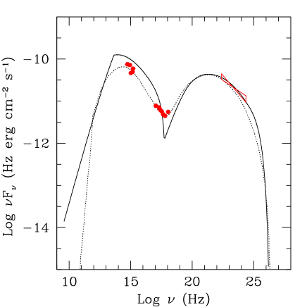
Figure 1: Model spectrum using parameters for 1749+096 (z=0.322) from Ghisellini et al (2010) (solid black line). Dotted line shows their spectrum for the same parameters and red points show their data.

4 Transition from High Frequency Peaked to Low Frequency Peaked BL Lacs with Accretion Rate

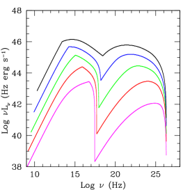
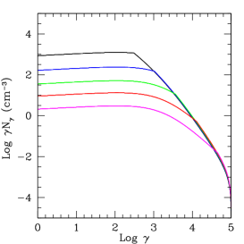
Figure 2: a). BL Lac model SEDs for fixed black hole mass and increasing accretion rate ($\dot{m}=10^{-4}$ (magenta), $3\times 10^{-4}$ (red), $10^{-3}$ (green), $3\times 10^{-3}$ (blue) and $10^{-2}$ (black), $M_{BH}=10^{8}M_{\odot}$). b). Corresponding steady state electron distributions. c). Fermi flux as a function of accretion rate, using mass and distance of model spectrum.

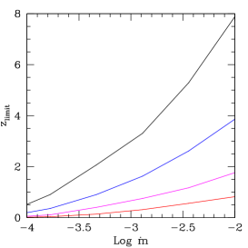
Figure 3: a). Decrease in observed flux with increasing viewing angle, where $\theta$ is measured in radians from the jet axis, for $\Gamma=15$. b). Redshift limits for Fermi visible BL Lacs as a function of black hole mass, for increasing viewing angle and $\dot{m}=10^{-2}$. c). Redshift limits for Fermi visible BL Lacs as a function of accretion rate, for $M_{BH}=10^{7}$ (red), $10^{8}$ (magenta), $10^{9}$ (blue) and $10^{10}M_{\odot}$ (black) and $\theta=0$.

We limit our model to a maximum accretion rate of $\dot{m}=10^{-2}$, since above this the accretion flow is expected to make a transition to a radiatively efficient thin disc. The strong UV and consequent broad line region emission provide additional seed photons, switching the main Fermi radiation process from SSC (BL Lacs) to EC (FSRQs).

Fig 2a shows a sequence of spectra with $R$, $P_{rel}$ and $B$ scaling as described above for $\dot{m}=10^{-2}$ (black) - $10^{-4}$ (magenta) for constant mass. This shows the systematic decrease in luminosity, coupled to a change in spectral shape from a low synchrotron peak energy (optical: LBL) to a high synchrotron peak energy (X-ray: HBL) as shown by Ghisellini & Tavecchio (2008; 2009).

We can compare the Fermi flux levels of our lower accretion rate spectra with observed HBLs. The HBL 1959+650 (see Tavecchio et al 2010 for a spectrum, G10 for spectral fitting parameters) has a mass of $2\times 10^{8}M_{\odot}$, so only slightly larger than the $10^{8}M_{\odot}$ system shown in Fig 2a. 1959+650 has an injected $P_{rel}$ of $7\times 10^{40}ergs^{-1}$ (G10), corresponding in our scalings to $\dot{m}=2.45\times 10^{-4}$. So it should have a similar Fermi flux to the red spectrum of fig 2a, which corresponds to $\dot{m}=3\times 10^{-4}$, $M=10^{8}$. The observed $\log(\nu L(\nu))$ Fermi flux of 1959+650 at $10^{23}Hz$ is $~{}43.5Hzergs^{-1}$, which is consistent with our red spectrum.

The changing shape of the emitted spectrum with accretion rate is due to the decrease in seed photons for electron cooling at lower $\dot{m}$, as shown explicitly by the the corresponding self consistent electron distributions in Fig 2b. The Lorentz factor of electrons which can cool in a light crossing time is $\gamma_{cool}\propto 1/(RU_{seed})\propto(1/M)(M/\dot{m})\propto 1/\dot{m}$. The lowest mass accretion rate ($\dot{m}=10^{-4}$, magenta) shows cooling only for the highest Lorentz factors, with $\gamma_{cool}\sim 10^{4.5}$. Below this the shape of the electron distribution is the same as the injected distribution, with a smooth break at $\gamma_{b}\sim 10^{3}$. As $\dot{m}$ increases, the sharp break at $\gamma_{cool}$ moves to lower Lorentz factors. For the black electron distribution corresponding to $\dot{m}=10^{-2}$, $\gamma_{cool}$ is comparable to $\gamma_{b}$. This is clear from the black spectrum in Fig 2a, where the spectral peak is now produced by the cooled electron distribution above $\gamma_{cool}$.

Increasing cooling, as a result of increasing accretion rate, therefore provides a natural explanation for the existence of high frequency peaked (HBL) and low frequency peaked (LBL) BL Lacs (Ghisellini & Tavecchio 2008; 2009). In the context of our model, HBLs correspond to black holes with very low accretion rates. There is very little cooling and the bulk of the synchrotron emission is produced by electrons with Lorentz factors close to $\gamma_{max}$. Their electron distributions most closely resemble the original injected distributions. LBLs correspond to black holes with higher accretion rates, where cooling becomes increasingly important and the bulk of the energy is produced by electrons close to $\gamma_{cool}$.

Since HBLs are at lower accretion rates they are intrinsically fainter and so should be observed at lower redshifts than LBLs. This is indeed observed (Shaw et al 2013). Fermi sensitivity is also a strong function of spectral index, decreasing with spectral hardness (Nolan et al 2012). Since LBLs have softer spectra this suggests Fermi will preferentially select LBLs over HBLs due to spectral shape as well as flux.

Fig 2a also shows that as $\dot{m}$ increases, the ratio of the Compton to synchrotron luminosities changes. With our scalings, $L_{sync}\propto R^{3}U_{B}K$ and $L_{comp}\propto R^{3}U_{sync}K\propto R^{3}(RU_{B}K)K$, ie. $L_{sync}/L_{comp}\propto 1/(RK)$, where $K$ is the normalisation of the steady state electron distribution. If there is complete cooling, ie. $\gamma_{cool}<\gamma_{min}$, then $K\propto Q_{0}/U_{seed}\propto(\dot{m}/M^{2})(\dot{m}/M)^{-1}\propto 1/M$ which is independent of accretion rate. However the BL Lac spectra do not show complete cooling (see Fig 2b). If there is no cooling, $K\sim RQ_{0}/c\propto\dot{m}/M$. The BL Lac spectra lie in this regime where the cooling is incomplete, hence $L_{sync}/L_{comp}\propto 1/\dot{m}$. This can be seen in Fig 2b, where the normalisation of the electron distribution at $\gamma=1$ increases with $\dot{m}$. The scaling is not exactly $K\propto\dot{m}$, since there is an additional dependence on $\dot{m}$ introduced by $\gamma_{cool}$ decreasing through the intermediate regime.

Fig 2c shows how the flux in the Fermi band drops with accretion rate. For higher accretion rates, cooling is efficient, so $L_{comp}\propto\dot{m}$. For low accretion rates, cooling is inefficient so $L_{comp}\propto\dot{m}^{3}$.

However, a more detailed comparison of Fig 2a to the data in the ’blazar sequence’ shows evidence that the Compton flux changes more slowly with decreasing mass accretion rate due to an increase in the maximum Lorentz factor of the accelerated electron distribution (Ghisellini & Tavecchio 2008; 2009). Again, this can be a consequence of the different cooling environment, where electrons are accelerated to a maximum energy which is set by a balance between the acceleration timescale and the cooling timescale. Thus the accelerated electron distribution may itself change with cooling, such that $\gamma_{b}\propto\gamma_{max}\propto 1/U_{seed}$. We will consider such models later in the paper.

5 BL Lac Visibility

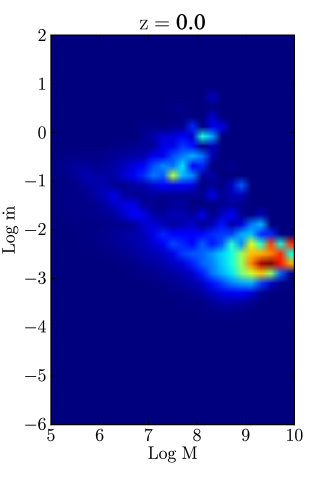
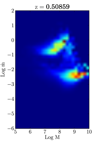
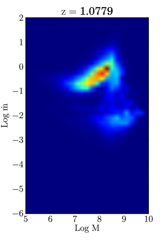
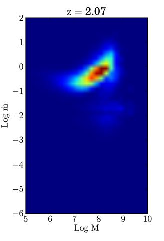
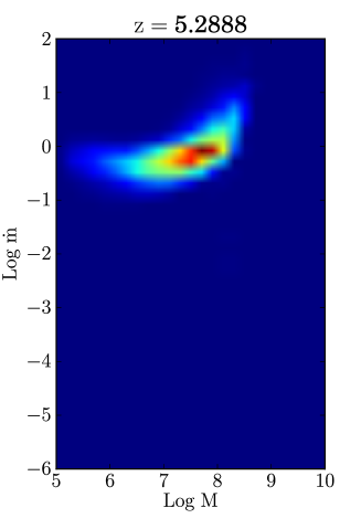
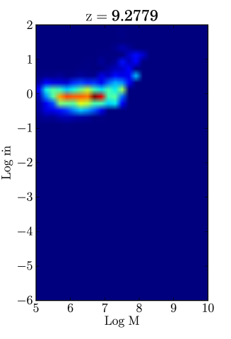
Figure 4: Predicted mass and accretion rate distribution of accreting black holes at increasing redshift from Millennium simulation. Colours trace luminosity density, with red showing the mass and accretion rates at which the maximum accretion luminosity is emitted at each redshift.

The visibility of a BL Lac is strongly affected by viewing angle. Fig 3a shoes how sharply the observed luminosity decreases for our assumed $\Gamma=15$ with increasing viewing angle, where $\theta$ is measured in radians from the jet axis. Thus there is a difference of $10^{12}$ between the observed flux from a face on jet compared to an edge on jet.

The more distant the source, the more closely aligned to our line of sight the jet must be in order to boost the observed flux to a visible level. We define a flux limit of $F_{100MeV-100GeV}>5\times 10^{-12}ergs^{-1}cm^{-2}$ from the Fermi 2 year catalogue (Nolan et al 2012), and show in Fig 3b the limiting redshift, $z_{limit}$, at which a BL Lac at $\dot{m}=10^{-2}$ with different masses can be detected by Fermi at different inclination angles. We include the effects of absorption from pair production on the extragalactic IR background using the model of Kneiske & Dole (2010), though this is negligible. Only the most massive black holes, $\sim 10^{10}M_{\odot}$ which are most closely aligned to our line of sight can be seen out beyond $z=4$. $z_{limit}$ drops by a factor of $\sim 3$ if the inclination angle is increased from $0$ to the more statistically likely $1/\Gamma$. This represents a change of just $\sim 4^{\circ}$ for $\Gamma=15$ used in our calculations. For a typical BL Lac mass of $10^{9}M_{\odot}$ viewed at $1/\Gamma$ the maximum observable redshift is $z\sim 1$, increasing to $4$ only for the most face on jets.

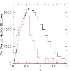
Figure 5: a). Predicted redshift distribution of Fermi visible BL Lacs, assuming BHs of all spins accreting below $\dot{m}=10^{-2}$ produce a BL Lac type jet (black). Red solid line shows observed redshift distribution of Fermi detected BL Lacs. Red dashed line shows observed redshift distribution $\times 100$. b). Predicted mass distribution of Fermi visible BL Lacs. c). Predicted accretion rate distribution of Fermi visible BL Lacs.

Fig 3c shows how the redshift limit drops as a function of accretion rate for each mass ($10^{10}$ (black), $10^{9}$ (blue), $10^{8}$ (magenta) and $10^{7}M_{\odot}$ (red)) black hole for $\theta=0$. If LBLs correspond to BL Lacs at $\dot{m}\sim 10^{-2}$ and HBLs at $\dot{m}<10^{-3}$ this shows how the redshift limits for the two populations should differ, with the majority of HBLs being observed below $z=3$. Shaw et al (2013) find this to be the case, with the distribution of LBLs extending to higher $z$, although they find the means of both populations are well below $z=3$.

6 Predicted BL Lac Population from Cosmological Simulations

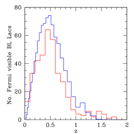
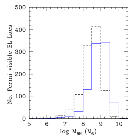
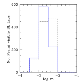
Figure 6: a). Predicted redshift distribution of Fermi visible BL Lacs, assuming only BHs with spins $a>0.8$ produce a BL Lac type jet (blue). Red solid line shows observed redshift distribution of Fermi detected BL Lacs. b). Predicted mass distribution including only BHs with $a>0.8$ (blue). Black dashed line shows predicted distribution including all BHs $\times 0.01$. c). Predicted accretion rate distribution including only BHs with $a>0.8$ (blue). Black dashed line shows predicted distribution including all BHs $\times 0.01$.

Cosmological simulations predict the number of supermassive black holes accreting at different redshifts, together with their masses and accretion rates. These simulations have been found to agree well with the observed number densities of broad line and narrow line AGN in the local universe (Fanidakis et al 2011; 2012). Combining our spectral code with the black hole data from these simulations allows us to predict the number of AGN that should be detected as BL Lacs by Fermi.

We combine our code with the black hole number densities predicted by the Millennium Simulation (Springel et al 2005; Fanidakis et al 2011; 2012), binned as a function of both mass and mass accretion rate. We define a luminosity density from the number density multiplied by the luminosity at that mass and mass accretion rate i.e. $L=\eta\dot{M}c^{2}$ for the thin disc regime $10^{-2}<\dot{m}<1$, joining smoothly onto a radiatively inefficient regime at lower $\dot{m}$ where $L\propto\dot{m}^{2}$ (Narayan & Yi 1995) and onto a super-Eddington flow at higher $\dot{m}$ where $L\propto\ln(1+\dot{m})$ (Shakura & Sunyaev 1973). The luminosity density in each $(z,M,\dot{m})$ bin therefore depends on the mass, accretion rate, spin (which sets $\eta$), the inferred accretion regime and the number of black holes in that bin.

Fig 4 shows the evolution of the luminosity density of accretion power across cosmic time showing the features described by Fanidakis et al (2011; 2012). At high redshift there is plenty of gas to fuel accretion. The black holes accrete close to the Eddington limit and grow rapidly. Comparing the snapshots for $z\sim 9$ and $z\sim 5$, the typical black hole mass producing the bulk of the accretion luminosity increases from $\sim 10^{6}$ to $\sim 10^{8}M_{\odot}$. As the black holes gradually run out of gas, their accretion rates drop (compare $z\sim 2$ and $z\sim 1$). By redshift 2, accretion rates are beginning to drop below $\dot{m}=10^{-2}$, into the regime at which BL Lac type jets should be produced. This suggests no BL Lacs should be observed much above $z\sim 2$, not just because the flux becomes too faint, but because the typical accretion rate is too high for the production of BL Lac jets.

We select only black holes in the radiatively inefficient regime ($\dot{m}<10^{-2}$), assuming all BHs accreting inefficiently will produce a BL Lac type jet, and calculate the number of AGN hosting a BL Lac type jet in each $(z,M,\dot{m})$ bin. If this number is less than 1 we use Poisson statistics to randomly determine whether a BH is present or not. Each black hole in each $(z,M,\dot{m})$ bin is then assigned a random distance within this redshift bin and random $\theta_{obs}$, assuming $\cos\theta_{obs}$ is distributed uniformly. We then calculate the observed spectrum to determine whether or not the jet would be visible to Fermi.

Fig 5a shows the predicted redshift distribution of Fermi visible BL Lacs (black). The predicted distribution peaks at $z\sim 0.5$ and drops gradually to $z\sim 2$. No BL Lacs are observed above this point, not because they are not visible (see Fig 3b), but because there simply are not enough SMBHs accreting below $10^{-2}$ in the cosmological simulations to produce SSC jets, due to the higher activity expected at earlier times. The low redshift distribution of BL Lacs is a direct result of cosmic downsizing and the requirement of an $\dot{m}<10^{-2}$ to produce a SSC jet.

However, comparing this to observations shows a huge discrepancy (red solid line from Shaw et al 2013, which almost merges with the X-axis at this scale). Our expected number of $\sim 100000$ BL Lacs dramatically overpredicts the observed number of Fermi detections ($\sim 500$). A clear illustration of the problem can be seen from simply the number density of massive ($8<\log M<9$) black hole accretion flows with $10^{-3}<\dot{M}<10^{-2}$ in the cosmological simulations in the redshift bin centred around $z\sim 0.5$ (Fanidakis et al 2011). This number is $6.8\times 10^{-4}Mpc^{-3}$ and the volume of this bin, from $0.509<z<0.564$ is $\sim 9$ Gpc³ so this gives $6101659$ objects which should host similar jets to 1749+096 (Fig 1), i.e. have Fermi flux of $10^{-10.5}(0.5/0.322)^{-2}\sim 10^{-11}$ ergs cm^-2 s^-1 if viewed at the same angle (roughly $1/\Gamma$). The probability that we see the source within this angle is $1-\cos(1/\Gamma)$, so the expected number of Fermi detections of these sources alone is $\approx 13554$, similar to the full calculation results. The large discrepancy clearly points to a fundamental breakdown of one of the assumptions.

On a more subtle level, the shape of the redshift distribution for the Fermi predictions is also mismatched to the observations. The red dashed line shows the observed number of BL Lacs scaled by a factor of 100 so it can be compared to the predicted distribution. We define redshift from Shaw et al (2013) as either spectroscopic redshift, spectroscopic lower limit, the mean of their redshifts derived from host galaxy fitting, or their redshift upper limits, in that order of preference. The dashed line shows this observed redshift distribution ($\times 100$). It is clear that not only is the total predicted number wrong, but we are also over estimating the proportion of BL Lacs in the range $z=0.5-2$.

The mass distribution and mass accretion rate distributions are as expected (Figs 5b and c), with higher luminosity SSC flows (i.e. higher $\dot{m}M$) being more likely to be observed, so simple energetics selects the highest mass and mass accretion rate objects, so the typical predicted mass of a Fermi visible BL Lac $\sim 10^{8.5}-10^{9}M_{\odot}$ is a combination of three factors:

1. Very few black holes accreting at $\dot{m}<10^{-2}$ above $z=2$.

2. Most black holes at $z<2$ accreting with $\dot{m}<10^{-2}$ have $M>10^{8}$.

3. Black holes with $M>10^{9}$ are increasingly rare in the local universe so we are less likely to observe one favourably orientated to our line of sight.

7 Another Factor Affecting Jet Scaling?

Our results predict $\sim 10^{5}$ BL Lacs should have been detected in the Fermi 2 year catalogue. In contrast, $\sim 500$ objects in the 2nd Fermi LAT catalogue are classed as BL Lacs. Even allowing for galactic centre emission limiting sky coverage ($|b|>10^{\circ}$ means that only 80% of the sky is included), this is still 3 orders of magnitude larger than observed. Clearly jets do not simply scale with accretion power.

We assumed the injected electron distribution was independent of mass accretion rate. This may not be the case. Ghisellini & Tavecchio (2009) approximately use $\gamma_{max}\propto\gamma_{b}\propto 1/\dot{m}$ to fit their blazar sequence. Acceleration of electrons is affected by the ambient photon field which depends on the amount of cooling and ultimately on accretion rate. In the efficient cooling regime, $L_{sync}\propto L_{comp}\propto\dot{m}M$, making $\gamma_{max}\propto 1/\dot{m}$ not unreasonable. However, an increase of $\gamma_{max}$, and $\gamma_{b}$ in particular, only serves to increase the Fermi band luminosity for lower $\dot{m}$ systems, and increase the discrepancy between the predictions and observations.

The discrepancy could instead be explained if every BH accreting below $10^{-2}$ has the potential to produce a BL Lac type jet, but only does so $1/1000th$ of the time. This seems unlikely, since Fanaroff Riley Type I (FRI) AGN, the misaligned versions of BL Lacs (Padovani & Urry 1990, Padovani & Urry 1991, Urry, Padovani & Stickel 1991) show large scale extended radio jets. This suggests these jets are persistent, analogous to the steady low/hard state jet seen in BHBs at low $\dot{m}$, not transient events.

Another possibility is that the jet depends on magnetic flux being advected onto the black hole from the extremely large scale hot halo gas around the galaxy. Sikora & Begelman (2013) suggest that if there is magnetic flux in this gas, then it could be dragged down close to the black hole by cold gas from a merging spiral galaxy. However, this does not address the fundamental question as to where the magnetic flux in the halo gas comes from, and using cold gas from a spiral merger to drag this field down to the black hole is unlikely to be applicable in the BL Lacs as they have low ongoing mass accretion rates.

The bulk Lorentz factor of the jet is the biggest factor affecting its visibility. We rerun our calculations with a reduced $\Gamma=10$ instead of 15 and find this roughly halves the predicted number of BL Lacs, but still wildly overpredicts the observations.

We have assumed all jets are produced with the same value of bulk Lorentz factor but this is clearly not the case - BHBs at low $\dot{m}$ have $\Gamma\sim 1.2$ (Fender et al 2004). The most obvious way to reduce the number of visible BL Lacs is to allow a distribution of $\Gamma$. Yet there must be some physical parameter which controls the jet acceleration. The acceleration region, where the magnetic (Poynting) flux of the jet is converted to kinetic energy, is very close to the black hole, so it seems most likely that this is set by the black hole itself, in which case black hole spin is the only remaining plausible parameter. A potential explanation for the lower number of observed BL Lacs is that if only BHs with the highest spin produce highly relativistic jets, and high spin is rare.

The cosmological simulations include the growth of SMBH spin via accretion processes and black hole-black hole coalescence following galaxy mergers (Volonteri et al 2005; 2007; 2012: Fanidakis et al 2011; 2012). The mass accumulated onto the central SMBH in an accretion event is tied in the simulation to a fixed fraction (0.5%) of the mass of gas in a star formation episode in the host galaxy. If this mass is all accreted in a single event (prolonged accretion) then this is sufficient to spin most black holes up to maximal (Volonteri et al 2005; 2007). However, the mass accreting onto the central black hole in any single event may be limited by self gravity. This splits the accreting material up into multiple smaller events, each of which can be randomly aligned since the star formation scale height is large compared to the black hole sphere of influence even in a disc galaxy (King et al 2008). Such chaotic accretion flow models result in predominantly low spin black holes (Volonteri et al 2007: King et al 2008: Fanidakis et al 2011; 2012), and high spins are rare as they are produced not via accretion but via black hole mergers (Fanidakis et al 2011; 2012).

We use the spin distribution from the chaotic accretion flow model simulations, and introduce a spin cut to our results, so that only BHs with spin greater than $a_{cut}\sim 0.8$ produce a BL Lac type jet. This reduces the predicted number of Fermi visible BL Lacs to $\sim 900$. Fig 6a shows the resulting redshift distribution together with the observed distribution. Not only does this reduce the discrepancy between predicted and observed total numbers, it also gives a better match to the shape of the distribution. Limiting production of BL Lac type jets to BHs with high spin causes the redshift distribution to peak slightly later and drop off more sharply above $z=0.5$. This is because high spins arise from BH mergers. Production of BL Lac jets is already limited to BHs accreting below $10^{-2}$, ie. $M>10^{8}$. The BH mergers which make the most massive BHs occurs at the latest times.

Fig 6b and 6c show how this affects the predicted mass and accretion rate distributions of Fermi visible BL Lacs. The scaled down distributions including BHs of all spins are shown by the dashed lines for comparison. Requiring high spin increases the peak of the mass distribution to $\sim 10^{8.5}-10^{9.5}$, because it is the most massive BHs that are former by mergers and are consequently more likely to have high spin. The peak of the accretion rate distribution is actually slightly reduced. This is because the more massive BHs have lower accretion rates; the spin cut has excluded lower mass BHs with lower spins which tend to have slightly higher accretion rates.

The low spin, low accretion rate BHs, which generally have smaller masses ($10^{7}-10^{8}M_{\odot}$) correspond to the LINERs, which are not observed to have jets as relativistic as those in BL Lacs. If they are low spin, as expected, and high spin is required for a highly relativistic jet, then this naturally explains why LINERs are observed to have weaker radio jets.

8 Implications of Scaling Jet Power with Spin: FRI Sources

The parent population of BL Lacs is probably the Fanaroff Riley Type I (FRI) sources (e.g. the review by Urry & Padovani 1995). These show ’fluffy’ radio jets whose surface brightness decreases with distance from the central source, contrasting with the classic lobe and hotspot radio emission seen in the more powerful FRII sources which are the parent population of the FSRQ (Padovani & Urry 1992). Thus the FRI sources should also correspond to high spin BHs, and indeed are similarly powered by high mass SMBHs (Woo & Urry 2002).

However, we might then expect some difference in jet radio emission between the FRIs and lower mass LINERs as the cosmological simulations predict that the lower mass SMBHs have lower spin (Fanidakis et al 2011; 2012). Sikora et al (2007) claim that this difference is indeed seen, with radio emission being $\sim 3$ orders of magnitude higher in the FRIs.

However, some of this difference disappears when only core radio luminosity (rather than core plus lobes) is used (Broderick & Fender 2011). This is clearly an issue as the extended radio emission must depend on environment. The BHs in FRIs are more massive than those in LINERs, hence live in richer cluster environments, with larger dark matter halos which trap more hot cluster gas. The jet then emerges into a denser, higher pressure environment, which means that a much larger fraction (potentially all) of the jet kinetic energy is converted to radiation and/or heating of the cluster gas (Birzan et al 2004). Conversely, any jet from the lower mass LINERs emerges into a poorer group environment, so adiabatic losses can predominate and the extended radio emission is much smaller (e.g. Krause et al 2012).

Some of the remaining difference in core radio power is expected due to the difference in mass (Broderick & Fender 2011). However, even accounting for this there is still a factor of $\sim 10$ in mass corrected, core radio emission. The LINERs lie on the Fundamental plane (Merloni et al 2003; Falcke et al 2004) i.e. have the expected core radio emission for their black hole mass and mass accretion rate, so the FRIs are a factor 10 brighter in mass corrected, core radio emission than expected from the same jet models which produce the low bulk Lorentz factor BHB and LINER jets, consistent with the idea that the jet is intrinsically more powerful/has higher Lorentz factor due to black hole spin.

It is difficult to predict the difference in core radio emission with black hole spin in our models as synchrotron self-absorption means that the observed radio emission does not arise in the same region as produces the Fermi flux. It may be produced either at larger radii, perhaps where the jet has decelerated, or in a lower density, lower bulk Lorentz factor layer surrounding the $\Gamma=15$ spine of the jet. Either of these could explain the lower Lorentz factor ($\Gamma\sim 2-10$) of the radio jet observed in FRIs (Chiaberge et al 2000), though the spine-layer structure may additionally be able to explain the very fast variability timescales seen in some BL Lacs (Ghisellini & Tavecchio 2008).

9 Conclusions

We have taken a statistical approach to constrain the conditions necessary to produce the highly relativistic jets seen in BL Lac objects. We combine SMBH number densities from cosmological simulations, known to reproduce the optical luminosity function of AGN, with spectral models of jet emission and simple jet scaling functions which depend only on mass and accretion rate. The key assumption is that every BH accreting with $\dot{m}<10^{-2}$ i.e. in the radiatively inefficient accretion flow regime, should produce a BL Lac type jet.

Our calculation of the expected number of BL Lacs detectable by Fermi overpredicts the observations by three orders of magnitude. This clearly shows that our fundamental assumptions are incorrect, and that the jet power and properties do not scale simply with mass and mass accretion rate. The only other parameter which a black hole can have is spin. We can reproduce the observed numbers of BL Lacs if SMBHs grow predominantly via chaotic (randomly aligned) accretion episodes, and that BL Lac type jets are restricted to BHs with spin $a>0.8$. These are rare as they form from BH-BH coalescence following a major merger event which is not then overwhelmed by further chaotic accretion i.e. this requires a gas poor major merger event, and only the most massive galaxies, which host the most massive black holes, are gas poor in the local Universe (Fanidakis et al 2011; 2012).

A spin cut is in line with the longstanding speculation that these most relativistic jets require high spin black holes (Maraschi et al 2012), and also gives a good match to the observed redshift distribution of BL Lacs which peaks at $z=0.5$ and then drops off sharply, with no objects above $z\sim 2$. This is a consequence of three factors:

1. BL Lac jets are restricted to BHs with $\dot{m}<10^{-2}$, and there are no BHs accreting at $\dot{m}<10^{-2}$ above $z\sim 2$.

2. Only the most massive BHs have high spin through mergers, which happen at late times, causing the bulk of the population to fall below $z=1$

3. These most massive objects are rare in the local universe causing the distribution to decrease again below $z=0.5$.

Since FRI sources are consistent with being the misaligned analogs of BL Lacs, they should also have high spin. They are indeed offset from the Fundamental Plane, i.e. have higher (mass corrected) core radio emission to the lower mass and presumably lower spin LINERs, though only by a factor $\sim 10$ (Broderick & Fender 2011). However, the radio emission is not predominantly produced from the same region as the Fermi flux so may not be as sensitive to the difference in spin.

10 Acknowledgements

We thank Nikos Fanidakis and the Millennium simulation for use of their data. This work has made use of Ned Wright’s Cosmology Calculator (Wright 2006). EG acknowledges funding from the UK STFC.

Appendix A

The emission comes from a single zone of radius $R$. We assume material in the jet moves at a constant bulk Lorentz factor ($\Gamma$) and that some fraction of the transported electrons are accelerated into a power law distribution between minimum and maximum Lorentz factors $\gamma_{min}$ and $\gamma_{max}$, of the form:

$$Q(\gamma)=Q_{0}\left(\frac{\gamma}{\gamma_{b}}\right)^{-n_{1}}\left(1+\gamma/\gamma_{b}\right)^{n1-n2}=Q_{0}q(\gamma)\\ \mbox{ for }\gamma_{min}<\gamma<\gamma_{max}$$ (6)

$\gamma_{b}$ is the Lorentz factor at which the electron distribution changes in slope from $n_{1}$ to $n_{2}$. We calculate the normalisation $Q_{0}$ from the power injected into the accelerated electrons ($P_{rel}$):

$$P_{rel}=\frac{4\pi}{3}R^{3}m_{e}c^{2}Q_{0}\int_{\gamma_{min,inj}}^{\gamma_{max}}\gamma q(\gamma)d\gamma$$ (7)

We calculate $\gamma_{cool}$ after a light crossing time $t_{cross}=R/c=\gamma_{cool}/\dot{\gamma}_{cool}$, as:

$$\gamma_{cool}=\frac{3m_{e}c^{2}}{4\sigma_{T}RU_{seed}}$$ (8)

Where $U_{seed}=U_{B}+U_{sync}$ is the sum of the energy density in magnetic fields and synchrotron emission which provides the seed photons for cooling.

We solve the continuity equation to find the self consistent steady state electron distribution:

$$\begin{split}N(\gamma,t_{cross})&=Kn(\gamma)\\ &=\begin{cases}AQ_{0}q(\gamma)\\ &\mbox{ for }\gamma_{min}<\gamma<\gamma_{cool}\\ \frac{3m_{e}c^{2}}{4\sigma_{T}cU_{seed}}\frac{Q_{0}}{\gamma^{2}}\int_{\gamma}^{\gamma_{max}}q(\gamma)d\gamma\\ &\mbox{ for }\gamma_{cool}<\gamma<\gamma_{max}\end{cases}\end{split}$$ (9)

Where $A$ is found by matching at $\gamma_{cool}$.

We use the delta function approximation and calculate the synchrotron emissivity as:

$$j_{sync}(\nu)=\frac{\sigma_{T}c}{6\pi\nu_{B}}U_{B}\gamma N(\gamma)$$ (10)

Where the electron Lorentz factor and synchrotron photon frequency are related by $\gamma=\sqrt{3\nu/4\nu_{B}}$ and we calculate the synchrotron self-absorption frequency ($\nu_{ssa}$) as given by (Ghisellini et al. 1985):

$$\nu_{ssa}=\left(4.62\times 10^{14}KB^{2.5}\frac{R_{j}}{0.7}\right)^{2/7}$$ (11)

We calculate synchrotron self-Compton emission including the Klein-Nishina cross section using the delta approximation:

$$j_{comp}(\nu)=\frac{\sigma_{T}c}{6\pi}\int^{\gamma_{max}}_{\gamma_{min}}\int^{\nu_{sync,max}}_{\nu_{ssa}}\frac{U_{sync}(\nu_{sync})}{\nu_{sync}}\gamma N(\gamma)d\nu_{sync}d\gamma$$ (12)

Where electron Lorentz factor and Compton photon frequency are related by $\gamma=\sqrt{3\nu/4\nu_{sync}}$.

Bulk motion of the jet boosts and blue shifts the emission. We calculate the observed flux as:

$$F(\nu\delta/(1+z))=\frac{(j_{sync}(\nu)+j_{comp}(\nu))}{R_{co}^{2}}\frac{4\pi}{3}R^{3}\delta^{3}$$ (13)

Where $\delta=(\Gamma-\cos{\theta}\sqrt{\Gamma^{2}-1})^{-1}$ is the Doppler factor and $R_{co}$ is the comoving distance to the object at redshift $z$.

References

- [\citeauthoryearBest & Heckman2012] Best P. N., Heckman T. M., 2012, MNRAS, 421, 1569
- [\citeauthoryearBîrzan et al.2004] Bîrzan L., Rafferty D. A., McNamara B. R., Wise M. W., Nulsen P. E. J., 2004, ApJ, 607, 800
- [\citeauthoryearBlandford & Znajek1977] Blandford R. D., Znajek R. L., 1977, MNRAS, 179, 433
- [\citeauthoryearBlandford & Payne1982] Blandford R. D., Payne D. G., 1982, MNRAS, 199, 883
- [\citeauthoryearBroderick & Fender2011] Broderick J. W., Fender R. P., 2011, MNRAS, 417, 184
- [\citeauthoryearChiaberge et al.2000] Chiaberge M., Celotti A., Capetti A., Ghisellini G., 2000, A&A, 358, 104
- [\citeauthoryearCzerny & Hryniewicz2012] Czerny B., Hryniewicz K., 2012, JPhCS, 372, 012013
- [\citeauthoryearDermer, Schlickeiser, & Mastichiadis1992] Dermer C. D., Schlickeiser R., Mastichiadis A., 1992, A&A, 256, L27 Dermer, C.D., & Mernon, M. 2009, High Energy Radiation from Black Holes: Gamma Rays, Cosmic Rays, and Neutrinos, Princeton University Press,
- [\citeauthoryearDone, Gierliński, & Kubota2007] Done C., Gierliński M., Kubota A., 2007, A&ARv, 15, 1
- [\citeauthoryearEsin, McClintock, & Narayan1997] Esin A. A., McClintock J. E., Narayan R., 1997, ApJ, 489, 865
- [\citeauthoryearFalcke1996] Falcke H., 1996, ApJ, 464, L67
- [\citeauthoryearFalcke & Markoff2000] Falcke H., Markoff S., 2000, A&A, 362, 113
- [\citeauthoryearFalcke, Körding, & Markoff2004] Falcke H., Körding E., Markoff S., 2004, A&A, 414, 895
- [\citeauthoryearFanidakis et al.2011] Fanidakis N., Baugh C. M., Benson A. J., Bower R. G., Cole S., Done C., Frenk C. S., 2011, MNRAS, 410, 53
- [\citeauthoryearFanidakis et al.2012] Fanidakis N., et al., 2012, MNRAS, 419, 2797
- [\citeauthoryearFender, Belloni, & Gallo2004] Fender R. P., Belloni T. M., Gallo E., 2004, MNRAS, 355, 1105
- [\citeauthoryearFossati et al.1998] Fossati G., Maraschi L., Celotti A., Comastri A., Ghisellini G., 1998, MNRAS, 299, 433
- [\citeauthoryearGhisellini, Maraschi, & Treves1985] Ghisellini G., Maraschi L., Treves A., 1985, A&A, 146, 204
- [\citeauthoryearGhisellini et al.1998] Ghisellini G., Celotti A., Fossati G., Maraschi L., Comastri A., 1998, MNRAS, 301, 451
- [\citeauthoryearGhisellini, Tavecchio, & Chiaberge2005] Ghisellini G., Tavecchio F., Chiaberge M., 2005, A&A, 432, 401
- [\citeauthoryearGhisellini & Tavecchio2008] Ghisellini G., Tavecchio F., 2008, MNRAS, 387, 1669
- [\citeauthoryearGhisellini & Tavecchio2008] Ghisellini G., Tavecchio F., 2008, MNRAS, 386, L28
- [\citeauthoryearGhisellini & Tavecchio2009] Ghisellini G., Tavecchio F., 2009, MNRAS, 397, 985
- [\citeauthoryearGhisellini, Maraschi, & Tavecchio2009] Ghisellini G., Maraschi L., Tavecchio F., 2009, MNRAS, 396, L105
- [\citeauthoryearGhisellini et al.2010] Ghisellini G., Tavecchio F., Foschini L., Ghirlanda G., Maraschi L., Celotti A., 2010, MNRAS, 402, 497
- [\citeauthoryearGhisellini et al.2011] Ghisellini G., Tavecchio F., Foschini L., Ghirlanda G., 2011, MNRAS, 414, 2674
- [\citeauthoryearHeinz & Sunyaev2003] Heinz S., Sunyaev R. A., 2003, MNRAS, 343, L59
- [\citeauthoryearHeinz2004] Heinz S., 2004, MNRAS, 355, 835
- [\citeauthoryearKing, Pringle, & Hofmann2008] King A. R., Pringle J. E., Hofmann J. A., 2008, MNRAS, 385, 1621
- [\citeauthoryearKneiske & Dole2010] Kneiske T. M., Dole H., 2010, A&A, 515, A19
- [\citeauthoryearKrause et al.2012] Krause M., Alexander P., Riley J., Hopton D., 2012, MNRAS, 427, 3196
- [\citeauthoryearMahadevan1997] Mahadevan R., 1997, ApJ, 477, 585
- [\citeauthoryearMaraschi et al.2012] Maraschi L., Colpi M., Ghisellini G., Perego A., Tavecchio F., 2012, JPhCS, 355, 012016
- [\citeauthoryearMaraschi & Tavecchio2003] Maraschi L., Tavecchio F., 2003, ApJ, 593, 667
- [\citeauthoryearMartínez-Sansigre & Rawlings2011] Martínez-Sansigre A., Rawlings S., 2011, MNRAS, 414, 1937
- [\citeauthoryearMerloni, Heinz, & di Matteo2003] Merloni A., Heinz S., di Matteo T., 2003, MNRAS, 345, 1057
- [\citeauthoryearMurray & Chiang1997] Murray N., Chiang J., 1997, ApJ, 474, 91
- [\citeauthoryearNarayan & Yi1995] Narayan R., Yi I., 1995, ApJ, 452, 710
- [\citeauthoryearNarayan & McClintock2012] Narayan R., McClintock J. E., 2012, MNRAS, 419, L69
- [\citeauthoryearNolan et al.2012] Nolan P. L., et al., 2012, ApJS, 199, 31
- [\citeauthoryearPadovani & Urry1990] Padovani P., Urry C. M., 1990, ApJ, 356, 75
- [\citeauthoryearPadovani & Urry1991] Padovani P., Urry C. M., 1991, ApJ, 368, 373
- [\citeauthoryearPadovani & Urry1992] Padovani P., Urry C. M., 1992, ApJ, 387, 449
- [\citeauthoryearRussell, Gallo, & Fender2013] Russell D. M., Gallo E., Fender R. P., 2013, MNRAS, 431, 405
- [\citeauthoryearSatyapal et al.2005] Satyapal S., Dudik R. P., O’Halloran B., Gliozzi M., 2005, ApJ, 633, 86
- [\citeauthoryearShakura & Sunyaev1973] Shakura N. I., Sunyaev R. A., 1973, A&A, 24, 337
- [\citeauthoryearShaw et al.2013] Shaw M. S., et al., 2013, ApJ, 764, 135
- [\citeauthoryearSikora, Begelman, & Rees1994] Sikora M., Begelman M. C., Rees M. J., 1994, ApJ, 421, 153
- [\citeauthoryearSikora, Stawarz, & Lasota2007] Sikora M., Stawarz Ł., Lasota J.-P., 2007, ApJ, 658, 815
- [\citeauthoryearSikora & Begelman2013] Sikora M., Begelman M. C., 2013, ApJ, 764, L24
- [\citeauthoryearSpringel et al.2005] Springel V., et al., 2005, Natur, 435, 629
- [\citeauthoryearTavecchio et al.2010] Tavecchio F., Ghisellini G., Ghirlanda G., Foschini L., Maraschi L., 2010, MNRAS, 401, 1570
- [\citeauthoryearUrry, Padovani, & Stickel1991] Urry C. M., Padovani P., Stickel M., 1991, ApJ, 382, 501
- [\citeauthoryearUrry & Padovani1995] Urry C. M., Padovani P., 1995, PASP, 107, 803
- [\citeauthoryearVolonteri et al.2005] Volonteri M., Madau P., Quataert E., Rees M. J., 2005, ApJ, 620, 69
- [\citeauthoryearVolonteri, Sikora, & Lasota2007] Volonteri M., Sikora M., Lasota J.-P., 2007, ApJ, 667, 704
- [\citeauthoryearVolonteri2012] Volonteri M., 2012, Sci, 337, 544
- [\citeauthoryearWoo & Urry2002] Woo J.-H., Urry C. M., 2002, ApJ, 579, 530
- [\citeauthoryearWright2006] Wright E. L., 2006, PASP, 118, 1711