Ranking Algorithms by Performance

Abstract

A common way of doing algorithm selection is to train a machine learning model and predict the best algorithm from a portfolio to solve a particular problem. While this method has been highly successful, choosing only a single algorithm has inherent limitations – if the choice was bad, no remedial action can be taken and parallelism cannot be exploited, to name but a few problems. In this paper, we investigate how to predict the ranking of the portfolio algorithms on a particular problem. This information can be used to choose the single best algorithm, but also to allocate resources to the algorithms according to their rank. We evaluate a range of approaches to predict the ranking of a set of algorithms on a problem. We furthermore introduce a framework for categorizing ranking predictions that allows to judge the expressiveness of the predictive output. Our experimental evaluation demonstrates on a range of data sets from the literature that it is beneficial to consider the relationship between algorithms when predicting rankings. We furthermore show that relatively naïve approaches deliver rankings of good quality already.

1 Introduction

The Algorithm Selection Problem [16] is to select the most appropriate algorithm for solving a particular problem. It is especially relevant in the context of algorithm portfolios [6, 3], where a single solver is replaced with a set of solvers and a mechanism for selecting a subset to use on a particular problem.

The most common approach to building such a selector is to use machine learning to induce a model of the algorithms in the portfolio. Such models can take many different shapes and forms. Common ones include classification or clustering approaches that select only a single solver to be run and regression approaches that predict the performance of each portfolio solver independently and choose one or several according to those predictions. While some of these approaches implicitly compute a ranking of the algorithms in the portfolio, almost none make explicit use of it.

In this paper, we investigate approaches that explicitly rank the portfolio algorithms according to their performance. Instead of predicting only the best algorithm, we compute a ranking over all of them. There are several advantages of this approach. Because we have information on all algorithms, we can use several or all of them for solving the problem or set of problems. If the algorithm that is chosen initially performs worse than expected, the next best can be chosen without having to make another prediction. If more than one processor is available, several can be run in parallel. This again limits the impact of bad predictions.

Several approaches in the literature, e.g. [14, 8], compute schedules for running the algorithms in the portfolio. Such schedules rely on a ranking of the algorithms that dictates when to run each algorithm and for how long. Despite this, no comparison of different ways of arriving at such a schedule has been performed to date.

While techniques that could also be used to derive a performance ranking of algorithms are abundant in the literature, very few researchers have investigated how and to what extent performance rankings can be predicted in practice. [11] shows that the prediction of the performance of target algorithms makes incorrect predictions very often and proposes a means of mitigating this, but again only for the best algorithm. This suggests that more sophisticated means for predicting complete rankings may be required.

In this paper, we propose and evaluate a range of different approaches, including ones that are commonly used in the literature for similar purposes, on data sets that we also take from the literature. Our evaluation fills a much-needed gap by addressing the issue of how one should predict complete performance rankings for algorithms in a portfolio context.

While a complete ranking is not required to do algorithm selection, it can be beneficial. Predictions of algorithm performance will always have some degree of uncertainty associated with them and being able to choose from among all portfolio algorithms in a meaningful way can be used to mitigate the effect of this. However, in order for this to be exploited, we must be able to predict the rankings to be used reliably and know what techniques are available for doing so. This is the core contribution of this paper.

We furthermore propose a framework for the categorization of types of predictions from which rankings can be derived. This framework serves as a means of clarifying and formalising the problem. In particular, it allows researchers to access the type of ranking predictions they are making with respect to how fine-grained the decisions to be taken based upon the ranking can be.

2 Background

Predicting a ranking of entities is not a new problem. In machine learning, the problem is known as label ranking and a large body of literature related to it exists. A review of this literature is beyond the scope of this paper; the interested reader is referred to a recent survey in [21]. In this paper, we focus on the problem of ranking in the algorithm selection context. Therefore, the approaches investigated here are based on existing techniques for algorithm selection rather than label ranking. While there are many other approaches, we believe that the ones presented here make most sense in this context and will be most familiar to algorithm selection researchers.

There exist many approaches to solving the Algorithm Selection Problem by different means in various contexts and even a cursory survey is beyond the scope of this paper. The interested reader is referred to a recent survey presented in [10]. We focus on the approaches that are immediately relevant to this paper.

[1] propose and evaluate a framework to generate rankings of machine learning algorithms. Their approach predicts a compound measure that takes accuracy and time into account and derives the ranking directly from this. In later work [18], they propose and evaluate a method to retrieve and combine rankings on training data. This work considers the algorithms in the portfolio in isolation and derives rankings from the combination of the independent predictions.

More recently, [9] proposed an approach for ranking algorithms that explicitly uses label ranking techniques from machine learning. The authors use a neural network with an output neuron for each algorithm in the portfolio that identifies its rank.

In contrast to this, [7] use a voting-based approach to derive the ranking of a set of algorithms. They use a $k$-nearest neighbour model to identify the cases that are most similar to the one to solve. Instead of predicting a score or a ranking, they count the best algorithm for each retrieved case as a vote and rank the algorithms according to that.

[13] derive a ranking by making pairwise comparisons between algorithms and focus on reducing the number of comparisons that have to be made by using active learning techniques. The ranking is based on the partial order computed using the set of comparisons. [12] use statistical relational learning to predict the complete ranking directly of a set of algorithms on a problem. They do however select only the single best algorithm and report that this particular approach is not competitive.

A number of algorithm selection approaches compute schedules for running the algorithms in a portfolio. Some of them do this implicitly by allocating resources to the algorithms, some determine explicit schedules. In both cases, rankings are used implicitly or explicitly to arrive at the schedule. [14] find the examples that are closest to the problem to solve in a case base and compute a schedule of solvers to run based on the performance on those problems. They do not predict a ranking, but compute it based on the observed performance.

[8] compute schedules of algorithms to run in a similar way, but focus on the problem of computing the schedule once the ranking is known. They also determine the ranking based on the observed performance on a set of training problems. Other approaches that compute (implicit) rankings for the purpose of determining when and for how long to run algorithms include [5, 17, 20, 15].

3 Organizing predictions

Machine learning models are capable of making different types of predictions, depending on the leaner that was used to induce the model. Classification models predict labels, whereas regression models predict numbers. Statistical relational learning is a relatively new area of machine learning that allows to make complex predictions.

The different types of predictions can then in turn be used in different ways to obtain rankings. We propose the following levels to categorise the predictive output of a model with respect to what ranking may be obtained from it. The model was heavily inspired by the theory of scales of measurement [19]. The levels proposed here correspond to the types of scales.

Level 0

The prediction output is a single label of the best algorithm. This is the approach standard classification takes. It is not possible to construct a ranking from this and we do not consider it in this paper. Level 0 corresponds to the nominal scale in the theory of scales of measurements.

Level 1

The prediction output is a ranking of algorithms. This ranking may be derived from a set of intermediate predictions. The relative position of algorithms in the ranking gives no indication of the difference in performance. That is, the performance difference between the algorithms at rank one and two may be much higher than the difference between the algorithms at rank two and three, but there is no way of computing this. Statistical relational learning approaches are capable of making such predictions. Level 1 corresponds to the ordinal scale.

Level 2

The prediction output is a ranking with associated scores. Again the ranking may be derived from intermediate predictions. An example of this approach would be to predict the performance of each algorithm individually and construct the ranking from the predictions. The difference between ranking scores is indicative of the difference in performance. Level 2 corresponds to the interval scale.

The theory of scales of measurements proposes the ratio scale as an additional level. This is not required in our framework as it does not add any information that would be useful for the purpose of ranking algorithms in a portfolio. The ratio scale would for example correspond to the ratio of the ranking scores to a baseline, e.g. the performance of the model that always chooses the single overall best algorithm.

In the remainder of this paper, we will denote the framework $\mathcal{R}$ and level $x$ within it $\mathcal{R}_{x}$. Note that higher levels strictly dominate the lower levels in the sense that their predictive output can be used to the same ends as the predictive output at the lower levels.

In the context of algorithm selection and portfolios, examples for the different levels are as follows. A $\mathcal{R}_{0}$ prediction is suitable for selecting a single algorithm. $\mathcal{R}_{1}$ allows to select the $n$ best solvers for running in parallel on an $n$ processor machine. $\mathcal{R}_{2}$ allows to compute a schedule where each algorithm is allocated resources according to its rank and score. Note that while it is possible to compute a schedule given just a ranking with no associated scores (i.e. $\mathcal{R}_{1}$), a much more fine-grained schedule can usually be computed with scores.

4 Empirical evaluation

The aim of the empirical investigation is to identify which approaches and methods for predicting the rank of a set of algorithms on a problem are likely to achieve good performance. We investigate the performance of a number of different approaches on several data sets from the algorithm selection literature.

4.1 Rank prediction approaches

We evaluate the following ten ways of ranking algorithms, five from $\mathcal{R}_{1}$ and five from $\mathcal{R}_{2}$.

Order

The ranking of the algorithms is predicted directly as a label. The label consists of a concatenation of the ranks of the algorithms. This approach is in $\mathcal{R}_{1}$. [12] use a conceptually similar approach to compute the ranking with a single prediction step.

Order score

For each training example, the algorithms in the portfolio are ranked according to their performance. The rank of an algorithm is the quantity to predict. We used both regression and classification approaches. The ranking is derived directly from the predictions. These two approaches are in $\mathcal{R}_{1}$.

Faster than classification

A classifier is trained to predict the ranking as a label similar to the approach above given the predictions of which is faster for each pair of algorithms. This approach is in $\mathcal{R}_{1}$.

Faster than difference classification

A classifier is trained to predict the ranking as a label given the predictions for the performance differences for each pair of algorithms. This approach is in $\mathcal{R}_{1}$.

Solve time

The time to solve a problem is predicted and the ranking derived directly from this. In addition to predicting the time itself, we also predicted the log. These approaches are in $\mathcal{R}_{2}$. Numerous approaches predict the solve time to identify the best algorithm, for example [22].

Probability of being best

The probability of being the best algorithm for a specific instance in a $[0,1]$ interval is predicted. The ranking is derived directly from this. This approach is in $\mathcal{R}_{2}$.

Faster than majority vote

The algorithms are ranked by the number of times they were predicted to be faster than another algorithm. This is the approach used to identify the best algorithm in recent versions of SATzilla [23]. This approach is in $\mathcal{R}_{2}$. While the individual predictions are simple labels (faster or not), the aggregation is able to provide fine-grained scores.

Faster than difference sum

The algorithms are ranked by the sum over the predicted performance differences for each pair of algorithms. Algorithms that are often or by a lot faster will have a higher sum and rank higher. This approach is in $\mathcal{R}_{2}$.

We do not evaluate any approaches based on statistical relational learning that predict rankings directly without intermediate predictions. [12] report results that are not competitive using such an approach. As statistical relation learning is a relatively new area of machine learning, the number of available implementations is very limited and we were unable to find a suitable approach.

4.2 Data sets

We evaluate the performance on four data sets taken from the literature. We take two sets from the training data for SATzilla 2009. This data consists of SAT instances from two categories – hand-crafted and industrial. They contain 1181 and 1183 instances and are denoted SAT-HAN and SAT-IND, respectively. We use the same 91 attributes as the SATzilla authors to describe each instance and select a SAT solver from a portfolio of 19 solvers for SAT-HAN and 18 solvers for SAT-IND. We adjusted the timeout values reported in the training data available on the website to 3600 seconds after consultation with the SATzilla team as some of the reported timeout values are incorrect.

The third data set comes from the Quantified Boolean Formulae (QBF) Solver Evaluation 2010 and consists of 1368 QBF instances from the main, small hard, 2QBF and random tracks. It is denoted QBF. 46 attributes are calculated for each instance and we select from a portfolio of five QBF solvers. Each solver was run on each instance for at most 3600 CPU seconds. If the solver ran out of memory or was unable to solve an instance, we assumed the timeout value for the runtime. The experiments were run on a machine with a dual four core Intel E5430 2.66 GHz processor and 16 GB RAM. Our last data set, denoted CSP, is taken from [2] and selects from a portfolio of two solvers for a total of 2028 constraint problem instances from 46 problem classes with 17 attributes each.

4.3 Methodology

We use the Weka machine learning toolkit [4] to train models and make predictions. As it is not obvious which machine learning algorithms will perform well, we evaluated our approaches using the AdaBoostM1 BayesNet, DecisionTable, IBk with 1, 3, 5 and 10 neighbours, J48, J48graft, JRip, LibSVM with radial basis function kernel, MultilayerPerceptron, OneR, PART, RandomForest, RandomTree, REPTree, and SimpleLogistic algorithms for classification and the AdditiveRegression, GaussianProcesses LibSVM with $\varepsilon$ and $\nu$ kernels, LinearRegression, M5P, M5Rules, REPTree, and SMOreg algorithms for regression. For all of these algorithms, we used the standard parameters in Weka.

Our approaches are agnostic to the underlying machine learning algorithm that is used to make the particular prediction that is required. We chose to include a large number of different machine learning algorithms in our evaluation to be able to judge objectively the performance of a particular approach rather than the performance of the combination of an approach and an underlying machine learning algorithm. By averaging over a number of machine learning algorithms, we can mitigate any distorting effects individual combinations may have.

Our experiments include a total of 20 classification and 9 regression algorithms. For some of the rank prediction approaches, it is necessary to use several layers of machine learning algorithms. For example for the Faster than difference classification approach, a regression algorithm is used to predict the performance difference for each pair of algorithms and then a classification algorithm to combine these predictions.

Where several layers of machine learning algorithms are required, they are stacked as follows. The first layer is trained on the original training set with the features of the original problems. The prediction of the models of this first layer is used to train a model in a second layer that takes the predictions of the earlier layer as input. The output is the final prediction that we use to compute the ranking.

We evaluated all possible combinations of machine learning algorithms for all approaches. That is, in the case where more than one layer of models is required, we considered all combinations of algorithms for the several layers. In total, 685 combinations were considered. In practice, some of these ran out of memory or took too long to complete on some data sets.

The performance of each approach on each data set is evaluated using stratified ten-fold cross-validation. The entire data set is partitioned into ten subsets of roughly equal size with the roughly same distribution of best performing algorithms. Nine of these ten sets are combined for training and the remaining set is used for testing. The process is repeated with a different subset used for testing until all subsets have been used for testing.

We assess the quality of a predicted ranking by comparing it to the actual ranking using the Spearman correlation test. It returns a measure of association between -1 and 1, indicating the predicted ranking is equal to the inverse of the actual ranking or the actual ranking itself, respectively. We record the quartiles of the association scores over all problem instances for a particular data set, rank prediction approach and combination of machine learning algorithms.

5 Results

We present summary results for the best and worst machine learning algorithms for each prediction approach. These were determined as follows. For each prediction type, the quartiles of the ranking scores for each machine learning algorithm were summed over all data sets. The machine learning algorithms are then ranked by this sum, where higher values are better. The algorithm with the highest aggregate ranking score was the best, the one with the lowest score the worst. Note that the best/worst algorithm for one approach was not necessarily the best/worst for any of the other approaches.

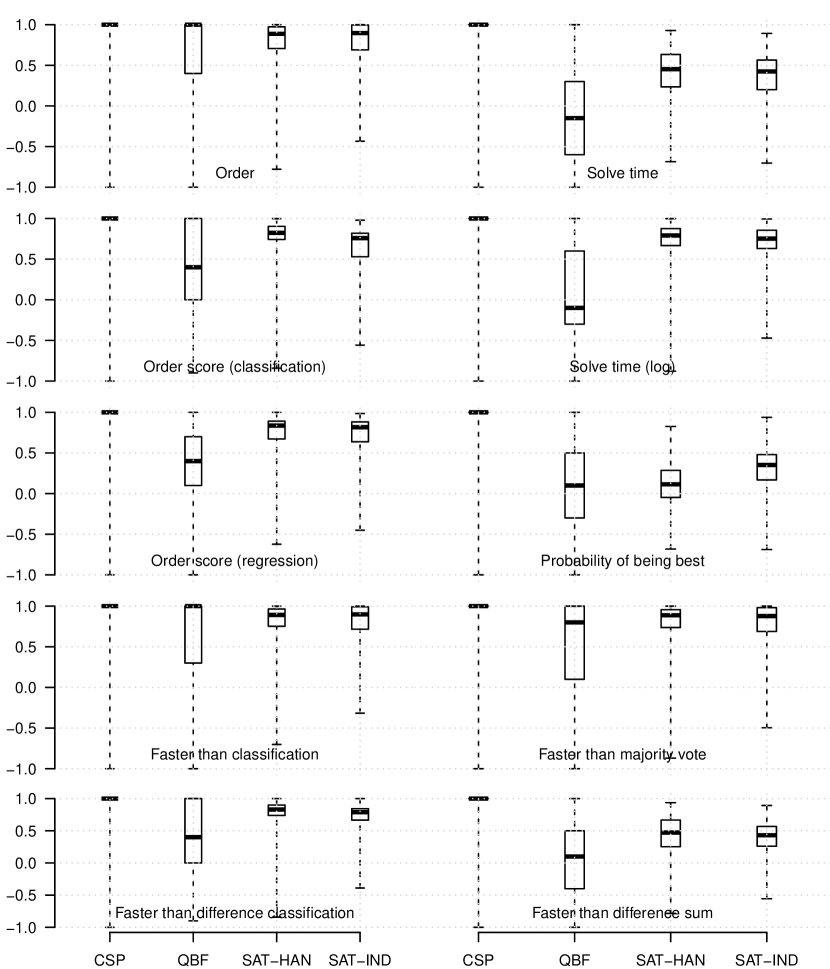
Figure 1: Results for the best machine learning algorithm for each data set and rank prediction approach. For each prediction approach, the best algorithm over all data sets is shown. The thick line in the center of the box corresponds to the median, the top and bottom ends of the box to the 75th and 25th percentile respectively and the top and bottom end of the whiskers to the maximum and minimum, respectively.

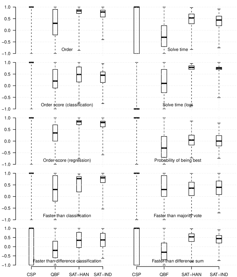
Figure 2: Results for the worst machine learning algorithm for each data set and rank prediction approach. For each prediction approach, the worst algorithm over all data sets is shown. The thick line in the center of the box corresponds to the median, the top and bottom ends of the box to the 75th and 25th percentile respectively and the top and bottom end of the whiskers to the maximum and minimum, respectively.

Figures 1 and 2 give the results for best and worst algorithms, respectively. The first observation is that for all rank prediction approaches and data sets, there is a large spread in the quality of the predicted rankings. However, most of the time the majority of predictions for the best algorithm is closer to 1 than 0, meaning that good rankings are achieved on average. In particular the median values are often very close to 1.

There are only two algorithms for the CSP data set and thus the ranking quality score will always be 1 or -1. The worse score occurs only in a few cases even for the worst machine learning algorithm and all approaches perform consistently well. Unfortunately this does not give us any information as to which approach is better. On the other data sets however, there is a larger number of algorithms and thus a much richer set of possible rankings. The results achieved on those data sets are more informative.

We are presenting the results for the both the best and the worst machine learning algorithm for each rank prediction approach. This way, we can provide a picture of the overall performance of each approach regardless of the underlying machine learning algorithm. All the approaches presented in this paper are agnostic to how the predictions they require are achieved.

In a real portfolio setting, the performance of the machine learning algorithm underlying any of our approaches would need to be tuned to get the best performance. In this paper, we do not do any tuning because our focus is not on the absolute performance, but on the performance differences between the approaches with everything else being equal.

The results shown in the figures are not immediately conclusive with respect to which rank prediction approaches provide the best performance. We present the results in aggregate form in tables 1 and 2.

	CSP	QBF	SAT-HAN	SAT-IND	total
Order	3	2.4	2.789	3.148	11.337
Order score (classification)	3	1.5	2.625	2.527	9.652
Order score (regression)	3	1.2	2.777	2.871	9.848
Faster than classification	3	2.3	2.907	3.29	11.497
Faster than difference classification	3	1.5	2.626	2.909	10.036
Solve time	3	-0.45	1.563	1.379	5.492
Solve time (log)	3	0.2	2.453	2.761	8.413
Probability of being best	3	0.3	0.496	1.25	5.046
Faster than majority vote	3	1.9	2.711	3.052	10.662
Faster than difference sum	3	0.2	1.544	1.594	6.338

Table 1: Sum of the ranking quality scores over all quartiles for all data sets and rank prediction approaches for the best machine learning algorithm for a particular prediction approach. Higher scores are better. All numbers are rounded to three decimal places.

	CSP	QBF	SAT-HAN	SAT-IND	total
Order	3	1	2.584	2.821	9.406
Order score (classification)	3	0.8	1.705	1.357	6.862
Order score (regression)	3	1.05	2.672	2.678	9.4
Faster than classification	3	1	1.981	2.741	8.722
Faster than difference classification	1	-0.5	1.246	1.454	3.2
Solve time	1	-0.8	1.667	1.409	3.275
Solve time (log)	-3	0.5	2.442	2.724	2.667
Probability of being best	3	-0.8	0.267	0.068	2.535
Faster than majority vote	3	1.2	1.226	1.44	6.866
Faster than difference sum	1	-0.8	1.667	1.409	3.275

Table 2: Sum of the ranking quality scores over all quartiles for all data sets and rank prediction approaches for the worst machine learning algorithm for a particular prediction approach. Higher scores are better. All numbers are rounded to three decimal places.

The tables show the sum of the quartiles of the Spearman correlation scores for all data sets and rank prediction approaches. Again we show the numbers for both the best and the worst machine learning algorithm. We decided to use the sum for comparison because it takes into account all the scores. In addition to the scores for the individual data sets, we show the total sum over all data sets.

The results demonstrate that some approaches are more susceptible than others to the performance of the underlying machine learning algorithms. This becomes clear from the spread between the best and worst algorithm – in some cases, there is almost no difference at all, whereas in other cases there is a significant difference.

The overall best approach is the Faster than classification approach, closely followed by the Order approach. The Faster than majority vote and Order score (regression) approaches exhibit good performance as well. Looking at the results for the worst machine learning algorithm, the best approach is Order, closely followed by Order score (regression), Faster than classification and Faster than majority vote.

The results shown in tables 1 and 2 are consistent with respect to which approaches perform well and which ones do not. In both cases, the worst approach is Probability of being best. This suggests that there is a difference between the different rank prediction approaches that is independent of the underlying machine learning algorithm.

We performed the Kruskal-Wallis rank sum test across the different approaches. The differences between the series of quartiles over all data sets were not statistically significant. The Wilcoxon signed-rank test for pairs of approaches did suggest statistically significant differences though. This suggests that there is not enough data to draw statistically significant conclusions on the entire set of approaches, but that there are differences.

The results clearly demonstrate that the relationship between the portfolio algorithms is important to take into account when predicting the ranking of algorithms. In general, the approaches that consider the algorithms only in isolation perform worse than the approaches that consider the portfolio as a whole or pairs of algorithms. The exception to this rule is the Order score (regression) approach, which consistently performs well.

While this result is intuitively plausible and not unexpected, this paper is the first to investigate it through rigorous empirical evaluation. While [23] use a similar approach that considers pairs of algorithms, they do not compare it to other approaches. We show conclusively that this is beneficial in terms of the similarity of the derived ranking to the actual ranking.

We were mildly surprised by the good performance of the Order approach. It is the conceptually simplest of the approaches we evaluated and the rationale for including it at all was only to provide a comparison to the other approaches. Nevertheless, it turns out that this simple approach is capable of producing good rankings even for portfolios with a relatively large number of solvers where the space of possible labels is large. This performance depends of course also on the number of rankings that are actually going to be predicted, as a potentially large subset of all rankings will never occur in the training data. With this caveat in mind, the Order approach can provide a reasonable starting point.

5.1 Performance in $\mathcal{R}$

Overall, the approaches in $\mathcal{R}_{1}$ perform better than those in $\mathcal{R}_{2}$. Out of five approaches at each level, only one in $\mathcal{R}_{2}$ features in the overall top four approaches. Level $\mathcal{R}_{2}$ also contains the overall worst approach. This is especially apparent in tables 1 and 2, where the top half of the table contains the approaches from $\mathcal{R}_{1}$ and the bottom half the ones from $\mathcal{R}_{2}$. In both tables, the top half is consistently better than the bottom half.

The reason for this is that the predictions approaches in $\mathcal{R}_{2}$ have to make are inherently more complex and there is more margin for error. Statistically, approaches that make simple predictions have a better chance of being correct simply by luck. While a machine learning approach would ideally be able to identify and exploit the relationship between problem features and the ranking of the portfolio algorithms, all statistical approaches such as the ones used here benefit from having a higher chance of being correct by pure luck.

It should be noted that the only criteria we use for evaluating the quality of an approach is the computed ranking itself. The approaches in $\mathcal{R}_{2}$ provide more information than that and, more importantly, are evaluated according to a different objective criteria during training. However, the two different objectives are closely linked. While our evaluation puts the approaches in $\mathcal{R}_{2}$ at a slight disadvantage, they still demonstrate good performance overall.

In the machine learning literature, great care is usually taken to train and evaluate according to the same objective criteria. We consciously do not restrict ourselves to the approaches in $\mathcal{R}_{1}$ to facilitate this, but include other approaches as well to give a better picture of the performance of a wider variety of methods. While this may seem strange to machine learning researchers, it is common practice in algorithm selection – the original SATzilla for example trained models to predict the performance of algorithms, but was evaluated in terms of how often the algorithm with the best predicted performance was the one with the actual best performance.

6 Conclusions and future work

We have presented and evaluated several approaches for predicting the ranking of algorithms from a portfolio on a particular problem. While there are a vast number of publications that propose and evaluate methods for choosing the best algorithm, few are concerned with predicting the complete ranking of the algorithms. This information is becoming increasingly relevant in many applications however, for example through the increase of the number of processors and thus the potential of running several algorithms at the same time.

Many approaches reported in the literature rely at least implicitly on rankings of algorithms, for example by computing schedules according to which to run the algorithms in a portfolio. Despite this, no study of how to make this prediction in practice has been presented so far. It is this gap in the literature that we have addressed in this paper.

In addition to the empirical evaluation of a range of approaches, we presented a framework to assess the power of predictions with respect to deriving a ranking. This allows us to classify the approaches that we have evaluated and compare their predictive output. Our framework was inspired by the theory of scales of measurement.

One of the main and most important conclusions of this paper is that rank prediction approaches that consider algorithms in isolation perform worse than approaches that consider them in combination. This is not surprising, given that a ranking is intrinsically concerned with the relationship of algorithms.

We identified the Faster than classification, Faster than majority vote and Order as the approaches that deliver the best overall performance. While some of these are complex and rely on layers of machine learning models, the Order approach is actually the simplest of those evaluated here. Its simplicity makes it easy to implement and an ideal starting point for researchers planning to predict rankings of algorithms. In addition to the approaches named above, predicting the order through a ranking score predicted by a regression algorithm achieved good performance.

In our proposed framework, most of the approaches that deliver good performance are in the level that provides simpler predictions. For many applications it is desirable however to have the additional information approaches at the higher level provides. Developing more approaches that are able to deliver this and provide good performance is a possible avenue for future work.

The question of how to predict a ranking of algorithms is only the first step for putting this approach to practical use. In the future, we would like to evaluate different practical approaches for using the rankings – for example running the top $n$ algorithms in parallel or computing an explicit schedule based on ranking scores. Using predicted rankings in practice poses additional challenges because not only the overall quality of the ranking matters, but also whether the algorithms with the best performance are actually at the top of the ranking.

Investigating this question is just one of the many possible avenues for future work. We believe that with the current explosion of the number of processors that are available even in consumer-grade machines and thus the increased ability to run more and more algorithms in parallel, the ability to reliably predict good rankings will be increasingly important for practical applications.

Acknowledgements

Lars Kotthoff is supported by European Union FP7 grant 284715.

References

- [1] Brazdil, P.B., Soares, C., Da Costa, J.P.: Ranking learning algorithms: Using IBL and meta-learning on accuracy and time results. Mach. Learn. 50(3), 251–277 (Mar 2003)
- [2] Gent, I.P., Jefferson, C., Kotthoff, L., Miguel, I., Moore, N., Nightingale, P., Petrie, K.: Learning when to use lazy learning in constraint solving. In: ECAI. pp. 873–878 (Aug 2010)
- [3] Gomes, C.P., Selman, B.: Algorithm portfolios. Artificial Intelligence 126(1-2), 43–62 (2001)
- [4] Hall, M., Frank, E., Holmes, G., Pfahringer, B., Reutemann, P., Witten, I.H.: The WEKA data mining software: An update. SIGKDD Explor. Newsl. 11(1), 10–18 (Nov 2009)
- [5] Howe, A.E., Dahlman, E., Hansen, C., Scheetz, M., von Mayrhauser, A.: Exploiting competitive planner performance. In: Proceedings of the Fifth European Conference on Planning. pp. 62–72. Springer (1999)
- [6] Huberman, B.A., Lukose, R.M., Hogg, T.: An economics approach to hard computational problems. Science 275(5296), 51–54 (1997)
- [7] Hurley, B., O’Sullivan, B.: Adaptation in a CBR-Based solver portfolio for the satisfiability problem. In: Case-Based Reasoning Research and Development. Lecture Notes in Computer Science, vol. 7466, pp. 152–166 (2012)
- [8] Kadioglu, S., Malitsky, Y., Sabharwal, A., Samulowitz, H., Sellmann, M.: Algorithm selection and scheduling. In: 17th International Conference on Principles and Practice of Constraint Programming. pp. 454–469 (2011)
- [9] Kanda, J., Soares, C., Hruschka, E., de Carvalho, A.: A meta-learning approach to select meta-heuristics for the traveling salesman problem using MLP-Based label ranking. In: 19th International Conference on Neural Information Processing. pp. 488–495. Springer-Verlag, Berlin, Heidelberg (2012)
- [10] Kotthoff, L.: Algorithm selection for combinatorial search problems: A survey. Tech. rep., University College Cork (2012)
- [11] Kotthoff, L.: Hybrid regression-classification models for algorithm selection. In: 20th European Conference on Artificial Intelligence. pp. 480–485 (Aug 2012)
- [12] Kotthoff, L., Gent, I.P., Miguel, I.: An evaluation of machine learning in algorithm selection for search problems. AI Communications 25(3), 257–270 (2012)
- [13] Leite, R., Brazdil, P.: Active testing strategy to predict the best classification algorithm via sampling and metalearning. In: ECAI. pp. 309–314 (2010)
- [14] O’Mahony, E., Hebrard, E., Holland, A., Nugent, C., O’Sullivan, B.: Using case-based reasoning in an algorithm portfolio for constraint solving. In: Proceedings of the 19th Irish Conference on Artificial Intelligence and Cognitive Science (Jan 2008)
- [15] Pulina, L., Tacchella, A.: A self-adaptive multi-engine solver for quantified boolean formulas. Constraints 14(1), 80–116 (2009)
- [16] Rice, J.R.: The algorithm selection problem. Advances in Computers 15, 65–118 (1976)
- [17] Roberts, M., Howe, A.E.: Directing a portfolio with learning. In: AAAI 2006 Workshop on Learning for Search (2006)
- [18] Soares, C., Brazdil, P.B., Kuba, P.: A meta-learning method to select the kernel width in support vector regression. Mach. Learn. 54(3), 195–209 (Mar 2004)
- [19] Stevens, S.S.: On the theory of scales of measurement. Science 103(2684), 677–680 (Jun 1946)
- [20] Streeter, M.J., Golovin, D., Smith, S.F.: Combining multiple heuristics online. In: Proceedings of the 22nd National Conference on Artificial Intelligence. vol. 2, pp. 1197–1203. AAAI Press (2007)
- [21] Vembu, S., Gärtner, T.: Label ranking algorithms: A survey. In: Fürnkranz, J., Hüllermeier, E. (eds.) Preference Learning, pp. 45–64. Springer Berlin Heidelberg (2011)
- [22] Xu, L., Hutter, F., Hoos, H.H., Leyton-Brown, K.: SATzilla: portfolio-based algorithm selection for SAT. J. Artif. Intell. Res. (JAIR) 32, 565–606 (2008)
- [23] Xu, L., Hutter, F., Hoos, H.H., Leyton-Brown, K.: Hydra-MIP: automated algorithm configuration and selection for mixed integer programming. In: Workshop on Experimental Evaluation of Algorithms for Solving Problems with Combinatorial Explosion. pp. 16–30 (2011)