Gravity as an emergent phenomenon:
experimental signatures

M. Consoli^a and A. Pluchino^a,b
a) Istituto Nazionale di Fisica Nucleare, Sezione di Catania
b) Dipartimento di Fisica e Astronomia dell’ Università di Catania

Abstract

According to some authors, gravity might be an emergent phenomenon in a fundamentally flat space-time. In this case the speed of light in the vacuum would not coincide exactly with the basic parameter $c$ entering Lorentz transformations and, for an apparatus placed on the Earth’s surface, light should exhibit a tiny fractional anisotropy at the level $10^{-15}$. We argue that, most probably, this effect is now observed in many room-temperature ether-drift experiments and, in particular, in a very precise cryogenic experiment where this level of signal is about 100 times larger than the designed short-term stability. To fully appreciate what is going on, however, one should consider the vacuum as a true physical medium whose fundamental quantum nature gives rise to the irregular, non-deterministic pattern which characterizes the observed signal.

1.  The usual interpretation of gravitational phenomena is in terms of a universal metric field $g_{\mu\nu}(x)$ viewed as a fundamental modification of flat space-time. Reconciling this interpretation with some basic aspects of the quantum theory may pose, however, some consistency problems, see e.g. [1] and references quoted therein. For this reason, one could try to explore a different approach where instead curvature is an emergent phenomenon [2, 3] in flat space-time analogously to the curvature of light in Euclidean space when propagating in a medium with variable density. This point of view may become natural if, by taking seriously the phenomenon of vacuum condensation in particle physics, the vacuum starts to be considered a true superfluid medium [4], i. e. a quantum liquid [5].

As a definite scenario, an effective metric tensor $g_{\mu\nu}(x)$ could then originate from local modifications of the basic space-time units and of the velocity of light which are known, see e.g. [6, 7, 8], to represent an alternative way to introduce the concept of curvature . The only possibly new aspect is that the scale over which $g_{\mu\nu}(x)$ varies (say a small fraction of millimeter or so) is taken much larger than any elementary particle, or nuclear, or atomic size [10]. In this sense, the type of description of classical general relativity, and of its possible variants, becomes similar to hydrodynamics that, concentrating on the properties of matter at scales larger than the mean free path for the elementary constituents, is insensitive to the details of the underlying molecular dynamics.

By following this interpretation, one could first consider the simplest two-parameter scheme of an effective isotropic metric

$${g}_{\mu\nu}={\rm diag}(A,-B,-B,-B)$$ (1)

This depends on two functions which, in a flat-space picture, can be interpreted in terms of an overall re-scaling $\lambda$ of the space-time units and of a refractive index ${\cal N}$ so that $A=c^{2}{{\lambda^{2}}\over{{\cal{N}}^{2}}}$ and $B=\lambda^{2}$. Now, since physical units of time scale as inverse frequencies, and the measured frequencies $\hat{\omega}$ for a Newtonian potential $U_{N}\neq 0$ are red-shifted when compared to the corresponding value $\omega$ for $U_{N}=0$, this fixes the value of $\lambda$. Furthermore, independently of any specific underlying mechanism, the two functions $A$ and $B$ can be related through the general requirement $AB=c^{2}=$ constant which expresses the basic property of light of being, at the same time, a corpuscular and undulatory phenomenon [10]. This fixes the value of ${\cal N}$ giving the structure

$${\cal{N}}\sim 1+2{{|U_{N}|}\over{c^{2}}}~{}~{}~{}~{}~{}~{}~{}~{}~{}~{}~{}~{}~{}~{}~{}~{}~{}~{}~{}~{}~{}~{}~{}~{}~{}~{}\lambda\sim 1+{{|U_{N}|}\over{c^{2}}}$$ (2)

which to first order is equivalent to general relativity. Finally more complicated metrics with off-diagonal elements $g_{0i}\neq 0$ and $g_{ij}\neq 0$ can be obtained by applying boosts and rotations to Eq.(1). This basically reproduces the picture of the curvature effects in a moving fluid with a metric tensor which depends on $\varphi={{U_{N}}\over{c^{2}}}$ in a definite parametric form, i.e. $g_{\mu\nu}(x)=g_{\mu\nu}[\varphi(x)]$. In this way, a first consistency check of an emergent-gravity approach consists in constructing some long-wavelength vacuum excitation $\varphi(x)$ that, on a coarse grained scale, behaves as the Newtonian potential [10] .

Being faced with two alternative interpretations, one may wonder whether the basic conceptual difference with standard general relativity could have phenomenological implications . Our scope here is to refine and update the analysis of [11] namely : i) in principle, one expects a non-zero fractional anisotropy ${\cal O}(10^{-15})$ of the velocity of light in the vacuum ii) if the vacuum is considered a quantum medium there are non-trivial implications for the analysis of the experiments iii) most probably, this tiny effect is now observed in many room-temperature ether-drift experiments and, in particular, in a very precise cryogenic experiment [12] where the level ${\cal O}(10^{-15})$ is now about 100 times larger than the designed short-term stability.

2.  For the problem of measuring the speed of light, we shall follow closely ref.[11] (to which we address the reader for more details). The main point is that, to determine speed as (distance moved)/(time taken), one must first choose some standards of distance and time. Since different choices can give different answers, we shall adopt the point of view of special relativity: the right space-time units are those for which the speed of light in the vacuum $c_{\gamma}$, when measured in an inertial frame, coincides with the basic parameter $c$ entering Lorentz transformations. However, inertial frames are just an idealization. Therefore the appropriate realization is to assume local standards of distance and time such that the identification $c_{\gamma}=c$ holds as an asymptotic relation in the physical conditions which are as close as possible to an inertial frame, i.e. in a freely falling frame (at least by restricting to a space-time region small enough that tidal effects of the external gravitational potential $U_{\rm ext}(x)$ can be ignored). This is essential to obtain an operative definition of the otherwise unknown parameter $c$.

With these premises, light propagation for an observer $S^{\prime}$ sitting on the Earth’s surface can be described with increasing degrees of approximations:

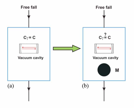
Figure 1: A pictorial representation of the effect of a heavy mass $M$ carried on board of a freely-falling system, case (b). With respect to case (a), in a flat-space picture of gravity, the mass $M$ modifies the effective, local space-time structure by re-scaling the physical units ($dx$, $dy$, $dz$, $dt$) $\to$ ($d\hat{x}$, $d\hat{y}$, $d\hat{z}$, $d\hat{t}$) and introducing a non-trivial refractive index ${\cal N}\neq 1$ so that now $c_{\gamma}\neq c$. The figure is taken from ref.[13].

i) $S^{\prime}$ is considered a freely falling frame. This amounts to assume $c_{\gamma}=c$ so that, given two events which, in terms of the local space-time units of $S^{\prime}$, differ by $(dx,dy,dz,dt)$, light propagation is described by the condition (ff=’free-fall’)

$$(ds^{2})_{\rm ff}=c^{2}dt^{2}-(dx^{2}+dy^{2}+dz^{2})=0~{}$$ (3)

ii) To a closer look, however, an observer $S^{\prime}$ placed on the Earth’s surface can only be considered a freely-falling frame up to the presence of the Earth’s gravitational field. Its inclusion can be estimated by considering $S^{\prime}$ as a freely-falling frame, in the same external gravitational field described by $U_{\rm ext}(x)$, that however is also carrying on board a heavy object of mass $M$ (the Earth’s mass itself) that affects the effective local space-time structure, see Fig.1. To derive the required correction, let us again denote by ($dx$, $dy$, $dz$, $dt$) the local space-time units of the freely-falling observer $S^{\prime}$ in the limit $M=0$ and by $\delta U$ the extra Newtonian potential produced by the heavy mass $M$ at the experimental set up where one wants to describe light propagation. From Eqs.(1) and (2), light propagation for the $S^{\prime}$ observer is now described by re-scaled units ($d\hat{x}$, $d\hat{y}$, $d\hat{z}$, $d\hat{t}$) and a refractive index as

$$(ds^{2})_{\rm\delta U}={{c^{2}d\hat{t}^{2}}\over{{\cal N}^{2}}}-(d\hat{x}^{2}+d\hat{y}^{2}+d\hat{z}^{2})=0~{}$$ (4)

where, to first order in $\delta U$, the re-scaling $\lambda$ and ${\cal N}$ are

$$\lambda\sim 1+{{|\delta U|}\over{c^{2}}}~{}~{}~{}~{}~{}~{}~{}~{}~{}~{}~{}~{}~{}~{}~{}~{}~{}~{}~{}~{}~{}~{}~{}~{}{\cal N}\sim 1+2{{|\delta U|}\over{c^{2}}}$$ (5)

As anticipated, to this order, the metric is formally as in general relativity

$$(ds^{2})_{\rm GR}=c^{2}dT^{2}(1-2{{|U_{\rm N}|}\over{c^{2}}})-(dX^{2}+dY^{2}+dZ^{2})(1+2{{|U_{\rm N}|}\over{c^{2}}})\equiv c^{2}d\tau^{2}-dl^{2}$$ (6)

where $U_{N}$ denotes the Newtonian potential and ($dT$, $dX$, $dY$, $dZ$) arbitrary coordinates defined for $U_{\rm N}=0$. Finally, $d\tau$ and $dl$ denote the elements of proper time and proper length in terms of which, in general relativity, one would again deduce from $ds^{2}=0$ the same universal value $c={{dl}\over{d\tau}}$. This is the basic difference with Eqs.(4), (5) where the physical unit of length is $\sqrt{d\hat{x}^{2}+d\hat{y}^{2}+d\hat{z}^{2}}$, the physical unit of time is $d\hat{t}$ and instead a non-trivial refractive index ${\cal N}$ is introduced. For an observer placed on the Earth’s surface, its value is

$${\cal N}-1\sim{{2G_{N}M}\over{c^{2}R}}\sim 1.4\cdot 10^{-9}$$ (7)

$M$ and $R$ being respectively the Earth’s mass and radius.

iii) Differently from general relativity, in a flat-space interpretation with re-scaled units ($d\hat{x}$, $d\hat{y}$, $d\hat{z}$, $d\hat{t}$) and ${\cal N}\neq 1$, the speed of light in the vacuum $c_{\gamma}$ no longer coincides with the parameter $c$ entering Lorentz transformations. Therefore, as a general consequence of Lorentz transformations, an isotropic propagation as in Eq.(4) can only be valid for a special state of motion of the Earth’s laboratory. This provides the operative definition of a preferred reference frame $\Sigma$ while for a non-zero relative velocity ${\bf V}$ there are off diagonal elements $g_{0i}\neq 0$ in the effective metric and a tiny light anisotropy. These off diagonal elements can be imagined as being due to a directional polarization of the vacuum induced by the now moving Earth’s gravitational field and express the general property [14] that any metric, locally, can always be brought into diagonal form by suitable rotations and boosts. As shown in ref.[11], to first order in both $({\cal N}-1)$ and $V/c$ one finds

$$g_{0i}\sim 2({\cal N}-1){{V_{i}}\over{c}}$$ (8)

In this way, by introducing $\beta=V/c$, $\kappa=({\cal N}^{2}-1)$ and the angle $\theta$ between ${\bf V}$ and the direction of light propagation, one finds, to ${\cal O}(\kappa)$ and ${\cal O}(\beta^{2})$, the one-way velocity [11]

$$c_{\gamma}(\theta)={{c}\over{{\cal N}}}~{}\left[1-\kappa\beta\cos\theta-{{\kappa}\over{2}}\beta^{2}(1+\cos^{2}\theta)\right]$$ (9)

and a two-way velocity

$$\bar{c}_{\gamma}(\theta) = {{2c_{\gamma}(\theta)c_{\gamma}(\pi+\theta)}\over{c_{\gamma}(\theta)+c_{\gamma}(\pi+\theta)}}$$ (10)

$$\sim {{c}\over{{\cal N}}}~{}\left[1-\kappa\beta^{2}\left(1-{{1}\over{2}}\sin^{2}\theta\right)\right]$$

This gives finally

$${{\bar{c}_{\gamma}(\pi/2+\theta)-\bar{c}_{\gamma}(\theta)}\over{\langle\bar{c}_{\gamma}\rangle}}\sim({\cal N}-1){{v^{2}}\over{c^{2}}}\cos 2(\theta-\theta_{0})$$ (11)

where the pair $(v,\theta_{0})$ describes the projection of ${\bf{V}}$ onto the relevant plane. From the previous analysis, by using Eq.(7) and adopting, as a rough order of magnitude, the typical value of most cosmic motions $V\sim$ 300 km/s, one thus expects a tiny fractional anisotropy

$${{\langle\Delta\bar{c}_{\theta}\rangle}\over{c}}\sim({\cal N}-1){{V^{2}}\over{c^{2}}}={\cal O}(10^{-15})$$ (12)

that could finally be detected in the present, precise ether-drift experiments.

3. In present ether-drift experiments one measures the frequency shift, i.e. the beat signal, $\Delta\nu$ of two rotating optical resonators whose definite non-zero value would provide a direct measure of an anisotropy of the velocity of light [16]. In this framework, the possible time modulation of the signal that might be induced by the Earth’s rotation (and its orbital revolution) has always represented a crucial ingredient for the analysis of the data. To see this, let us re-write Eq.(11) as

$${{\Delta\nu(t)}\over{\nu_{0}}}={{\Delta\bar{c}_{\theta}(t)}\over{c}}\sim({\cal N}-1){{v^{2}(t)}\over{c^{2}}}\cos 2(\omega_{\rm rot}t-\theta_{0}(t))$$ (13)

where $\nu_{0}$ indicates the reference frequency of the two resonators and $\omega_{\rm rot}$ is the rotation frequency of the apparatus. Therefore one finds

$${{\Delta\nu(t)}\over{\nu_{0}}}\sim 2{S}(t)\sin 2\omega_{\rm rot}t+2{C}(t)\cos 2\omega_{\rm rot}t$$ (14)

with

$$C(t)={{1}\over{2}}({\cal N}-1)~{}{{v^{2}_{x}(t)-v^{2}_{y}(t)}\over{c^{2}}}~{}~{}~{}~{}~{}~{}~{}~{}~{}~{}~{}~{}~{}~{}~{}~{}~{}~{}~{}~{}S(t)={{1}\over{2}}({\cal N}-1)~{}{{2v_{x}(t)v_{y}(t)}\over{c^{2}}}$$ (15)

and $v_{x}(t)=v(t)\cos\theta_{0}(t)$, $v_{y}(t)=v(t)\sin\theta_{0}(t)$

The standard assumption to analyze the data is to consider a cosmic Earth’s velocity with well defined magnitude $V$, right ascension $\alpha$ and angular declination $\gamma$ that can be considered constant for short-time observations of a few days where there are no appreciable changes due to the Earth’s orbital velocity around the Sun. In this framework, where the only time dependence is due to the Earth’s rotation, one identifies $v(t)\equiv\tilde{v}(t)$ and $\theta_{0}(t)\equiv\tilde{\theta}_{0}(t)$ where $\tilde{v}(t)$ and $\tilde{\theta}_{0}(t)$ derive from the simple application of spherical trigonometry [11]

$$\cos z(t)=\sin\gamma\sin\phi+\cos\gamma\cos\phi\cos(\tau-\alpha)$$ (16)

$$\tilde{v}(t)=V\sin z(t)$$ (17)

$$\tilde{v}(t)\cos\tilde{\theta}_{0}(t)=V\left[\sin\gamma\cos\phi-\cos\gamma\sin\phi\cos(\tau-\alpha)\right]$$ (18)

$$\tilde{v}(t)\sin\tilde{\theta}_{0}(t)=V\cos\gamma\sin(\tau-\alpha)$$ (19)

Here $z=z(t)$ is the zenithal distance of ${\bf{V}}$, $\phi$ is the latitude of the laboratory, $\tau=\omega_{\rm sid}t$ is the sidereal time of the observation in degrees ($\omega_{\rm sid}\sim{{2\pi}\over{23^{h}56^{\prime}}}$) and the angle $\theta_{0}$ is counted conventionally from North through East so that North is $\theta_{0}=0$ and East is $\theta_{0}=90^{o}$. In this way, one finds

$$S(t)\equiv{\tilde{S}}(t)={S}_{s1}\sin\tau+{S}_{c1}\cos\tau+{S}_{s2}\sin(2\tau)+{S}_{c2}\cos(2\tau)$$ (20)

$$C(t)\equiv{\tilde{C}}(t)={C}_{0}+{C}_{s1}\sin\tau+{C}_{c1}\cos\tau+{C}_{s2}\sin(2\tau)+{C}_{c2}\cos(2\tau)$$ (21)

In this picture, the $C_{k}$ and $S_{k}$ Fourier coefficients depend on the three parameters $(V,\alpha,\gamma)$ (see [16]) and, to very good approximation, should be time-independent for short-time observations. Thus, by accepting this theoretical framework, it becomes natural to average the various $C_{k}$ and $S_{k}$ obtained from fits performed during a 1$-$2 day observation period. In this case, although the typical instantaneous $S(t)$ and $C(t)$ are ${\cal O}(10^{-15})$, due to the irregular nature of the observed signal, there are strong cancelations with global averages $(C_{k})^{\rm avg}$ and $(S_{k})^{\rm avg}$ for the Fourier coefficients at the level ${\cal O}(10^{-17})$ [17, 18]. This is usually taken as an indication that the much larger instantaneous signal is a spurious instrumental effect, e.g. thermal noise.

However, there might be forms of ether-drift where the straightforward parameterizations Eqs.(20), (21) and the associated averaging procedures are not allowed. For this reason, before assuming any definite theoretical scenario, one could first ask: if light were really propagating in a physical medium, an ether, and not in a trivial empty vacuum, how should the motion of (or in) this medium be described? Namely, could this relative motion exhibit variations that are not only due to known effects as the Earth’s rotation and orbital revolution? Here, there is the logical gap. In fact, by comparing the Earth’s cosmic motion with that of a body in a fluid, the standard picture Eqs.(16)$-$(21) amounts to the condition of a pure laminar flow where global and local velocity fields coincide. Instead, the relation between the macroscopic Earth’s motion and the measurements performed in a laboratory depends on the physical nature of the vacuum. If we consider the vacuum as a superfluid, i.e. a quantum liquid, then the frequency shifts will likely exhibit the typical irregular, non-deterministic pattern which characterizes any quantum measurement. In this case, in view of the striking similarities [19] between many aspects of turbulence in fluids and superfluids, and of the intriguing derivation of Kolmogorov scaling laws [20] from quantum hydrodynamics [21], rather than adopting the simple classical model of a laminar flow, one could try to compare the experimental data with models of a turbulent flow, see Fig.2. In this alternative scenario, the same basic experimental data might admit a different interpretation and a genuine stochastic signal $\Delta\nu(t)\neq 0$ could perfectly coexist with $(C_{k})^{\rm avg}\sim(S_{k})^{\rm avg}\sim 0$.

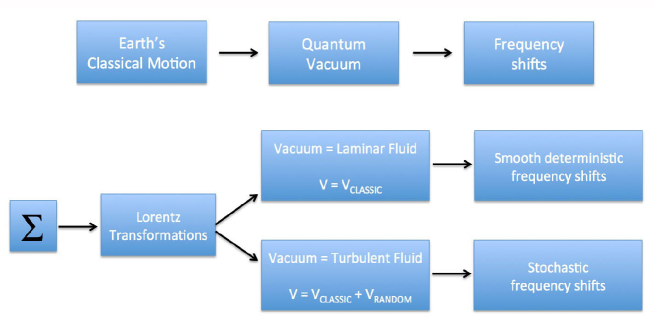
Figure 2: The two possible ways to relate Earth’s classical motion and frequency shifts.

4. By considering the vacuum as a fluid, one is naturally driven to the limit of zero viscosity where the local velocity field becomes non-differentiable and the ordinary formulation in terms of differential equations becomes inadequate [22]. Thus, one has to adopt some other description, for instance a formulation in terms of random Fourier series [22, 23]. In this other approach, the parameters of the macroscopic motion are only used to fix the limiting boundaries [24] for a microscopic velocity field which has instead an intrinsic stochastic nature.

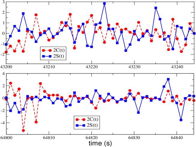
Figure 3: Two typical sets of 45 seconds for the instantaneous $2C(t)$ and $2S(t)$ in units $10^{-15}$. The two sets belong to the same random sequence and refer to two sidereal times that differ by 6 hours. The boundaries of the stochastic velocity components in Eqs.(22) and (23) are controlled by $(V,\alpha,\gamma)_{\rm CMB}$ through Eqs.(17) and (25).

The simplest choice, adopted in ref.[25], corresponds to a turbulence which, at small scales, appears statistically homogeneous and isotropic . This represents a zeroth-order approximation but, nevertheless, it is useful to illustrate basic phenomenological features associated with an underlying stochastic vacuum. The perspective is that of an observer moving in the turbulent fluid who wants to simulate the two components of the velocity in his x-y plane, at a given fixed location in his laboratory, to reproduce the $S(t)$ and $C(t)$ functions Eq.(15). In a statistically homogeneous turbulence, one finds the general expressions

$$v_{x}(t)=\sum^{\infty}_{n=1}\left[x_{n}(1)\cos\omega_{n}t+x_{n}(2)\sin\omega_{n}t\right]$$ (22)

$$v_{y}(t)=\sum^{\infty}_{n=1}\left[y_{n}(1)\cos\omega_{n}t+y_{n}(2)\sin\omega_{n}t\right]$$ (23)

where $\omega_{n}=2n\pi/T$, T being a time scale which represents a common period of all stochastic components. For numerical simulations, the typical value $T=T_{\rm day}$= 24 hours was adopted [25]. However, it was also checked with a few runs that the statistical distributions of the various quantities do not change substantially by varying $T$ in the rather wide range $0.1~{}T_{\rm day}\leq T\leq 10~{}T_{\rm day}$.

The coefficients $x_{n}(i=1,2)$ and $y_{n}(i=1,2)$ are random variables with zero mean and have the physical dimension of a velocity. Without necessarily assuming statistical isotropy, let us denote by $[-\tilde{v}_{x}(t),\tilde{v}_{x}(t)]$ the range for $x_{n}(i=1,2)$ and by $[-\tilde{v}_{y}(t),\tilde{v}_{y}(t)]$ the corresponding range for $y_{n}(i=1,2)$. In terms of these boundaries, the only non-vanishing (quadratic) statistical averages are

$$\langle x^{2}_{n}(i=1,2)\rangle_{\rm stat}={{{\tilde{v}}^{2}_{x}(t)}\over{3~{}n^{2\eta}}}~{}~{}~{}~{}~{}~{}~{}~{}~{}~{}~{}~{}~{}~{}~{}~{}~{}~{}~{}~{}~{}~{}~{}~{}~{}~{}~{}~{}\langle y^{2}_{n}(i=1,2)\rangle_{\rm stat}={{{\tilde{v}}^{2}_{y}(t)}\over{3~{}n^{2\eta}}}$$ (24)

in a uniform probability model within the intervals $[-\tilde{v}_{x}(t),\tilde{v}_{x}(t)]$ and $[-\tilde{v}_{y}(t),\tilde{v}_{y}(t)]$. Here, the exponent $\eta$ controls the power spectrum of the fluctuating components. For numerical simulations, between the two values $\eta=5/6$ and $\eta=1$ reported in ref.[24], we have adopted $\eta=1$ which corresponds to the point of view of an observer moving in the fluid.

As definite boundaries one could choose for instance $\tilde{v}_{x}(t)\equiv\tilde{v}(t)\cos\tilde{\theta}_{0}(t)$, $\tilde{v}_{y}(t)\equiv\tilde{v}(t)\sin\tilde{\theta}_{0}(t)$, $\tilde{v}(t)$ and $\tilde{\theta}_{0}(t)$ being defined in Eqs. (16)$-$(17). In this case, the set $V=$ 370 km/s, $\alpha=168$ degrees, $\gamma=-6$ degrees, which describes the average Earth’s motion with respect to the CMB, was shown [26] to provide a good statistical description of Joos’1930 observations [27] whose fringe-shift amplitudes $A(t)$, differently from the phases $\theta_{0}(t)$, can be extracted unambiguously from the original article. Finally, while still preserving $\tilde{v}^{2}_{x}(t)+\tilde{v}^{2}_{y}(t)=\tilde{v}^{2}(t)$, one could enforce statistical isotropy, in agreement with Kolmogorov’s theory, by choosing the common value from Eq.(17)

$$\tilde{v}_{x}(t)=\tilde{v}_{y}(t)={{\tilde{v}(t)}\over{\sqrt{2}}}$$ (25)

For such isotropic model, by combining Eqs.(22)$-$(25) one gets

$$\langle v^{2}_{x}(t)\rangle_{\rm stat}=\langle v^{2}_{y}(t)\rangle_{\rm stat}={{\tilde{v}^{2}(t)}\over{2}}~{}{{1}\over{3}}\sum^{\infty}_{n=1}{{1}\over{n^{2}}}~{}~{}~{}~{}~{}~{}~{}~{}~{}~{}~{}~{}~{}~{}~{}~{}~{}~{}~{}~{}~{}~{}~{}~{}\langle v_{x}(t)v_{y}(t)\rangle_{\rm stat}=0$$ (26)

with vanishing statistical averages $\langle C(t)\rangle_{\rm stat}=0$ and $\langle S(t)\rangle_{\rm stat}=0$ at any time $t$.

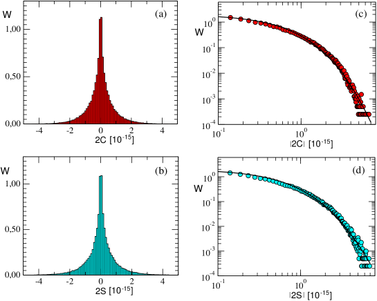
Figure 4: We show, see (a) and (b), the histograms $W$ obtained from a single simulation of measurements of $\rm 2C=2C(t)$ and $\rm 2S=2S(t)$ performed at regular steps of 1 second over an entire sidereal day . The vertical normalization is to a unit area. The mean values are $\rm\langle 2C\rangle_{\rm day}=-1.6\cdot 10^{-18}$, $\rm\langle 2S\rangle_{\rm day}=4.3\cdot 10^{-18}$ and the standard deviations $\rm\sigma_{\rm day}(2C)=0.87\cdot 10^{-15}$, $\rm\sigma_{\rm day}(2S)=0.96\cdot 10^{-15}$. We also show, see (c) and (d), the corresponding plots in a log-log scale and the fits with Eq.(27). The boundaries of the stochastic velocity components in Eqs.(22) and (23) are controlled by $(V,\alpha,\gamma)_{\rm CMB}$ through Eqs.(17) and (25).

To have an idea of the signal in this case, we report in Fig.3 two typical sets of the instantaneous values for $2C(t)$ and $2S(t)$ during one rotation period $T_{\rm rot}=$ 45 seconds of the apparatus of ref.[17]. The two sets belong to the same random sequence and refer to two sidereal times that differ by 6 hours. As in [26], the set $(V,\alpha,\gamma)_{\rm CMB}$ was adopted to control the boundaries of the stochastic velocity components through Eqs.(17)and (25). The value $\phi=52$ degrees was also fixed to reproduce the average latitude of the laboratories in Berlin and Düsseldorf.

We have also simulated long sequences of measurements performed at regular steps of 1 second over an entire sidereal day. For a particular random sequence, the resulting histograms of $2C$ and $2S$ are reported in panels (a) and (b) of Fig.4. Notice that these distributions are clearly “fat-tailed” and very different from a Gaussian shape. This kind of behavior is characteristic of probability distributions for instantaneous data in turbulent flows (see e.g. [28, 29]). To better appreciate the deviation from Gaussian behavior, in panels (c) and (d) we plot the same data in a log$-$log scale. The resulting distributions are well fitted by the so-called $q-$exponential function [30]

$$f_{q}(x)=a(1-(1-q)xb)^{1/(1-q)}$$ (27)

with entropic index $q\sim 1.1$. In view of Eqs.(26) any non-zero average $\langle 2C\rangle_{\rm day}$ and $\langle 2S\rangle_{\rm day}$ should be considered as statistical fluctuation. On the other hand, the standard deviations $\sigma(2C)$ and $\sigma(2S)$ have definite non-zero values

$$\sigma_{\rm day}(2C)\sim(0.87\pm 0.08)\cdot 10^{-15}~{}~{}~{}~{}~{}~{}~{}~{}~{}~{}~{}~{}~{}~{}~{}~{}~{}~{}\sigma_{\rm day}(2S)\sim(0.96\pm 0.09)\cdot 10^{-15}$$ (28)

where uncertainties reflect the observed variations due to the truncation of the Fourier modes in Eqs.(22), (23) and to the dependence on the random sequence.

Another reliable indicator is the statistical average of the amplitude of the signal $A(t)\equiv 2\sqrt{S^{2}(t)+C^{2}(t)}$. In this case, by using Eqs. (7) and (26), one finds

$$\langle A(t)\rangle_{\rm stat}=({\cal N}-1){{\tilde{v}^{2}(t)}\over{c^{2}}}~{}{{1}\over{3}}\sum^{\infty}_{n=1}{{1}\over{n^{2}}}={{\pi^{2}}\over{18}}~{}1.4\cdot 10^{-15}{{\tilde{v}^{2}(t)}\over{(300~{}{\rm km/s})^{2}}}$$ (29)

By maintaining the CMB parameters $(V,\alpha,\gamma)_{\rm CMB}$ and fixing $\phi=52$ degrees, one gets a daily average $\sqrt{\langle\tilde{v}^{2}\rangle}_{\rm day}\sim 332$ km/s from the relation [11]

$$\langle\tilde{v}^{2}\rangle_{\rm day}=V^{2}\left(1-\sin^{2}\gamma\sin^{2}\phi-{{1}\over{2}}\cos^{2}\gamma\cos^{2}\phi\right)$$ (30)

In this way, one predicts an average amplitude $\langle A\rangle_{\rm day}\sim 10^{-15}$. Notice however that, by performing extensive simulations, there are occasionally large spikes of the instantaneous amplitude, up to $(6\div 7)\cdot 10^{-15}$, when many Fourier modes sum up coherently (see the tails in panels (c) and (d) of Fig.4). The effect of these spikes gets smoothed when averaging but their presence is characteristic of a stochastic model. With a standard attitude, where one only expects smooth time modulations, the observation of such spikes would naturally be interpreted as a spurious disturbance. More precise tests of the model could be performed if real data for $A(t)$, $S(t)$ and $C(t)$ will become available.

5. An instantaneous stochastic signal $\sim 10^{-15}$ is well consistent with the most precise room temperature experiments [17, 18]. Since this observed value is comparable to the theoretical estimate of ref.[31], this has been interpreted in terms of thermal noise in the mirrors and the spacers of the optical resonators. However, as pointed out in ref.[11], this interpretation is not unique because roughly the same value is also obtained from cryogenic experiments [32, 33, 12]. The point is that the standard estimate of thermal disturbances [31] is based on the fluctuation-dissipation theorem, and therefore there is no obvious reason why room temperature and cryogenic resonators should exhibit the same instrumental effects. The unexplained agreement with the very recent result of ref.[12] is particularly striking in view of the factor 100 which now exists between observed stochastic signal $10^{-15}$ and designed short-term stability ${\cal O}(10^{-17})$. Tentatively, the authors of [12] interpret this discrepancy in terms of a lack of rigidity of their cryostat. However, probably, they have not considered the possibility of a genuine random signal and of intrinsic limitations placed by the vacuum structure. In this different perspective, the interpretation proposed here should also be taken into account for its ultimate implications.

References

- [1] S. Sonego, Phys. Lett. A208 (1995) 1.
- [2] C. Barcelo, S. Liberati and M. Visser, Class. Quantum Grav. 18 (2001) 3595.
- [3] M. Visser, C. Barcelo and S. Liberati, Gen. Rel. Grav. 34 (2002) 1719.
- [4] G. E. Volovik, Phys. Rep. 351 (2001) 195.
- [5] M. Consoli, Phys. Lett. A 376 (2012) 3377.
- [6] R. P. Feynman, R. B. Leighton and M. Sands, The Feynman Lectures on Physics, Addison Wesley Publ. Co. 1963, Vol.II, Chapt. 42.
- [7] R. H. Dicke, Phys. Rev. 125(1962) 2163 .
- [8] R. D’E. Atkinson, Proc. R. Soc. 272(1963) 60 .
- [9] K. Thorne, Black Holes and Time Warps: Einstein’s Outrageous Legacy, W. W. Norton and Co. Inc, New York and London, 1994, see Chapt. 11 ’What is Reality?’.
- [10] M. Consoli, Class. Quantum Grav. 26 (2009) 225008.
- [11] M. Consoli and L. Pappalardo, Gen. Rel. and Grav. 42 (2010) 2585.
- [12] M. Nagel et al., Ultra-stable Cryogenic Optical Resonators For Tests Of Fundamental Physics, arXiv:1308.5582[physics.optics].
- [13] M. Consoli, A. Pluchino and A. Rapisarda, Chaos, Solitons and Fractals 44(2011) 1089.
- [14] A. M. Volkov, A. A. Izmest’ev and G. V. Skrotskij, Sov. Phys. JETP 32, 686 (1971).
- [15] M. Consoli and E. Costanzo, Phys. Lett. A333 (2004) 355.
- [16] For a comprehensive review, see H. Müller et al., Appl. Phys. B 77 (2003) 719.
- [17] S. Herrmann, et al., Phys.Rev. D 80(2009) 105011.
- [18] Ch. Eisele, A. Newsky and S. Schiller, Phys. Rev. Lett. 103(2009) 090401 .
- [19] W. F. Vinen, Phys. Rev. B 61 (2000) 1410.
- [20] A. N. Kolmogorov, Dokl. Akad. Nauk SSSR 30 (1940) 4.
- [21] D. Drosdoff et al., arXiv:0903.0105[cond-matter.other].
- [22] L. Onsager, Nuovo Cimento, Suppl. 6 (1949) 279.
- [23] L. D. Landau and E. M. Lifshitz, Fluid Mechanics, Pergamon Press 1959, Chapt. III.
- [24] J. C. H. Fung et al., J. Fluid Mech. 236 (1992) 281.
- [25] M. Consoli, A. Pluchino, A. Rapisarda and S. Tudisco, Physica A394 (2013) 61.
- [26] M. Consoli, C. Matheson and A. Pluchino, Eur. Phys. J. Plus 128 (2013) 71.
- [27] G. Joos, Ann. d. Physik 7 (1930) 385.
- [28] K. R. Sreenivasan, Rev. Mod. Phys. 71, Centenary Volume 1999, S383.
- [29] C. Beck, Phys. Rev. Lett. 98, 064502 (2007).
- [30] C. Tsallis, Introduction to Nonextensive Statistical Mechanics, Springer, 2009.
- [31] K. Numata, A, Kemery and J. Camp, Phys. Rev. Lett. 93, 250602 (2004).
- [32] H. Müller, et al. Phys. Rev. Lett. 91 (2003) 020401 .
- [33] P. Antonini, M. Okhapkin, S. Göklu and S. Schiller, Phys. Rev. A71 (2005) 050101(R).