A MALT90 study of the chemical properties of massive clumps and filaments of infrared dark clouds

Abstract

Context. Infrared dark clouds (IRDCs) provide a useful testbed in which to investigate the genuine initial conditions and early stages of massive-star formation.

Aims. We attempt to characterise the chemical properties of a sample of 35 massive clumps of IRDCs through multi-molecular line observations. We also search for possible evolutionary trends among the derived chemical parameters.

Methods. The clumps are studied using the MALT90 line survey data obtained with the Mopra 22-m telescope. The survey covers 16 different transitions near 90 GHz. The spectral-line data are used in concert with our previous APEX/LABOCA 870-$\mu$m dust emission data.

Results. Eleven MALT90 transitions are detected towards the clumps at least at the $3\sigma$ level. Most of the detected species (SiO, C₂H, HNCO, HCN, HCO⁺, HNC, HC₃N, and N₂H⁺) show spatially extended emission towards many of the sources. The fractional abundances of the molecules with respect to H₂ are mostly found to be comparable to those determined in other recent similar studies of IRDC clumps (Vasyunina et al. 2011, A&A, 527, A88; Sanhueza et al. 2012, ApJ, 756, 60). We found that the abundances of SiO, HNCO, and HCO⁺ are higher in IR-bright clumps than in IR-dark sources, reflecting a possible evolutionary trend. A hint of such a trend is also seen for HNC and HC₃N. An opposite trend is seen for the C₂H and N₂H⁺ abundances. Moreover, a positive correlation is found between the abundances of HCO⁺ and HNC, and between those of HNC and HCN. The HCN and HNC abundances also appear to increase as a function of the N₂H⁺ abundance. The HNC/HCN and N₂H⁺/HNC abundance ratios are derived to be near unity on average, while that of HC₃N/HCN is $\sim 10\%$. The N₂H⁺/HNC ratio appears to increase as the clump evolves, while the HNC/HCO⁺ ratio shows the opposite behaviour.

Conclusions. The detected SiO emission is likely caused by shocks driven by outflows in most cases, although shocks resulting from the cloud formation process could also play a role. Shock-origin for the HNCO, HC₃N, and CH₃CN emission is also plausible. The average HNC/HCN ratio is in good agreement with those seen in other IRDCs, but gas temperature measurements would be neeeded to study its temperature dependence. Our results support the finding that C₂H can trace the cold gas, and not just the photodissociation regions. The HC₃N/HCN ratio appears to be comparable to the values seen in other types of objects, such as T Tauri disks and comets.

1 Introduction

The so-called infrared dark clouds (IRDCs) are, by definition, seen as dark absorption features against the Galactic mid-IR background radiation field (Pérault et al. (1996); Egan et al. (1998); Simon et al. (2006); Peretto & Fuller (2009)). Infrared dark clouds are a relatively new class of molecular clouds and, like molecular clouds in general, IRDCs represent the cradles of new stars. While the majority of IRDCs may serve as sites for the formation of low- to intermediate-mass stars and stellar clusters (Kauffmann & Pillai (2010)), observations have shown that some of them are capable of giving birth to high-mass ($M_{\star}\gtrsim 8$ M_☉; spectral type B3 or earlier) stars (e.g., Rathborne et al. (2006); Beuther & Steinacker (2007); Chambers et al. (2009); Battersby et al. (2010); Zhang et al. (2011)). Although IRDCs often show clear signs of star-formation activity (such as point sources emitting IR radiation), some of the clumps and cores of IRDCs are found to be candidates of high-mass starless objects (e.g., Ragan et al. (2012); Tackenberg et al. (2012); Beuther et al. (2013); Sanhueza et al. (2013)). Such sources are ideal targets to examine the pristine initial conditions of high-mass star formation which are still rather poorly understood compared to those of the formation of solar-type stars.

Besides the initial conditions, IRDCs provide us with the possibility to investigate the subsequent early stages of high-mass star formation. These include the high-mass young stellar objects (YSOs), hot molecular cores (HMCs; e.g., Kurtz et al. (2000)), and hyper- and ultracompact (UC) H ii regions (e.g., Churchwell (2002); Hoare et al. (2007)). From a chemical point of view, dense ($\gtrsim 10^{4}$ cm^-3) and cold ($\gtrsim 10$ K) starless IRDCs are expected to be characterised by the so-called dark-cloud chemistry which is dominated by reactions between electrically charged species (ions) and neutral species (e.g., Herbst & Klemperer (1973); van Dishoeck & Blake (1998)). During this phase, the dust grains that are mixed with the gas are expected to accumulate icy mantles around them due to freeze-out of some of the gas-phase species onto grain surfaces. If the source evolves to the HMC phase characterised by the dust temperature of $\gtrsim 100$ K, the ice mantles of dust grains are evaporated into the gas-phase leading to a rich and complex chemistry (e.g., Charnley (1995)). Moreover, shocks occuring during the course of star formation, e.g., due to outflows, compress and heat the gas, and can fracture the grain mantles or even the grain cores leading to shock chemistry (e.g., Bachiller & Perez Gutierrez (1997)). As the chemistry of a star-forming region is very sensitive to prevailing physical conditions (temperature, density, ionisation degree), understanding the chemical composition is of great importance towards unveiling the physics of the early stages of high-mass star formation. Clearly, the chemical composition of the source changes with time, so the evolutionary timescale of the star-formation process can also be constrained through estimating the chemical age.

Establishing the chemical properties of certain types of interstellar clouds requires large surveys to be conducted. In the past years, some multi-molecular line surveys of IRDC sources have already been published [Ragan et al. (2006); Beuther & Sridharan (2007); Sakai et al. (2008); Gibson et al. (2009); Sakai et al. (2010); Vasyunina et al. (2011) (henceforth called VLH11); Miettinen et al. (2011); Sanhueza et al. (2012) (hereinafter called SJF12); Liu et al. (2013)]. However, most of the line survey studies of IRDCs performed so far are based on single-pointing observations in which case the spatial distribution of the studied species cannot be explored. To further characterise the chemical properties of IRDCs, the present paper presents a multi-line study of a sample of massive clumps within IRDCs selected from Miettinen (2012b; hereafter, Paper I). Similarly to Liu et al. (2013), the spectral-line data presented here were taken from the Millimetre Astronomy Legacy Team 90 GHz (MALT90) survey (Foster et al. (2011); Jackson et al. (2013)). As these data are based on mapping observations, we are able to study the spatial distribution of the line emission and the possible correlation between the emission of different species. This way we can examine the chemistry of several different species on clump scales and how the chemical properties vary among different sources or different evolutionary stages. After describing the source sample and data in Sect. 2, the observational results and analysis are presented in Sect. 3. In Sect. 4, we discuss the results until summarising the paper in Sect. 5.

2 Data

2.1 Source selection

The source sample of the present paper was selected among the sources studied in Paper I where a sample of IRDC regions were investigated through mapping observations of the 870-$\mu$m dust continuum emission with the APEX/LABOCA bolometer array. From the four fields mapped with LABOCA, containing 91 clumps in total, altogether 35 clumps are included in the MALT90 survey. However, three of these clumps are only partly covered by MALT90 maps. The selected clumps are likely to encompass different evolutionary stages, ranging from IR-dark sources (13) to H ii regions with bright IR emission (22 sources are associated with either IR point sources and/or extended-like IR emission). In Paper I, the clumps were classified into IR-dark and YSO-hosting ones depending on the Spitzer IRAC-colours of the point sources. Some of the studied clumps belong to filamentary IRDCs, most notable in the case of G11.36+0.80 (hereafter, G11.36 etc.). Moreover, the sample includes clumps associated with the mid-IR bubble pair N10/11 (Churchwell et al. (2006)), a potential site of ongoing triggered high-mass star formation (Watson et al. (2008)).

In Fig. 1, we show the Spitzer 8-$\mu$m images of our sources overlaid with contours showing the LABOCA 870-$\mu$m dust emission. The angular sizes of the mid-IR images shown in Fig. 1 correspond to the MALT90 map sizes. The sources with their LABOCA peak positions are listed in Table LABEL:clumps. In this table, we also give the source kinematic distance ($d$), effective radius ($R_{\rm eff}$), mass ($M$), H₂ column density [$N({\rm H_{2}})$], average H₂ number density [$\langle n({\rm H_{2}})\rangle$], and comments on the source appearance at IR wavelengths. The physical parameters shown in Table LABEL:clumps were revised from those presented in Paper I, and are briefly described in Appendix A.

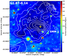
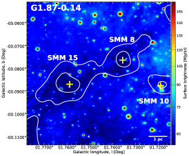
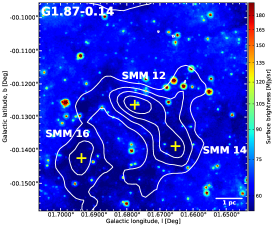
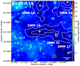
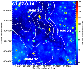
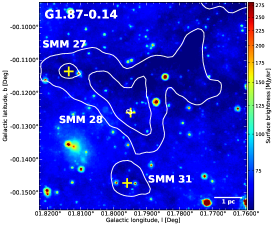
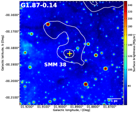
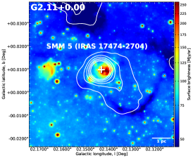
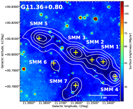
Figure 1: Spitzer/IRAC 8-$\mu$m images of the clumps and filaments studied in the present paper. The images are shown with logarithmic scaling, and the colour bars indicate the surface-brightness scale in MJy sr^-1. The images are overlaid with contours of LABOCA 870-$\mu$m dust continuum emission as in Paper I (starting from $3\sigma$ and going in steps of $3\sigma$, where $3\sigma$ is 0.27, 0.18, 0.12, and 0.14 Jy beam^-1 for the fields G1.87, G2.11, G11.36, and G13.22, respectively). The 870-$\mu$m peak positions of the clumps are denoted by yellow plus signs. In each panel, a scale bar indicating the 1 pc projected length is shown, with the assumption of line-of-sight distance given in Col. (4) of Table LABEL:clumps. The source nomenclature follows that in Paper I. The clumps G1.87–SMM 10, 17, and G13.22–SMM 10 are only partly covered by the MALT90 maps. The white plus sign towards G2.11–SMM 5 shows the position of the UC H ii region from Becker et al. (1994; as seen at 5 GHz) and 18-cm OH maser from Argon et al. (2000); the two positions overlap, and are very close to the 870-$\mu$m peak position.

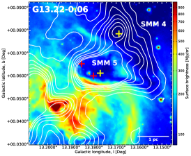
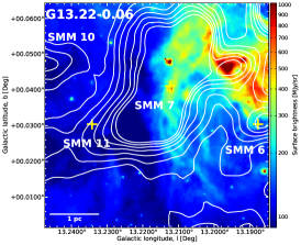
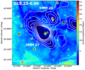
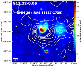
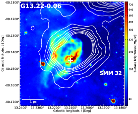
Figure 1: continued. The red plus signs near G13.22–SMM 5 indicate the positions of the 6.7-GHz Class II methanol masers from Szymczak et al. (2000; upper; see also Deharveng et al. (2010)) and Pandian et al. (2008; lower). In the G13.22–SMM 32 panel, the white plus sign marks the position of the compact H ii region from Wink et al. (1982), as observed at 4.9 GHz.

1

Table 1: Characteristics of the LABOCA 870-$\mu$m clumps.

Source	$\alpha_{2000.0}$	$\delta_{2000.0}$	$d$	$R_{\rm eff}$	$M$	$N({\rm H_{2}})$	$\langle n({\rm H_{2}})\rangle$	Comments
	[h:m:s]	[$\degr$:$\arcmin$:$\arcsec$]	[kpc]	[pc]	[M☉]	[$10^{22}$ cm-2]	[$10^{4}$ cm-3]
G1.87-0.14
SMM 1 …	17 49 44.0	-27 33 28	$7.47_{-0.13}^{+0.10}$	$1.50\pm 0.02$	$13\,891\pm 2\,161$	$16.0\pm 2.0$	$50.9\pm 7.9$	IR-dark
SMM 8 …	17 49 59.4	-27 29 24	$7.29_{-0.17}^{+0.13}$	$1.09\pm 0.02$	$2\,679\pm 291$	$5.1\pm 0.8$	$0.9\pm 0.1$	IR-dark
SMM 10 …	17 49 59.7	-27 30 36	$7.28_{-0.18}^{+0.14}$	$0.78\pm 0.02$	$865\pm 102$	$3.1\pm 0.5$	$0.8\pm 0.1$	8 and 24-$\mu$m source
SMM 12 …	17 50 03.0	-27 33 56	$7.32_{-0.17}^{+0.13}$	$1.18\pm 0.02$	$3\,218\pm 351$	$6.5\pm 0.7$	$0.9\pm 0.1$	8 and 24-$\mu$m source
SMM 14 …	17 50 04.2	-27 34 57	$7.40_{-0.15}^{+0.12}$	$0.93\pm 0.02$	$2\,617\pm 285$	$7.7\pm 1.0$	$1.5\pm 0.2$	IR-dark
SMM 15 …	17 50 05.1	-27 28 32	$7.10_{-0.24}^{+0.18}$	$1.00\pm 0.03$	$1\,635\pm 195$	$3.3\pm 0.5$	$0.7\pm 0.1$	group of 8-$\mu$m sources and a 24-$\mu$m source
SMM 16 …	17 50 09.0	-27 33 36	$7.20_{-0.21}^{+0.16}$	$1.15\pm 0.03$	$3\,139\pm 352$	$5.4\pm 0.8$	$0.9\pm 0.1$	IR-dark
SMM 17 …	17 50 12.3	-27 36 48	$7.21_{-0.21}^{+0.16}$	$0.73\pm 0.02$	$1\,506\pm 179$	$5.6\pm 0.8$	$1.8\pm 0.2$	IR-dark
SMM 20 …	17 50 13.5	-27 20 40	$7.00_{-0.26}^{+0.19}$	$1.60\pm 0.05$	$4\,168\pm 499$	$3.8\pm 0.5$	$0.5\pm 0.1$	8 and 24-$\mu$m source
SMM 21 …	17 50 13.8	-27 35 24	$7.21_{-0.21}^{+0.16}$	$0.72\pm 0.02$	$816\pm 76$	$2.9\pm 0.5$	$1.0\pm 0.1$	8 and 24-$\mu$m source
SMM 23 …	17 50 15.0	-27 21 33	$6.98_{-0.27}^{+0.20}$	$1.50\pm 0.05$	$8\,014\pm 969$	$7.4\pm 1.0$	$1.1\pm 0.1$	IR-dark
SMM 24 …	17 50 15.3	-27 34 24	$7.27_{-0.19}^{+0.14}$	$1.15\pm 0.03$	$3\,521\pm 389$	$5.2\pm 0.8$	$1.1\pm 0.1$	IR-dark
SMM 27 …	17 50 18.9	-27 26 32	$7.23_{-0.18}^{+0.14}$	$0.73\pm 0.02$	$1\,266\pm 148$	$4.8\pm 0.8$	$1.5\pm 0.2$	IR-dark
SMM 28 …	17 50 19.2	-27 27 53	$7.03_{-0.26}^{+0.19}$	$1.28\pm 0.04$	$3\,190\pm 380$	$3.8\pm 0.6$	$0.7\pm 0.1$	group of 8-$\mu$m sources and a 24-$\mu$m source
SMM 30 …	17 50 22.8	-27 21 28	$7.02_{-0.25}^{+0.18}$	$1.29\pm 0.04$	$3\,678\pm 434$	$4.1\pm 0.8$	$0.8\pm 0.1$	IR-dark
SMM 31 …	17 50 24.3	-27 28 29	$6.80_{-0.36}^{+0.25}$	$0.66\pm 0.03$	$527\pm 83$	$1.9\pm 0.4$	$0.8\pm 0.1$	8 and 24-$\mu$m source
SMM 38 …	17 50 46.3	-27 24 32	$7.06_{-0.23}^{+0.18}$	$1.33\pm 0.04$	$3\,606\pm 423$	$5.2\pm 0.8$	$0.7\pm 0.1$	IR-dark
G2.11+0.00
SMM 5	17 50 36.0	-27 05 44	$7.40_{-0.12}^{+0.10}$	$1.23\pm 0.02$	$2\,054\pm 215$	$6.9\pm 0.7$	$0.5\pm 0.1$	IRAS 17474-2704; UC H ii region; OH maser;
								extended 8-$\mu$m emission
G11.36+0.80
SMM 1 …	18 07 35.0	-18 43 46	$3.27_{-0.56}^{+0.47}$	$0.38\pm 0.06$	$177\pm 59$	$2.7\pm 0.3$	$1.5\pm 0.5$	8 and 24-$\mu$m source
SMM 2 …	18 07 35.6	-18 43 22	$3.27_{-0.56}^{+0.47}$	$0.37\pm 0.06$	$217\pm 73$	$3.3\pm 0.4$	$2.0\pm 0.7$	IR-dark
SMM 3 …	18 07 35.8	-18 42 42	$3.27_{-0.56}^{+0.47}$	$0.47\pm 0.06$	$255\pm 85$	$3.3\pm 0.4$	$1.1\pm 0.4$	8 and 24-$\mu$m source
SMM 4 …	18 07 36.1	-18 44 26	$3.27_{-0.56}^{+0.47}$	$0.38\pm 0.06$	$140\pm 47$	$2.6\pm 0.3$	$1.2\pm 0.4$	group of 8 and 24-$\mu$m sources
SMM 5 …	18 07 36.7	-18 41 14	$3.27_{-0.56}^{+0.47}$	$0.52\pm 0.08$	$265\pm 89$	$2.7\pm 0.3$	$0.9\pm 0.3$	8 and 24-$\mu$m source
SMM 6 …	18 07 39.0	-18 42 10	$3.27_{-0.56}^{+0.47}$	$0.18\pm 0.03$	$35\pm 13$	$1.4\pm 0.3$	$2.7\pm 1.0$	IR-dark
SMM 7 …	18 07 40.4	-18 43 18	$3.27_{-0.56}^{+0.47}$	$0.34\pm 0.05$	$81\pm 27$	$1.6\pm 0.2$	$0.9\pm 0.3$	8 and 24-$\mu$m source
G13.22-0.06
SMM 4 …	18 13 55.9	-17 28 34	$4.24_{-0.35}^{+0.31}$	$0.93\pm 0.07$	$1\,724\pm 319$	$5.3\pm 0.7$	$1.0\pm 0.2$	8 and 24-$\mu$m source
SMM 5 …	18 14 00.7	-17 28 38	$4.24_{-0.35}^{+0.31}$	$1.08\pm 0.08$	$4\,876\pm 902$	$24.7\pm 2.5$	$1.8\pm 0.3$	8-$\mu$m source and extended 24-$\mu$m emission
SMM 6 …	18 14 08.8	-17 28 57	$4.24_{-0.35}^{+0.31}$	$0.74\pm 0.05$	$920\pm 171$	$3.6\pm 0.5$	$1.0\pm 0.2$	extended 8 and 24-$\mu$m emission
SMM 7 …	18 14 09.4	-17 27 21	$4.24_{-0.35}^{+0.31}$	$1.55\pm 0.11$	$9\,070\pm 1\,678$	$13.3\pm 1.4$	$1.1\pm 0.2$	extended 8 and 24-$\mu$m emission
SMM 10 …	18 14 12.2	-17 25 14	$4.24_{-0.35}^{+0.31}$	$0.53\pm 0.04$	$536\pm 102$	$3.7\pm 0.7$	$1.6\pm 0.3$	IR-dark
SMM 11 …	18 14 14.4	-17 26 30	$4.24_{-0.35}^{+0.31}$	$0.81\pm 0.06$	$767\pm 143$	$2.2\pm 0.4$	$0.7\pm 0.1$	diffuse 8 and 24-$\mu$m emission
SMM 23 …	18 14 36.8	-17 29 22	$3.56_{-0.44}^{+0.39}$	$0.43\pm 0.05$	$252\pm 66$	$2.9\pm 0.4$	$1.4\pm 0.4$	8 and 24-$\mu$m source
SMM 27 …	18 14 40.7	-17 29 22	$3.56_{-0.44}^{+0.39}$	$0.76\pm 0.09$	$1\,757\pm 451$	$13.9\pm 1.5$	$1.8\pm 0.5$	group of 8-$\mu$m sources and a 24-$\mu$m source
SMM 29 …	18 14 42.1	-17 37 06	$12.33_{-0.33}^{+0.38}$	$2.77\pm 0.09$	$17\,927\pm 2\,094$	$10.6\pm 1.1$	$0.4\pm 0.04$	IRAS 18117-1738; extended 8-$\mu$m emission
SMM 32 …	18 14 49.9	-17 32 45	$4.41_{-0.32}^{+0.29}$	$1.33\pm 0.09$	$3\,694\pm 638$	$10.8\pm 1.1$	$0.7\pm 0.1$	H ii region; extended 8-$\mu$m emission

Table 1: continued.

2.2 MALT90 survey data

The spectral-line data of the sources employed in the present study were observed as part of the MALT90 survey (PI: J. M. Jackson; see Foster et al. (2011), 2013; Jackson et al. (2013)). MALT90 observations cover the Galactic longitude ranges $3\degr<l<20\degr$ (1st quadrant) and $300\degr<l<357\degr$ (4th quadrant), and were targeting high-mass star-forming clumps in different stages of evolution. The survey was conducted with the 22-m Mopra telescope in the on-the-fly (OTF) mapping mode during the austral winter in 2010–2012, covering the months of May to October. The OTF mapping was performed with the beam centre scanning in Galactic coordinates $(l,\,b)$ on a $3\aas@@fstack{\prime}4\times 3\aas@@fstack{\prime}4$ grid, where the beam FWHM is $38\arcsec$ at 90 GHz. The scanning speed was $3\aas@@fstack{\prime\prime}92$ s^-1. The step size between adjacent scanning rows was $12\arcsec$, i.e., $\sim 1/3$ of the beam FWHM, resulting in 17 rows per map. Each source was mapped twice by scanning in orthogonal directions ($b$ versus $l$). One map took about half an hour to complete, and the total time spent on each field (two maps) was 1.18 hr. The mapping was carried out when the clump elevation was more than $35\degr$ but less than $70\degr$. The telescope pointing was checked every 1–1.5 hr on SiO maser sources, and was found to be better than $\sim 10\arcsec$.

The spectrometer used was the MOPra Spectrometer (MOPS) which is a digital filter bank. The MOPS spectrometer was tuned to a central frequency of 89.690 GHz, and the 8 GHz wide frequency band of MOPS was split into 16 subbands of 137.5 MHz each (4 096 channels), resulting in a velocity resolution of $\sim 0.11$ km s^-1 in each band (the so-called zoom mode). The typical system temperatures during the observations were in the range $T_{\rm sys}\sim 180-300$ K, and the typical rms noise level is $\sim 250$ mK per 0.11 km s^-1 channel. The output intensity scale given by the Mopra/MOPS system is $T_{\rm A}^{\star}$, i.e., the antenna temperature corrected for the atmospheric attenuation. The observed intensities were converted to the main-beam brightness temperature scale by $T_{\rm MB}=T_{\rm A}^{\star}/\eta_{\rm MB}$, where $\eta_{\rm MB}$ is the main-beam efficiency. The value of $\eta_{\rm MB}$ is 0.49 at 86 GHz and 0.44 at 110 GHz (Ladd et al. (2005)). Extrapolation using the Ruze formula gives the $\eta_{\rm MB}$ values in the range 0.49–0.46 for the 86.75–93.17 GHz frequency range of MALT90.

The 16 spectral-line transitions mapped simultaneously in the MALT90 survey are listed in Table 2. In this table, we give some spectroscopic parameters of the spectral lines, and in the last column we also provide comments on each transition and information provided by the lines. The MALT90 datafiles are publicly available and can be downloaded through the Australia Telescope Online Archive (ATOA).

Table 2: MALT90 spectral-line transitions.

Transition	$\nu$	$E_{\rm u}/k_{\rm B}$	$n_{\rm crit}$	Comments
	[MHz]	[K]	[cm-3]
H13CO${}^{+}(J=1-0)$	86 754.330	4.16	$1.6\times 10^{5}$	high-density and ionisation tracer;
				$J=1-0$ is split into six hyperfine (hf) components
SiO$(J=2-1)$	86 847.010	6.25	$2\times 10^{6}$	shocked-gas/outflow tracer
HN13C$(J=1-0)$	87 090.859	4.18	$2\times 10^{5}$	high-density tracer;
				$J=1-0$ is split into 11 hf components
				with four having a different frequency
C2H$(N_{J,\,F}=1_{3/2,\,2}-0_{1/2,\,1})$	87 316.925	4.19	$2\times 10^{5}$	a tracer of photodissociation regions (PDRs);
				$N_{J}=1_{3/2}-0_{1/2}$ is split into three hf components
HNCO$(J_{K_{a},\,K_{b}}=4_{0,\,4}-3_{0,\,3})$	87 925.238	10.55	$4.5\times 10^{6}$	hot core and shock-chemistry tracer;
				six hf components; $a$-type transition ($\Delta K_{a}=0$)
HNCO$(J_{K_{a},\,K_{b}}=4_{1,\,3}-3_{1,\,2})$	88 239.027	53.86	$2.3\times 10^{6}$	six hf components; $a$-type transition ($\Delta K_{a}=0$)
HCN$(J=1-0)$	88 631.847	4.25	$2.4\times 10^{6}$	high-density and infall tracer;
				$J=1-0$ is split into three hf components
HCO${}^{+}(J=1-0)$	89 188.526	4.28	$1.7\times 10^{5}$	high-density, infall, and ionisation tracer;
				enhanced in outflows due to shock-induced UV radiation
HC13CCN$(J=10-9,\,F=9-8)$	90 593.059	23.91	$1.7\times 10^{5}$	hot-core tracer; five hf components
HNC$(J=1-0)$	90 663.572	4.35	$2.9\times 10^{5}$	high-density tracer; three hf components
13C34S$(J=2-1)$	90 926.036	6.54	$4.3\times 10^{5}$	high-density tracer
HC3N$(J=10-9)$	91 199.796	24.01	$5.3\times 10^{5}$	high-density/hot-core tracer;
				six hf components
CH3CN$(J_{K}=5_{1}-4_{1})$	91 985.316	20.39	$4\times 10^{5}$	hot-core tracer; seven hf components
H$41\alpha$	92 034.475	89.5	$\sim 5$	ionised gas tracer; the principal quantum number
				changes from $n=42$ to 41 $\rightarrow$ $\alpha$-type radio recombination line
13CS$(J=2-1)$	92 494.303	6.66	$5\times 10^{5}$	high-density tracer; three hf components
N2H${}^{+}(J=1-0)$	93 173.480	4.47	$1.5\times 10^{5}$	high-density/CO-depleted gas tracer;
				$J=1-0$ line has 15 hf components out of which
				seven have a different frequency

3 Results and analysis

3.1 Spatial distributions of the spectral-line emission

In this subsection, we present the integrated intensity maps of the spectral lines detected towards the clumps. Besides the maps of integrated intensity, or the 0th moment maps, the MALT90 data archive contains the uncertainty maps of the 0th moment images. The typical $1\sigma$ error, in units of integrated $T_{\rm MB}$, was found to be $\sim 0.6-0.7$ K km s^-1. The HNCO$(4_{1,\,3}-3_{1,\,2})$ maps were an exception, however, as in many cases they were found to be very noisy with $1\sigma$ values of $\sim 3-8$ K km s^-1. Moreover, the HCN and HCO⁺ maps towards G1.87–SMM 38 were corrupted and could not be used.

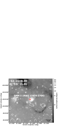
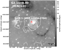
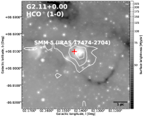
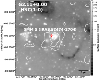
Figure 10: Similar to Fig. 3 but towards G2.11–SMM 5. In each panel, the contour levels start at $3\sigma$, and go in steps of $3\sigma$. The average $1\sigma$ value in $T_{\rm MB}$ units is $\sim 0.68$ K km s^-1. The clump’s LABOCA 870-$\mu$m peak position is marked by a red plus sign. A scale bar indicating the 1 pc projected length is indicated. The HCN, HCO⁺, HNC, and N₂H⁺ show similar clump-like morphologies. The former two species also show an extension to the west of the emission peak.

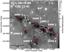
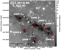
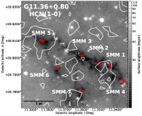
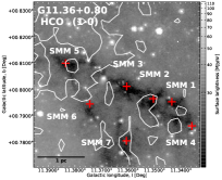
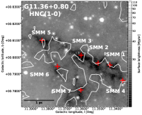
Figure 11: Similar to Fig. 3 but towards the filamentary IRDC G11.36. The contour levels start at $3\sigma$ in all cases except for N₂H⁺, where they start at $5\sigma$. In all cases, the contours go in steps of $3\sigma$. The average $1\sigma$ value in $T_{\rm MB}$ units is $\sim 0.74$ K km s^-1. The LABOCA 870-$\mu$m peak positions of the clumps are marked by red plus signs. A scale bar indicating the 1 pc projected length is indicated. The HCN and HCO⁺ appear to concentrate towards SMM 5, while HNC, and particularly N₂H⁺, are tracing the filamentary 8-$\mu$m absorption feature.

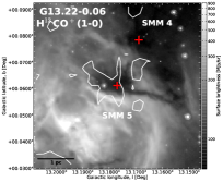
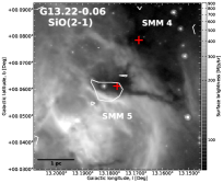
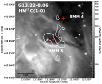
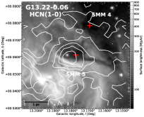
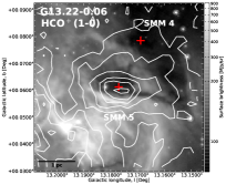
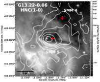
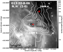
Figure 12: Similar to Fig. 3 but towards G13.22–SMM 4, 5 around the N10/11 IR-bubble pair. The contour levels start at $3\sigma$ for H¹³CO⁺, SiO, HN¹³C, C₂H, and HC₃N, while for HCN, HCO⁺, HNC, and N₂H⁺ they start at $5\sigma$. In all cases, the contours go in steps of $3\sigma$. The average $1\sigma$ value in $T_{\rm MB}$ units is $\sim 0.79$ K km s^-1. The LABOCA 870-$\mu$m peak positions of the clumps are marked by red plus signs. A scale bar indicating the 1 pc projected length is indicated. Note the extended morphological similarities between HCN, HCO⁺, HNC, and N₂H⁺. C₂H shows a ridge-like emission along the northwest-southeast direction. The emission of all the species peaks towards SMM 5.

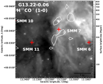
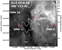
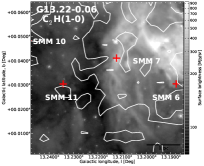
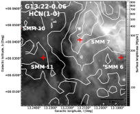
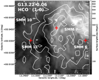
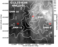
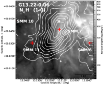
Figure 13: Similar to Fig. 3 but towards G13.22–SMM 6, 7, 10, 11 around the N10/11 bubble. The contour levels start at $3\sigma$ for H¹³CO⁺, HN¹³C, and C₂H, while for HCN, HCO⁺, HNC, and N₂H⁺ they start at $6\sigma$, $6\sigma$, $5\sigma$, and $6\sigma$, respectively. In all cases, the contours go in steps of $3\sigma$. The average $1\sigma$ value in $T_{\rm MB}$ units is $\sim 0.70$ K km s^-1. The LABOCA 870-$\mu$m peak positions of the clumps are marked by red plus signs. The 870-$\mu$m peak of SMM 10 lies just outside the MALT90 map boundary. A scale bar indicating the 1 pc projected length is indicated. Emission from C₂H, HCN, HCO⁺, HNC, and N₂H⁺ are similarly spatially extended, peaking towards SMM 7.

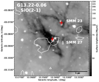
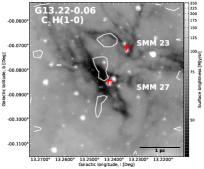
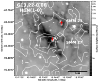
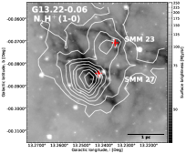
Figure 14: Similar to Fig. 3 but towards G13.22–SMM 23, 27. The contour levels start at $3\sigma$ for H¹³CO⁺, SiO, HN¹³C, C₂H, HNCO$(4_{0,\,4}-3_{0,\,3})$, HCN, and HC₃N, while for HCO⁺, HNC, and N₂H⁺ they start at $5\sigma$, $4\sigma$, and $5\sigma$, respectively. In all cases, the contours go in steps of $3\sigma$. The average $1\sigma$ value in $T_{\rm MB}$ units is $\sim 0.69$ K km s^-1. The LABOCA 870-$\mu$m peak positions of the clumps are marked by red plus signs. A scale bar indicating the 1 pc projected length is indicated. HCN, HCO⁺, HNC, and N₂H⁺ show similar spatial distributions with the emission peaks being well correlated. Although weaker, H¹³CO⁺ and HC₃N also peak near SMM 27.

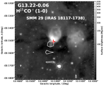
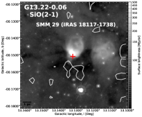
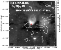
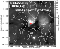
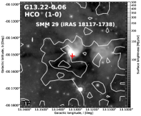
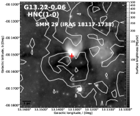
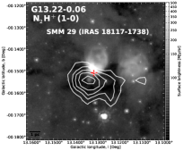
Figure 15: Similar to Fig. 3 but towards G13.22–SMM 29. The contour levels start at $3\sigma$ for H¹³CO⁺, SiO, and C₂H, at $4\sigma$ for HCN and HNC, and at $5\sigma$ for HCO⁺ and N₂H⁺. In all cases, the contours go in steps of $3\sigma$. The average $1\sigma$ value in $T_{\rm MB}$ units is $\sim 0.66$ K km s^-1. The LABOCA 870-$\mu$m peak position of the clump is marked by a red plus signs. A scale bar indicating the 1 pc projected length is indicated. The HCO⁺ and HNC emissions show similar distributions, with HCN sharing some spatial features. The strong N₂H⁺ emission peaks towards the HNC maximum.

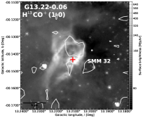
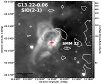
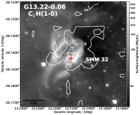
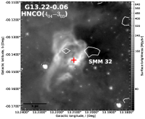
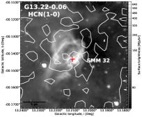
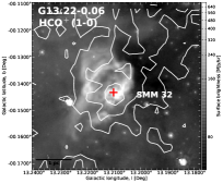
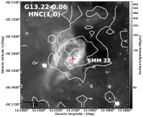
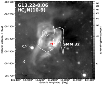
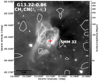
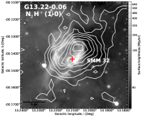
Figure 16: Similar to Fig. 3 but towards G13.22–SMM 32. The contour levels start at $3\sigma$ for H¹³CO⁺, SiO, C₂H, HNCO$(4_{0,\,4}-3_{0,\,3})$, HCN, HC₃N, and CH₃CN, while for HCO⁺, HNC, and N₂H⁺ they start at $4\sigma$, $5\sigma$, and $4\sigma$, respectively. In all cases, the contours go in steps of $3\sigma$. The average $1\sigma$ value in $T_{\rm MB}$ units is $\sim 0.57$ K km s^-1. The LABOCA 870-$\mu$m peak position of the clump is marked by a red plus sign. A scale bar indicating the 1 pc projected length is indicated. The spatial distributions of HCN, HCO⁺, HNC, and N₂H⁺ are quite similar, but note the different peak positions of HCO⁺ and N₂H⁺ (as expected from their chemistry). C₂H and HC₃N also show weaker emission towards SMM 32, with some morphological similarities to the strongly emitting species.

The 0th moment maps are presented in Figs. 3–16 of Appendix B, where the white contours showing the spectral-line emission are overlaid on the Spitzer 8-$\mu$m images. The red plus signs mark the LABOCA peak positions to guide the eye. The line emission was deemed to be real if the integrated intensity was detected at least at the $3\sigma$ level. Only maps of detected line emission are presented. In some cases, the contours are plotted to start at a stronger emission level than $3\sigma$ for illustrative purposes.

As can be seen from Figs. 6 and 13 (cf. Fig. 1), the LABOCA 870-$\mu$m emission peaks of G1.87–SMM 17 and G13.22–SMM 10 are not covered by the MALT90 maps. For most of the lines the detection rate is generally high. In particular, HNC$(1-0)$ and N₂H${}^{+}(1-0)$ were detected towards all fields. Also, SiO$(2-1)$, C₂H$(1_{3/2,\,2}-0_{1/2,\,1})$, HCN$(1-0)$, and HCO${}^{+}(1-0)$ were seen towards $\sim 86-93$% of the fields. As mentioned above, the HNCO$(4_{1,\,3}-3_{1,\,2})$ maps were often very noisy, and emission was not detected even in the cases where the noise level was at the normal level of $0.6-0.7$ K km s^-1. The HC¹³CCN$(10-9)$, H$41\alpha$, and ¹³C³⁴S$(2-1)$ lines were not detected in any of the sources. Moreover, only two fields show weak traces of ¹³C³²S$(2-1)$ emission, which explains the non-detections of the rarer isotopologue ¹³C³⁴S.

3.2 Spectra and line parameters

The beam-averaged ($38\arcsec$) spectra were extracted from the data cubes towards the LABOCA peak positions of the clumps and towards selected line emission peaks. The spectra were analysed using the CLASS90 programme of the GILDAS software package. Linear (first-order) to third-order baselines were determined from velocity ranges without line-emission features, and then subtracted from the spectra. The resulting $1\sigma$ rms noise levels were in the range $\sim 0.2-0.4$ K on the $T_{\rm MB}$ scale. The spectra are presented in Figs. 17–49 of Appendix C. The spectra are overlaid with single Gaussian/hf-structure fits (see below). The coordinates of the line emission peaks in the clump regions are shown in the upper left corners of the corresponding panels (e.g., the HCO⁺ and HNC spectra in Fig. 17). When only weak trace of emission was seen in the 0th moment map, there was no detectable line in the extracted spectrum. This was particularly the case for the ¹³CS$(2-1)$ transition.

As described in Table 2, of the detected lines only SiO$(2-1)$ and HCO${}^{+}(1-0)$ have no hf structure. The SiO and HCO⁺ lines were therefore fitted with a single Gaussian profile using CLASS90. For the rest of the detected lines, we used the hfs method of CLASS90 to fit the hf structure, although the hf components were not fully resolved in any of the sources due to large linewidths typical of massive clumps. The relative positions (in frequency or velocity) and relative strengths of the hf components were searched from the literature (see the references in Table 2) or via the Splatalogue spectral line database. The derived spectral-line parameters are listed in Table LABEL:table:lineparameters at the end of the paper. In Cols. (3) and (4) we give the LSR velocity of the emission (${\rm v}_{\rm LSR}$) and FWHM linewidth ($\Delta{\rm v}$), respectively. Columns (5) and (6) list the peak intensities ($T_{\rm MB}$) and integrated line intensities ($\int T_{\rm MB}{\rm dv}$). The quoted uncertainties in these parameters represent the formal fitting errors (i.e., calibration uncertainties are not taken into account). The values of $T_{\rm MB}$ and $\int T_{\rm MB}{\rm dv}$ were either determined for a blended groups of hf components or, when resolved, for the strongest line which itself could be a multiplet of individual hf lines.

Some of the HCN, HCO⁺, HNC, and N₂H⁺ lines were found to show double-peaked profiles caused by gas kinematics – not by hf splitting. The blue-skewed profiles, i.e., those with blue-shifted peaks stronger than red peaks (e.g., the HCN spectrum towards G1.87–SMM 31; Fig. 31) could be the manifestation of large-scale collapse motions (e.g., Zhou et al. (1993); Myers et al. (1996); Lee et al. (1999); Gao et al. (2009)). In contrast, the red-skewed profiles with stronger red peaks and weaker blue peaks suggest that the envelope is expanding (e.g., Thompson & White (2004); Velusamy et al. (2008); Gao & Lou (2010)); see, for example, the HCN and HNC lines towards G1.87–SMM 1 (Fig. 17). In Table 2, for double-peaked lines we also give the line parameters of both the blue and red peaks separately derived through fitting a single Gaussian to each peak. Finally, in a few cases (e.g., the HCO⁺ line towards G1.87–SMM 1 and G2.11–SMM5) we observe more than one velocity component along the line of sight. These additional velocity components are typically much weaker than the main component and do not significantly contribute to the integrated intensity maps that were constructed by integrating over the whole velocity range.

3.3 Line optical thicknesses and excitation temperatures

The optical thickness of the line emission ($\tau$) and the excitation temperature ($T_{\rm ex}$) could be derived through fitting the hf structure in only some cases. The main reasons for this are the blending of the hf components and limited signal-to-noise (S/N) ratio of the spectra. The average of the $T_{\rm ex}$ values that could be directly derive via the hfs method was adopted for the rest of the given lines. In a few cases we were able to derive the optical thickness by comparing the intensities of two different isotopologues of the same species, namely HCO⁺/H¹³CO⁺ and HNC/HN¹³C [cf. SJF12; their Eq. (6)]. For this analysis, we adopted the galactocentric distance-dependent $[^{12}{\rm C}]/[^{13}{\rm C}]$ ratio from Wilson & Rood (1994):

$$\frac{[^{12}{\rm C}]}{[^{13}{\rm C}]}=7.5\times R_{\rm GC}[{\rm kpc}]+7.6\,.$$ (1)

The optical thickness ratio between the two isotopologues was assumed to be equal to that given by Eq. (1). Using the derived value of $\tau$, the value of $T_{\rm ex}$ was calculated using the familiar antenna equation [see, e.g., Eq. (A.1) of Miettinen (2012a)].

When $T_{\rm ex}$ could not be derived/assumed as described above, we assumed that it is equal to $E_{\rm u}/k_{\rm B}$ in the case of linear molecules (SiO and HC₃N in our case), and that $T_{\rm ex}=2/3\times E_{\rm u}/k_{\rm B}$ in the case of HNCO, which is a nearly prolate asymmetric top molecule, and CH₃CN, which is a prolate symmetric top. These $T_{\rm ex}$ values, used to estimate the line optical thickness, lead to the lower limit to the molecular column density (e.g., Hatchell et al. (1998); see also Miettinen 2012a ). The values of $\tau$ and $T_{\rm ex}$ are listed in Cols. (7) and (8) of Table LABEL:table:lineparameters. In case the line has a hf structure, the $\tau$ value refers to the sum of the peak optical thicknesses of individual hf components. For lines with blended hf multiplets, this total optical thickness was derived by dividing the optical thickness of the strongest hf component by its statistical weight.

3.4 Column densities and fractional abundances

The beam-averaged column densities of the molecules, $N({\rm mol})$, were calculated by using the standard local thermodynamic equilibrium (LTE) formulation:

$$N({\rm mol})=\frac{3h\epsilon_{0}}{2\pi^{2}}\frac{1}{\mu^{2}S}\frac{Z_{\rm rot}(T_{\rm ex})}{g_{K}g_{I}}e^{E_{u}/k_{\rm B}T_{\rm ex}}F(T_{\rm ex})\int\tau({\rm v}){\rm dv}\,,$$ (2)

where $h$ is the Planck constant, $\epsilon_{0}$ is the vacuum permittivity, $\mu$ is the permanent electric dipole moment, $S$ is the line strength, $Z_{\rm rot}$ is the rotational partition function, $g_{K}$ is the $K$-level degeneracy, $g_{I}$ is the reduced nuclear spin degeneracy (see, e.g., Turner (1991)), and $F(T_{\rm ex})\equiv\left(e^{h\nu/k_{\rm B}T_{\rm ex}}-1\right)^{-1}$. Here, the electric dipole moment matrix element is defined as $\left|\mu_{\rm ul}\right|\equiv\mu^{2}S/g_{\rm u}$, where $g_{\rm u}=2J+1$ is the rotational degeneracy of the upper state (Townes & Schawlow (1975)). The values of the product $\mu^{2}S$ were taken from the Splatalogue database. For linear molecules, $g_{K}=g_{I}=1$ for all levels (Turner (1991)). As an asymmetric top, HNCO has $g_{K}=1$ (no $K$-level degeneracy), and due to absence of identical interchangeable nuclei $g_{I}$ is also equal to unity. For the detected CH₃CN line, $g_{K}=2$ because $K\neq 0$ (degeneration among the $K$-type doublets), and $g_{I}=1/4$ because $K\neq 3n$, where $n$ is an integer (Turner (1991)).

The partition function of the linear molecules was approximated as

$$Z_{\rm rot}(T_{\rm ex})\simeq\frac{k_{\rm B}T_{\rm ex}}{hB}+\frac{1}{3}\,,$$ (3)

where $B$ is the rotational constant. The above expression is appropriate for heteropolar molecules at the high temperature limit of $hB/k_{\rm B}T_{\rm ex}\ll 1$. For HNCO, the partition function was calculated as

$$Z_{\rm rot}(T_{\rm ex})=\sqrt{\frac{\pi(k_{\rm B}T_{\rm ex})^{3}}{h^{3}ABC}}\,,$$ (4)

where $A$, $B$, and $C$ are the three rotational constants. For CH₃CN, the partition function is given by Eq. (4) multiplied by $1/3$ due to the three interchangeable H-nuclei (Turner (1991)). We note that for the prolate symmetric top molecule CH₃CN, $B=C$ in Eq. (4).

In case the line profile has a Gaussian shape, the last integral term in Eq. (2) can be expressed as a function of the FWHM linewidth and peak optical thickness of the line as

$$\int\tau({\rm v}){\rm dv}=\frac{\sqrt{\pi}}{2\sqrt{\ln 2}}\Delta{\rm v}\tau\simeq 1.064\Delta{\rm v}\tau\,.$$ (5)

Moreover, if the line emission is optically thin ($\tau\ll 1$), $T_{\rm MB}\propto\tau$, and $N({\rm mol})$ can be computed from the integrated line intensity [see, e.g., Eq. (A.4) of Miettinen (2012a)]. The values of $\tau$ listed in Table 2 were used to decide by which method (from the linewidth or integrated intensity) the column density was computed. Our analysis assumed that the line emission fills the telescope beam, i.e., that the beam filling factor is unity. As can be seen in the 0th moment maps, the line emission is often extended with respect to the $38\arcsec$ ($0\aas@@fstack{\circ}011$) beam size. However, this does not necessarily mean that the assumption of unity filling factor is correct. If the gas has clumpy structure within the beam area, the true filling factor is $<1$. In this case, the derived beam-averaged column density is only a lower limit to the source-averaged value.

The fractional abundances of the molecules were calculated by dividing the molecular column density by the H₂ column density, $x({\rm mol})=N({\rm mol})/N({\rm H_{2}})$. To be directly comparable with the line observations, the $N({\rm H_{2}})$ values were derived from the LABOCA dust continuum maps smoothed to the MALT90 resolution of $38\arcsec$.

The beam-averaged column densities and abundances with respect to H₂ are given in the last two columns of Table LABEL:table:lineparameters. Statistics of these parameters are given in Table 4, where we provide the mean, median, standard deviation (std), and minimum and maximum values of the sample (the values for additional velocity components have been neglected). This table provides an easier way to compare the derived molecular column densities and abundances with those found in other studies.

Table 4: Statistics of column densities and fractional abundances. The notation $a(b)$ means $a\times 10^{b}$.

All clumps
Quantity	Mean	Median	Std	Min.	Max.
$N({\rm H^{13}CO^{+}})$	$7.4(12)$	$6.4(12)$	$2.3(12)$	$5.8(12)$	$1.0(13)$
$x({\rm H^{13}CO^{+}})$	$9.7(-11)$	$1.1(-10)$	$5.1(-11)$	$4.0(-11)$	$1.4(-10)$
$N({\rm SiO})$	$1.9(13)$	$1.5(13)$	$1.3(13)$	$5.5(12)$	$4.8(13)$
$x({\rm SiO})$	$5.7(-10)$	$3.6(-10)$	$5.1(-10)$	$4.0(-11)$	$1.8(-9)$
$N({\rm HN^{13}C})$	$1.1(13)$	$1.1(13)$	$2.5(12)$	$9.6(12)$	$1.5(13)$
$x({\rm HN^{13}C})$	$1.2(-10)$	$1.2(-10)$	$1.6(-11)$	$1.0(-10)$	$1.4(-10)$
$N({\rm C_{2}H})$	$4.3(14)$	$3.4(14)$	$3.3(14)$	$7.8(13)$	$1.2(15)$
$x({\rm C_{2}H})$	$8.1(-9)$	$6.3(-9)$	$6.1(-9)$	$1.8(-9)$	$2.4(-8)$
$N({\rm HNCO})$	$2.2(14)$	$1.4(14)$	$2.2(14)$	$5.4(12)$	$7.9(14)$
$x({\rm HNCO})$	$6.6(-9)$	$5.0(-9)$	$5.8(-9)$	$1.3(-10)$	$1.9(-8)$
$N({\rm HCN})$	$5.9(14)$	$8.7(13)$	$1.4(15)$	$1.6(13)$	$5.5(15)$
$x({\rm HCN})$	$2.1(-8)$	$2.0(-9)$	$5.2(-8)$	$2.7(-10)$	$2.1(-7)$
$N({\rm HCO^{+}})$	$3.0(13)$	$9.7(12)$	$5.6(13)$	$1.1(12)$	$2.6(14)$
$x({\rm HCO^{+}})$	$5.6(-10)$	$3.3(-10)$	$6.9(-10)$	$6.0(-11)$	$3.6(-9)$
$N({\rm HNC})$	$7.1(13)$	$4.8(13)$	$9.4(13)$	$3.7(12)$	$4.4(14)$
$x({\rm HNC})$	$2.2(-9)$	$1.6(-9)$	$2.1(-9)$	$2.3(-10)$	$8.4(-9)$
$N({\rm HC_{3}N})$	$1.6(14)$	$2.8(13)$	$2.8(14)$	$7.0(12)$	$7.9(14)$
$x({\rm HC_{3}N})$	$5.0(-9)$	$6.1(-10)$	$8.5(-9)$	$1.0(-10)$	$2.7(-8)$
$N({\rm CH_{3}CN})$	$5.5(11)$	$5.4(11)$	$1.4(11)$	$4.2(11)$	$7.0(11)$
$x({\rm CH_{3}CN})$	$1.1(-11)$	$1.0(-11)$	$8.1(-12)$	$4.0(-12)$	$2.0(-11)$
$N({\rm N_{2}H^{+}})$	$5.4(13)$	$2.8(13)$	$8.8(13)$	$6.6(12)$	$5.4(14)$
$x({\rm N_{2}H^{+}})$	$1.6(-9)$	$9.9(-10)$	$1.8(-9)$	$2.8(-10)$	$9.8(-9)$
IR-dark clumps
Quantity	Mean	Median	Std	Min.	Max.
$N({\rm SiO})$	$1.5(13)$	$1.1(13)$	$7.9(12)$	$8.2(12)$	$2.8(13)$
$x({\rm SiO})$	$3.6(-10)$	$3.5(-10)$	$1.4(-10)$	$1.6(-10)$	$5.7(-10)$
$N({\rm HN^{13}C})$	$9.6(12)$
$x({\rm HN^{13}C})$	$1.0(-10)$
$N({\rm C_{2}H})$	$4.5(14)$	$1.7(14)$	$4.7(14)$	$7.8(13)$	$1.2(15)$
$x({\rm C_{2}H})$	$8.6(-9)$	$6.3(-9)$	$4.0(-9)$	$5.1(-9)$	$1.3(-8)$
$N({\rm HNCO})$	$2.4(14)$	$1.3(14)$	$2.7(14)$	$5.4(12)$	$7.9(14)$
$x({\rm HNCO})$	$5.5(-9)$	$4.1(-9)$	$5.7(-9)$	$1.3(-10)$	$1.9(-8)$
$N({\rm HCN})$	$6.5(14)$	$2.0(14)$	$7.5(14)$	$3.4(13)$	$1.7(15)$
$x({\rm HCN})$	$2.0(-8)$	$4.4(-9)$	$2.5(-8)$	$9.3(-10)$	$5.6(-8)$
$N({\rm HCO^{+}})$	$2.2(13)$	$1.3(13)$	$2.1(13)$	$1.4(12)$	$6.3(13)$
$x({\rm HCO^{+}})$	$4.3(-10)$	$3.5(-10)$	$3.3(-10)$	$6.0(-11)$	$1.1(-9)$
$N({\rm HNC})$	$9.6(13)$	$6.3(13)$	$1.4(14)$	$3.7(12)$	$5.3(14)$
$x({\rm HNC})$	$2.0(-9)$	$1.7(-9)$	$1.5(-9)$	$4.2(-10)$	$5.5(-9)$
$N({\rm HC_{3}N})$	$1.6(14)$	$3.3(13)$	$3.1(14)$	$1.4(13)$	$7.9(14)$
$x({\rm HC_{3}N})$	$5.1(-9)$	$5.7(-10)$	$1.1(-8)$	$2.8(-10)$	$2.7(-8)$
$N({\rm CH_{3}CN})$	$5.6(11)$	$5.6(11)$	$2.0(11)$	$4.2(11)$	$7.0(11)$
$x({\rm CH_{3}CN})$	$1.2(-11)$	$1.2(-11)$	$1.1(-11)$	$4.0(-12)$	$2.0(-11)$
$N({\rm N_{2}H^{+}})$	$9.0(13)$	$4.0(13)$	$1.6(14)$	$1.6(13)$	$5.4(14)$
$x({\rm N_{2}H^{+}})$	$1.8(-9)$	$1.3(-9)$	$1.5(-9)$	$7.3(-10)$	$5.6(-9)$
IR-bright clumps
Quantity	Mean	Median	Std	Min.	Max.
$N({\rm H^{13}CO^{+}})$	$7.4(12)$	$6.4(12)$	$2.3(12)$	$5.8(12)$	$1.0(13)$
$x({\rm H^{13}CO^{+}})$	$9.7(-11)$	$1.1(-10)$	$5.1(-11)$	$4.0(-11)$	$1.4(-10)$
$N({\rm SiO})$	$2.4(13)$	$2.2(13)$	$1.8(13)$	$5.5(12)$	$4.8(13)$
$x({\rm SiO})$	$9.4(-10)$	$9.7(-10)$	$7.3(-10)$	$4.0(-11)$	$1.8(-9)$
$N({\rm HN^{13}C})$	$1.2(13)$	$1.1(13)$	$2.6(12)$	$1.0(13)$	$1.5(13)$
$x({\rm HN^{13}C})$	$1.3(-10)$	$1.2(-10)$	$1.2(-11)$	$1.2(-10)$	$1.4(-10)$
$N({\rm C_{2}H})$	$4.2(14)$	$4.0(14)$	$2.3(14)$	$1.1(14)$	$8.8(14)$
$x({\rm C_{2}H})$	$7.9(-9)$	$5.2(-9)$	$7.3(-9)$	$1.8(-9)$	$2.4(-8)$
$N({\rm HNCO})$	$1.8(14)$	$1.5(14)$	$1.3(14)$	$1.7(13)$	$4.3(14)$
$x({\rm HNCO})$	$7.9(-9)$	$6.2(-9)$	$5.9(-9)$	$6.1(-10)$	$1.9(-8)$
$N({\rm HCN})$	$5.7(14)$	$6.1(13)$	$1.6(15)$	$1.6(13)$	$5.5(15)$
$x({\rm HCN})$	$2.1(-8)$	$1.7(-9)$	$6.1(-8)$	$2.7(-10)$	$2.1(-7)$
$N({\rm HCO^{+}})$	$3.3(13)$	$9.2(12)$	$6.5(13)$	$1.1(12)$	$2.6(14)$
$x({\rm HCO^{+}})$	$6.2(-10)$	$3.2(-10)$	$8.0(-10)$	$7.0(-11)$	$3.6(-9)$
$N({\rm HNC})$	$7.7(13)$	$3.3(13)$	$1.1(14)$	$4.0(12)$	$4.4(14)$
$x({\rm HNC})$	$2.4(-9)$	$1.4(-9)$	$2.4(-9)$	$2.3(-10)$	$8.4(-9)$
$N({\rm HC_{3}N})$	$1.6(14)$	$2.8(13)$	$2.7(14)$	$7.0(12)$	$7.6(14)$
$x({\rm HC_{3}N})$	$4.7(-9)$	$7.8(-10)$	$7.2(-9)$	$1.0(-10)$	$1.8(-8)$
$N({\rm CH_{3}CN})$	$5.4(11)$
$x({\rm CH_{3}CN})$	$1.0(-11)$
$N({\rm N_{2}H^{+}})$	$4.1(13)$	$2.5(13)$	$3.7(13)$	$6.6(12)$	$1.4(14)$
$x({\rm N_{2}H^{+}})$	$1.5(-9)$	$9.0(-10)$	$1.9(-9)$	$2.8(-10)$	$9.8(-9)$

3.5 Abundance ratios and correlations

As the purpose of the present study is to examine the chemistry of the sources, we computed the abundance ratios between selected molecules. In Table 5, we list the HNC/HCN, HNC/HCO⁺, N₂H⁺/HCO⁺, N₂H⁺/HNC, and HC₃N/HCN column density ratios for the clumps. The quoted uncertainties were propagated from those of the column densities.

We also searched for possible correlations between different parameter pairs. As shown in the upper left panel of Fig. 2, there is a hint that the fractional abundance of HCN decreases as a function of the H₂ column density. A least squares fit to the data points yields $\log\left[x({\rm HCN})\right]=(24.64\pm 13.53)-(1.46\pm 0.60)\log\left[N({\rm H_{2}})\right]$, with the linear Pearson correlation coefficient of $r=-0.55$. For this plot, the H₂ column densities were derived from the LABOCA maps smoothed to the resolution of the MALT90 data. In the rest of the Fig. 2 panels, we show the correlations found between different molecular fractional abundances. The top right panel plots the HCN abundance as a function of $x({\rm HNC})$. The overplotted linear regression model is of the form $\log\left[x({\rm HCN})\right]=(-2.36\pm 3.46)+(0.70\pm 0.39)\log\left[x({\rm HNC})\right]$, with the Pearson’s $r$ of 0.45. The middle left panel plots the HNC abundance as a function of the HCO⁺ abundance. A positive corrrelation is found, and the fitted linear relationship is of the form $\log\left[x({\rm HNC})\right]=(0.42\pm 1.32)+(0.99\pm 0.14)\log\left[x({\rm HCO^{+}})\right]$ ($r=0.80$). The middle right panel shows the HCN abundance plotted as a function of $x({\rm N_{2}H^{+}})$. Again, the data suggest a positive correlation, and the functional form of the linear fit is $\log\left[x({\rm HCN})\right]=(3.56\pm 3.38)+(1.34\pm 0.37)\log\left[x({\rm N_{2}H^{+}})\right]$ ($r=0.71$). The bottom panel shows the HNC abundance as a function of the N₂H⁺ abundance. Here, the correlation coefficient is only 0.39, and no linear fit is shown.

Table 5: Column density ratios.

Source	$\frac{N({\rm HNC})}{N({\rm HCN})}$	$\frac{N({\rm HNC})}{N({\rm HCO^{+}})}$	$\frac{N({\rm N_{2}H^{+}})}{N({\rm HCO^{+}})}$	$\frac{N({\rm N_{2}H^{+}})}{N({\rm HNC})}$	$\frac{N({\rm HC_{3}N})}{N({\rm HCN})}$
G1.87-0.14
SMM 1	…	$8.41\pm 4.13$	$8.57\pm 4.13$	$1.02\pm 0.28$	…
SMM 1	…	$1.83\pm 0.06$	…	…	…
SMM 8	$0.71\pm 0.24$	$2.78\pm 1.08$	$2.00\pm 1.19$	$0.72\pm 0.45$	…
SMM 10	$0.55\pm 0.36$	$8.57\pm 3.62$	$10.00\pm 18.59$	$1.17\pm 2.22$	…
SMM 12	…	$2.84\pm 0.61$	$4.40\pm 8.00$	$1.55\pm 2.84$	…
SMM 14	…	$5.87\pm 1.97$	$3.53\pm 2.41$	$0.60\pm 0.45$	…
SMM 15	…	…	…	$0.11\pm 0.07$	…
SMM 20	…	…	…	$0.09\pm 0.03$	…
SMM 21	…	…	…	$2.05\pm 0.55$	…
SMM 23	$0.24\pm 0.16$	$4.36\pm 2.13$	$3.36\pm 0.48$	$0.77\pm 0.38$	$0.07\pm 0.03$
SMM 23	…	…	…	$1.74\pm 1.15$	…
SMM 24	…	…	…	$0.26\pm 0.19$	…
SMM 27	$0.06\pm 0.03$	…	…	$0.57\pm 0.16$	$0.02\pm 0.01$
SMM 28	$0.01\pm 0.002$	…	…	$1.55\pm 0.34$	$0.02\pm 0.01$
SMM 30	…	$4.36\pm 1.16$	$2.82\pm 0.94$	$0.65\pm 0.26$	…
SMM 31	…	$16.49\pm 6.13$	$2.11\pm 0.31$	$0.13\pm 0.05$	…
SMM 38	…	…	…	$0.69\pm 0.51$	…
SMM 38	…	…	…	$0.48\pm 0.31$	…
G2.11+0.00
SMM 5	$0.25\pm 0.11$	$2.03\pm 0.90$	$1.76\pm 2.59$	$0.87\pm 1.31$	…
G11.36+0.80
SMM 1	…	$5.94\pm 2.19$	$11.25\pm 2.34$	$1.89\pm 0.73$	…
SMM 2	…	$7.14\pm 3.03$	$18.57\pm 3.41$	$2.60\pm 1.08$	…
SMM 3	…	$5.18\pm 1.97$	$10.91\pm 11.09$	$2.11\pm 2.22$	…
SMM 4	…	…	…	$1.15\pm 0.69$	…
SMM 5	…	$1.00\pm 0.26$	$4.25\pm 2.80$	$4.25\pm 2.91$	…
SMM 6	…	$1.68\pm 0.56$	$7.27\pm 12.83$	$4.32\pm 7.64$	…
SMM 7	…	$2.47\pm 0.98$	$2.06\pm 4.07$	$0.84\pm 1.65$	…
G13.22-0.06
SMM 4	$0.21\pm 0.06$	$2.78\pm 0.71$	$3.89\pm 1.01$	$1.40\pm 0.21$	…
SMM 5	$2.86\pm 1.35$	$1.47\pm 0.96$	$0.73\pm 0.40$	$0.50\pm 0.27$	$0.17\pm 0.03$
SMM 6	$0.34\pm 0.13$	$1.36\pm 0.13$	$1.00\pm 0.09$	$0.73\pm 0.36$	…
SMM 7	$6.38\pm 3.05$	$14.23\pm 8.49$	$3.42\pm 1.85$	$0.24\pm 0.11$	…
SMM 7(37 km s-1)	…	$3.67\pm 0.83$	…	…	…
SMM 11	…	$3.02\pm 0.83$	$2.54\pm 2.23$	$0.84\pm 0.77$	…
SMM 11(37 km s-1)	…	$1.07\pm 0.26$	…	…	…
SMM 23	$1.93\pm 2.31$	$5.80\pm 5.86$	$2.00\pm 1.62$	$0.34\pm 0.42$	…
SMM 23(53 km s-1)	…	$1.68\pm 0.34$	…	…	…
SMM 27	$3.67\pm 1.83$	$1.69\pm 1.07$	$0.14\pm 0.08$	$0.08\pm 0.04$	$0.06\pm 0.02$
SMM 29	$0.88\pm 0.43$	$1.52\pm 0.76$	$1.85\pm 0.47$	$1.21\pm 0.52$	…
SMM 29(13.6 km s-1)	…	$1.68\pm 0.43$	…	…	…
SMM 29(37 km s-1)	…	$1.25\pm 0.17$	…	…	…
SMM 29	…	$1.55\pm 1.11$	$2.58\pm 1.44$	$1.67\pm 1.00$	…
SMM 32	$0.47\pm 0.14$	$0.25\pm 0.12$	$0.48\pm 0.26$	$1.94\pm 0.64$	$0.24\pm 0.06$
SMM 32	$0.38\pm 0.11$	$1.40\pm 0.43$	$4.95\pm 1.53$	$3.54\pm 0.77$	…
SMM 32(14 km s-1)	…	$1.83\pm 0.51$	…	…	…

Figure 2: The upper left panel shows the HCN fractional abundance plotted as a function of H₂ column density in logarithmic scales. The rest of the panels show the found correlations between the derived fractional abundances of the molecules. Form top right to bottom panel, the panels plot $x({\rm HCN})$ versus $x({\rm HNC})$, $x({\rm HNC})$ versus $x({\rm HCO^{+}})$, $x({\rm HCN})$ versus $x({\rm N_{2}H^{+}})$, and $x({\rm HNC})$ versus $x({\rm N_{2}H^{+}})$ in logarithmic scales. The solid lines show the least squares fit to the data (see text for details).

4 Discussion

In this section, we discuss the obtained results for each individual species separately. We mostly compare our results with those obtained by VLH11 and SJF12, because they also employed the Mopra telescope observations for their studies.

4.1 HCO⁺ and H¹³CO⁺ (Formylium)

In dense molecular clouds, HCO⁺ is mainly formed through the gas-phase ion-neutral reaction ${\rm H}_{3}^{+}+{\rm CO}\rightarrow{\rm HCO^{+}}+{\rm H}_{2}$ (e.g., Herbst & Klemperer (1973)). The HCO⁺ abundance can be increased in regions where shocks are generated, e.g., due to outflows from embedded YSOs. When the shock heats the gas and produces UV radiation through Ly-$\alpha$ emission ($\lambda=121.6$ nm), the icy grain mantles are evaporated and the HCO⁺ abundance gets enhanced (Rawlings et al. (2000), 2004). This is due to evaporated CO and H₂O, where the latter species can form HCO⁺ in the reaction with photoionised carbon (${\rm C^{+}}+{\rm H_{2}O}\rightarrow{\rm HCO^{+}}+{\rm H}$). The destruction of the HCO⁺ molecules is, in turn, mainly caused by the dissociative recombination with electrons, ${\rm HCO^{+}}+{\rm e}^{-}\rightarrow{\rm CO}+{\rm H}$.

Extended HCO⁺ emission is seen particularly around the submm peaks G1.87–SMM 1, 8, 10, 12, 14–16, and G13.22–SMM 4, 5, 6, 7, 10, 11, 23, 27, and 32. Moreover, the submm clump/UC H ii region G2.11–SMM 5 is associated with an elongated HCO⁺ clump (Fig. 10). In the case of G2.11–SMM 5, G11.36–SMM 5, G13.22–SMM 5, and G13.22–SMM 32, the HCO⁺ emission peak is close to the LABOCA 870-$\mu$m dust emission peak. The clump G1.87–SMM 1 is classified as IR-dark, but the HCO⁺ line towards the submm peak position shows non-Gaussian wing emission, indicative of outflows/shocks. The clumps G13.22–SMM 4–7 and 11 are associated with the Spitzer IR-bubble system N10/11 (Figs. 12 and 13; Churchwell et al. (2006)), which is suggested to represent a site of triggered massive-star formation (Watson et al. (2008)). The strong HCO⁺ emission seen towards the bubble surroundings could originate in the swept-up bubble shells where shock fronts are expanding into the surrounding medium. Moreover, the high-mass stars in the system produce a strong radiation field of UV photons. Some of the IRDCs studied by Liu et al. (2013) show similar extended HCO⁺ emission as the sources studied here. The HCO⁺ column densities derived by Liu et al. (2013), $2.24\times 10^{12}-1.31\times 10^{13}$ cm^-2 ($\sim 5.1\times 10^{12}$ cm^-2 on average), are lower by a factor of about six on average than those we derived. On the other hand, the values derived by SJF12, $5.8\times 10^{13}-1\times 10^{15}$ cm^-2 with the median of $1.88\times 10^{14}$ cm^-2, exceed our values.

The HCO⁺ abundances we derive lie in the range $6\times 10^{-11}-3.6\times 10^{-9}$, with the mean (median) value of $5.6\times 10^{-10}$ ($3.3\times 10^{-10}$). For their sample of the 4th quadrant IRDC sources, VLH11 derived the abundances of $3.5\times 10^{-9}-5.1\times 10^{-8}$ with an average value of $1.7\times 10^{-8}$. Also SJF12 determined higher values of $x({\rm HCO^{+}})$ for their sample of IRDC clumps, ranging from $3.9\times 10^{-9}$ to $2.8\times 10^{-7}$ (with the median of $2.51\times 10^{-8}$). The latter authors found that both the HCO⁺ column density and abundance increase as the clump evolves from the quiescent state with no IR emission (as seen by Spitzer) to “red” state with bright 8-$\mu$m emission and when the central source has likely formed an H ii region. More recently, the MALT90 study of 333 massive clumps by Hoq et al. (2013) revealed a similar evolutionary trend in $x({\rm HCO^{+}})$ (their Fig. 5). We also derive higher HCO⁺ column densities and abundances on average for IR-bright clumps as compared to IR-dark ones, although the median values are quite similar between the two classes. The lowest value of $x({\rm HCO^{+}})$ in our sample is derived towards the IR-dark clump SMM 2 in the G11.36 filament, while the highest abundance is seen towards the IR-bright clump G13.22–SMM 27. The G13.22–SMM 32 clump, associated with an H ii region, also shows a relatively high value of $x({\rm HCO^{+}})$ compared to the rest of our sources. These findings are in agreement with the evolutionary trend found by SJF12. The fact that we derive lower values of $x({\rm HCO^{+}})$ than in VLH11 and SJF12 could mean that our sources are, on average, less evolved. The depletion of CO molecules would, at least partly, explain the meagre amount of HCO⁺ found in the present study. In Paper I, the CO depletion factor was derived towards some of our clumps. For example, towards G11.36–SMM 1 and G13.22–SMM 27 the values $f_{\rm D}({\rm CO})=3.9\pm 0.6$ and $9.9\pm 1.5$ were determined.

The ¹³C isotopologue H¹³CO⁺ is formed in a similar way as the main ¹²C-form except from ¹³CO. The isotope transfer via ${\rm HCO^{+}}+{\rm{}^{13}CO}\leftrightarrow{\rm H^{13}CO^{+}}+{\rm{}^{12}CO}$ can also play a role in the formation of H¹³CO⁺ (Langer et al. (1984)). Only weak emission of H¹³CO⁺, if any, is detected towards our clumps (only three detections). Towards G13.22–SMM 27, the line emission is quite well correlated with the 8-$\mu$m absorption (Fig. 14). The column densities and fractional abundances are derived to be $5.8\times 10^{12}-1\times 10^{13}$ cm^-2 ($7.4\times 10^{12}$ cm^-2 on average) and $4\times 10^{-11}-1.4\times 10^{-10}$ ($9.7\times 10^{-11}$ on average). The former values are comparable to those found by Sakai et al. (2010) for their sample of clumps within IRDCs ($1.3\times 10^{12}-1.4\times 10^{13}$ cm^-2). Vasyunina et al. (2011) derived H¹³CO⁺ abundances of $7.6\times 10^{-11}-7.4\times 10^{-10}$ with an average of $3.4\times 10^{-10}$, which is 3.5 times higher than our average abundance.

4.2 SiO (Silicon Monoxide)

In star-forming regions, SiO emission is usually believed to be linked to the action of high-velocity ($\sim 20-50$ km s^-1) shocks (Martin-Pintado et al. (1992); Schilke et al. (1997); Gusdorf et al. 2008a , b). SiO emission can also trace irradiated medium-velocity ($\sim 10-20$ km s^-1) shocks in PDRs (e.g., Schilke et al. (2001)).

SiO can form via sputtering of Si atoms from the grain cores, which then undergo oxidation through the neutral-neutral gas-phase reactions ${\rm Si}+{\rm O}_{2}\rightarrow{\rm SiO}+{\rm O}$ and ${\rm Si}+{\rm OH}\rightarrow{\rm SiO}+{\rm H}$. If Si is present in the icy grain mantles, a clearly lower shock velocity is sufficient to release it into the gas phase (Gusdorf et al. 2008b ). Alternatively, SiO can be directly formed through dust destruction by vaporisation in grain-grain collisions (e.g., Guillet et al. (2009)). In the hot post-shock gas, OH molecules are abundant due to the reaction ${\rm O}+{\rm H}_{2}\rightarrow{\rm OH}+{\rm O}$. When SiO reacts with OH, a conversion to SiO₂ takes place (${\rm SiO}+{\rm OH}\rightarrow{\rm SiO}_{2}+{\rm H}$; Schilke et al. (1997)). This limits the SiO abundance in the shocked gas.

The SiO emission appears to be quite widespread/extended particularly towards G1.87–SMM 27, 28, 31 (Fig. 8). Moreover, G1.87–SMM 20, 23, 30 (Fig. 7) and G1.87–SMM 38 (Fig. 9) are associated with a few parsec-scale SiO clump. It is also worth noting that the submm peaks G1.87–SMM 28, 30, and 38 are coincident with the local SiO peak positions. Jiménez-Serra et al. (2010) proposed that the extended SiO emission they observed along the filamentary IRDC G035.39-00.33 is the result of a low-velocity shock produced by colliding flows (see also Henshaw et al. (2013)). The widespread SiO emission could therefore originate in the cloud formation process instead of star formation. Sanhueza et al. (2013) recently detected SiO emission from the candidate starless IRDC G028.23-00.19. The authors suggested that the SiO emission with narrow linewidths, coincident with the subclouds’ interface within the source, could be caused by vaporisation of icy grain mantles in grain-grain collisions. Some of our clumps around which extended SiO emission is detected are, however, associated with IR sources, and are likely hosting embedded YSOs. Outflows from these forming stars are likely to be responsible for the detected SiO emission. This is supported by the fact that the SiO and LABOCA emission peaks are coincident in G1.87–SMM 28, 30, and 38, and that some of the line profiles show wing emission. We also note that the filamentary IRDC G11.36 does not show extended SiO emission along its long axis (and neither do the other filaments of this study). The clumps SMM 4 and 5 around the bubble system N10/11 are neither associated with extended SiO emission, although expanding shock fronts are expected to be present there.

Sakai et al. (2010) found that towards their IRDC sources, the SiO column densities are $\sim 4.6\times 10^{12}-3.8\times 10^{13}$ cm^-2 with an average value of $1.5\times 10^{13}$ cm^-2. This is very similar to our clumps, for which $N({\rm SiO})=5.5\times 10^{12}-4.8\times 10^{13}$ cm^-2 ($1.9\times 10^{13}$ cm^-2 on average). However, given the assumption made for $T_{\rm ex}$ (Sect. 3.3), our $N({\rm SiO})$ values should be taken as lower limits. Vasyunina et al. (2011) derived SiO abundances in the range of $1.6\times 10^{-10}-1.6\times 10^{-9}$ (average value $9.5\times 10^{-10}$) towards their IRDCs. Our values, $4\times 10^{-11}-1.8\times 10^{-9}$ (average $5.7\times 10^{-10}$), are mostly comparable to them. Sanhueza et al. (2012) found that the SiO column densities and abundances for their whole sample are $1.36\times 10^{12}-3.47\times 10^{13}$ cm^-2 and $2.78\times 10^{-10}-9.20\times 10^{-10}$ (median values are $7.72\times 10^{12}$ cm^-2 and $5.79\times 10^{-10}$). In particular, their median abundance is close to what we found ($3.6\times 10^{-10}$).

The mean and median SiO abundances are found to be almost three times higher towards IR-bright clumps as compared to IR-dark sources (Table 4), which is in accordance with the results by SJF12. However, there are distinct exceptions from the average SiO trend among our sources, calling its statistical significance into question. The lowest SiO abundance is derived towards the IR-bright clump G13.22–SMM 5, and the second highest SiO abundance is observed towards the IR-dark clump G1.87–SMM 31. Indeed, Sakai et al. (2010) found a trend opposite of ours, and they proposed that the SiO emission from the mid-IR dark sources originates in newly formed shocks, while the SiO emission from more evolved, mid-IR bright sources could originate in gas shocked earlier in time. This could be related to the discovery by Miettinen et al. (2006), namely that the SiO abundance in massive clumps appears to decrease as a function of gas kinetic temperature, possibly reflecting an evolutionary trend.

4.3 HCN, HNC, and HN¹³C [Hydrogen (Iso-)cyanide]

Gas-phase chemical models suggest that HCN and its metastable geometrical isomer, HNC (hydrogen isocyanide), are primarily produced via the dissociative recombination reaction ${\rm HCNH^{+}}+{\rm e^{-}}\rightarrow{\rm HCN}+{\rm H}$ or ${\rm HNC}+{\rm H}$ (e.g., Herbst (1978)). The resulting HNC/HCN abudance ratio is predicted to be 0.9 in this case, i.e., close to unity. The formation of HNC (and only HNC, not HCN) can also take place via the reactions ${\rm H_{2}CN^{+}}+{\rm e^{-}}$ or ${\rm H_{2}NC^{+}}+{\rm e^{-}}\rightarrow{\rm HNC}+{\rm H}$ (Pearson & Schaefer (1974); Allen et al. (1980)). As a result of this additional HNC production channel, the HNC/HCN ratio can rise above unity. Another ways to form HCN and HNC are the neutral-neutral reactions ${\rm CH_{2}}+{\rm N}\rightarrow{\rm HCN}+{\rm H}$ and ${\rm NH_{2}}+{\rm C}\rightarrow{\rm HNC}+{\rm H}$ (Herbst et al. (2000)). After these reactions, the species are able to undergo rapid isomerisation reactions, again leading to the near unity HNC/HCN ratio.

In dense clouds and PDRs, HCN can be photodissociated into CN, either directly or via cosmic-ray induced photodissociation (Boger & Sternberg (2005)). Additional destruction processes of HCN in dense clouds are ${\rm HCN}+{\rm H^{+}}\rightarrow{\rm HCN^{+}}+{\rm H}$ and ${\rm HCN}+{\rm HCO^{+}}\rightarrow{\rm H_{2}CN^{+}}+{\rm CO}$ (Boger & Sternberg (2005)). The HNC molecule can be destroyed via the reactions with hydrogen and oxygen atoms, ${\rm HNC}+{\rm H}\rightarrow{\rm HCN}+{\rm H}$ and ${\rm HNC}+{\rm O}\rightarrow{\rm NH}+{\rm CO}$ (Schilke et al. (1992); Talbi et al. (1996)). HNC also converts to HCN through the reaction ${\rm HNC}+{\rm H^{+}}\rightarrow{\rm HCN}+{\rm H^{+}}$ (Herbst et al. (2000)).

As can be seen in the 0th moment maps in Appendix B, the spatial distributions of HCN and HNC emissions are generally extended. Moreover, for example in the case of G2.11–SMM 5 and G13.22–SMM 5, the submm peak position is close to the peak HCN and HNC emissions. The HN¹³C emission is extended, although weak, in G1.87–SMM 20, 23, 30 (Fig. 7). Similarly, Jackson et al. (2010) found that HNC$(1-0)$ emission traces well the filamentary IRDC G338.4-0.4 or the Nessie Nebula. Sanhueza et al. (2012) found that HNC is ubiquitous in the clumps of IRDCs, in agreement with our results. Also Liu et al. (2013) found a good correlation between the 8-$\mu$m absorption and HNC and HCN emissions towards many of their IRDCs.

The HCN and HNC abundances we derived are in the ranges of $2.7\times 10^{-10}-2.1\times 10^{-7}$ and $2.3\times 10^{-10}-8.4\times 10^{-9}$, respectively. The HN¹³C abundances are found to be $\sim 10^{-10}$ on average. Sakai et al. (2010) found HN¹³C column densities of $\sim 2.6\times 10^{12}-1.4\times 10^{13}$ cm^-2 towards IRDCs, quite similar to our values of $9.6\times 10^{12}-1.5\times 10^{13}$ cm^-2. Vasyunina et al. (2011) derived $x({\rm HCN})$ and $x({\rm HNC})$ values of $3.3\times 10^{-10}-6.8\times 10^{-9}$ (average $2\times 10^{-9}$) and $2.4\times 10^{-10}-6.3\times 10^{-9}$ (average $1.6\times 10^{-9}$), respectively. In general, these are comparable to our values, although the average HCN abundance we found is an order magnitude higher than derived by VLH11. The column densities and fractional abundances of HNC found by SJF12 are $5.1\times 10^{13}-1.36\times 10^{15}$ cm^-2 and $5.1\times 10^{-9}-1.85\times 10^{-7}$. Their median values of $2.42\times 10^{14}$ cm^-2 and $3.73\times 10^{-8}$ are both clearly higher than our values. Among the sample of SJF12, $N({\rm HNC})$ was found to slightly increase with the clump evolution up to the active phase (when the clump shows an extended 4.5-$\mu$m emission and hosts an embedded 24-$\mu$m source), possibly as a result of accretion of the ambient material as suggested by the authors. However, the authors did not found evidence of increasing $x({\rm HNC})$ as a function of source evolution. In contrast, we found higher $N({\rm HNC})$ values towards IR-dark clumps on average than towards IR-bright clumps (the same holds for the median values also). However, the average HNC abundance (but not the median value) appears to be slightly higher in IR-bright clumps.

As shown in the top left panel of Fig. 2, there is a slight hint that $x({\rm HCN})$ decreases when the H₂ column density increases. Although the correlation coefficient is quite low ($r=-0.55$), this could be related to the enhanced abundance of HCO⁺ in more evolved (i.e., denser) sources; HCO⁺ destroys HCN producing H₂CN⁺ ions (see above). The middle left panel of Fig. 2 shows that the HNC abundance increases when the HCO⁺ abundance is enhanced. This can be understood as an increased production of H₂CN⁺ from HCO⁺. The dissociative recombination of H₂CN⁺ then leads to the production of HNC (see above). The top right panel plot of Fig. 2 suggests that the HCN abundance increases when that of HNC increases. This is reminiscent of the positive correlation between the integrated intensities of HCN and HNC found by Liu et al. (2013; their Fig. 17). They also found a similar correlation between HCN and HCO⁺, in agreement with our relationship shown in the middle left panel of Fig. 2. Our positive $x({\rm HCO^{+}})-x({\rm HNC})$ correlation supports the scenario where the HNC abundance increases as the clump evolves. However, if $x({\rm HCN})$ also increases as our Fig. 2 (top right panel) suggests, the possible negative correlation we found between $N({\rm H_{2}})$ and $x({\rm HCN})$ becomes questionable.

The values of the HNC/HCN ratio found towards the clumps lie in the range of $0.01\pm 0.002-6.38\pm 3.05$, with the mean$\pm$std of $1.26\pm 1.78$ (median is 0.47). The average value resembles the result by VLH11 who found that for their IRDCs the HNC/HCN ratio is $\sim 1$. Liu et al. (2013) determined values in the range $0.71\pm 0.11-2.26\pm 0.44$ (average $1.47\pm 0.50$) towards IRDCs, also comparable to our values on average. In the dark cloud cores studied by Hirota et al. (1998), the HNC/HCN ratio was found to be $0.54\pm 0.33-4.5\pm 1.2$ ($2.1\pm 1.2$ on average), mostly comparable to our values within the errors. The above results are consistent with the near unity HNC/HCN ratio theoretically expected in cold molecular clouds (Sarrasin et al. (2010)). However, the abundance ratio between HNC and HCN is strongly dependent on the temperature. A good example is the Orion molecular cloud, where the HNC/HCN ratio was found to strongly decrease (by more than an order of magnitude) when going from the colder quiescent parts of the cloud to the warm plateau and hot-core regions where the ratio is much smaller than unity (Goldsmith et al. (1986); cf. Schilke et al. (1992)). Hirota et al. (1998) found that the HNC/HCN ratio starts to rapidly decrease when the gas kinetic temperature rises above 24 K, because of HNC conversion into HCN. The mean$\pm$std (median) of the HNC/HCN ratio towards our IR-dark clumps is $0.34\pm 0.34$ (0.24), while that for IR-bright clumps is $1.49\pm 1.93$ (0.55). Due to the large scatter of these values, it is difficult to say how well (or poorly) they agree with the earlier studies of the temperature dependence of the HNC/HCN ratio. Moreover, the clump temperatures should be determined in order to study such behaviour more quantitatively. Hoq et al. (2013) examined the integrated intensity ratios between HNC and HCN, and found the median values of 0.9, 0.8, and 0.6 for quiescent IR-dark clumps, clumps containing YSOs, and clumps associated with H ii regions/PDRs. This suggests a possible, although weak, evolutionary trend (see Fig. 4 in Hoq et al. (2013)).

The column density ratio between HNC and HCO⁺ is found to lie in the range $0.25\pm 0.12-16.49\pm 6.13$ with a mean$\pm$std of $4.29\pm 3.94$ (median is 2.78) (the values for the additional velocity components are excluded here). Within the errors, this is in agreement with the gas-phase chemical models of cold dark clouds which suggest comparable abundances for these species (see Roberts et al. (2012) and references therein). Moreover, the average HN¹³C and H¹³CO⁺ abundances, $1.2\times 10^{-10}$ and $9.7\times 10^{-11}$, are very similar. This could be indicative of weak ¹³C fractionation effects. For IR-dark clumps, the mean$\pm$std and median values of the HNC/HCO⁺ ratio are $4.55\pm 2.46$ and 4.36. For IR-bright sources the corresponding values are $4.19\pm 4.47$ and $2.47$. It is therefore possible that the HNC/HCO⁺ ratio decreases slightly as the source evolves. This trend can be seen from the data by SJF12 when the clump evolves from the so-called intermediate state (either extended 4.5-$\mu$m emission or an associated 24-$\mu$m source, but not both) to red state. However, the quiescent sources of SJF12 do not follow this trend.

4.4 C₂H (Ethynyl)

The origin of C₂H in the PDR regions of the interstellar medium, i.e., at the boundary layers between ionised and molecular gas, is believed to be in the photodissociation of acetylene (C₂H₂): ${\rm C_{2}H_{2}}+h\nu\rightarrow{\rm C_{2}H}+{\rm H}$ (e.g., Fuente et al. (1993)). The neutral-neutral reaction ${\rm CH}_{2}+{\rm C}\rightarrow{\rm C_{2}H}+{\rm H}$ can also produce C₂H, where the precursor carbon atom is formed through the photodissociation of CO (e.g., Turner et al. (2000)). The dissociative recombination of the ions CH⁺ (Rimmer et al. (2012)), C₂H${}_{2}^{+}$, and C₂H${}_{3}^{+}$ also yield ethynyl molecules in dense molecular clouds (Mul & McGowan (1980)). The C₂H molecules can themselves be photodissociated back to form C₂ and C₂H⁺ (Fuente et al. (1993)). C₂H is also destroyed through the reactions ${\rm C_{2}H}+{\rm O}\rightarrow{\rm CO}+{\rm CH}$ and ${\rm C_{2}H}+{\rm C^{+}}\rightarrow{\rm C_{3}^{+}}+{\rm H}$ (Watt et al. (1988)).

The spatial distribution of the C₂H emission is found to be quite extended (e.g., the clumps G1.87–SMM 1, G1.87–SMM 20, 23, 30, and G13.22–SMM 32). It is also worth noting that the emission is ridge-like around the IR-bubble pair N10/11 on the side of G13.22–SMM 4 and 5, and extended on the other side containing G13.22–SMM 6, 7, 10, and 11. In N10/11, and towards G13.22–SMM 32, we are probably probing the PDR parts of the sources, where the origin of C₂H can be understood in terms of UV photodissociation. Only weak emission of C₂H is seen towards G1.87–SMM 38, the G11.36 filament, and G13.22–SMM 23, 27, and 29. In the massive star-forming clumps NGC 6334 E and I, both associated with H ii regions, the absence of C₂H emission is suggested to be caused by the destruction of the molecules in such harsh environments (Walsh et al. (2010)). Sanhueza et al. (2013) mapped the IRDC G028.23-00.19 in C₂H, and found the emission to come from the cold central part of the cloud, instead from the outer layers. The authors suggested that C₂H is tracing the dense and cold gas in their IRDC, which seems to be the case also in some of our clumps. Beuther et al. (2008) also found that C₂H is prevalent during the early stages of star formation (and not only in PDRs). They suggested that C₂H starts to decrease in abundance at the hot-core phase due to transformation to other species (e.g., CO from O; see above). Only in the outer layers of the source, where UV photons produce elemental C from CO, the abundance of C₂H can remain high. Furthermore, it was proposed by the authors that C₂H could be a useful tracer of the initial conditions of high-mass star formation.

The C₂H column densities we found, $7.8\times 10^{13}-1.2\times 10^{15}$ cm^-2 ($4.3\times 10^{14}$ cm^-2 on average), are quite similar to those derived by Sakai et al. (2008) towards their IRDC sources ($5.4\times 10^{13}-2.9\times 10^{14}$ cm^-2, the average being $1.5\times 10^{14}$ cm^-2). The fractional abundances we found are $1.8\times 10^{-9}-2.4\times 10^{-8}$ ($8.1\times 10^{-9}$ on average). Similarly to us, VLH11 found abundances in the range $2.5\times 10^{-9}-5.3\times 10^{-8}$ ($1.4\times 10^{-8}$ on average). Sanhueza et al. (2012) derived the values of $6.1\times 10^{13}-7.75\times 10^{14}$ cm^-2 and $7.5\times 10^{-9}-1.62\times 10^{-7}$ for the column densities and abundances of C₂H. Their median column density of $2.41\times 10^{14}$ cm^-2 is similar to our value, but their median abundance of $3.72\times 10^{-8}$ is almost six times higher. We found that both the mean and median values of the C₂H abundance are higher towards IR-dark clumps than towards IR-bright clumps, and the lowest C₂H abundance ($1.8\times 10^{-9}$) is seen towards G13.22–SMM 29, the clump associated with IRAS 18117-1738 and probably (at least) in the hot-core phase of evolution. This is in accordance with the results by Beuther et al. (2008). On the other hand, SJF12 found no clear evolutionary trends for $N({\rm C_{2}H})$ or $x({\rm C_{2}H})$.

4.5 HNCO (Isocyanic Acid)

HNCO is a ubiquitous molecule in the interstellar medium. It was detected for the first time over 40 yr ago in Sgr B2 by Snyder & Buhl (1971). Since then, HNCO has been detected in, e.g., dark clouds (TMC-1; Brown (1981)), low-mass protostellar cores (IRAS 16293-2422; van Dishoeck et al. (1995)), hot cores/UC H ii regions (e.g., G34.3+0.15; MacDonald et al. (1996)), translucent clouds (Turner et al. (1999)), and outflows emanating from massive YSOs (IRAS 17233-3606; Leurini et al. (2011)). Zinchenko et al. (2000) searched for HNCO emission towards a sample of 81 dense molecular cloud cores, and detected it in 57 (70%) of them. Jackson et al. (1984) proposed that HNCO is tracing the densest ($\gtrsim 10^{6}$ cm^-3) parts of molecular clouds. Other authors have suggested that HNCO could be tracing shocks as, for example, it is found to correlate with SiO emission (e.g., Zinchenko et al. (2000); Minh & Irvine (2006); Rodríguez-Fernández et al. (2010)). Association of HNCO clumps with embedded YSOs was recently suggested by the Purple Mountain Observatory 13.7-m telescope observations by Li et al. (2013).

Gas-phase reactions that could be responsible for the formation of HNCO include the dissociative recombinations of H₂NCO⁺ (Iglesias (1977)), H₃NCO⁺, CNH₃O⁺, and CNH₂O⁺, and the neutral-neutral reaction between NCO and H₂ (Turner et al. (1999)). HNCO is dominantly destroyed by reactions with H${}_{3}^{+}$ and He⁺ (Turner et al. (1999)). HNCO could also form through grain-surface chemistry, namely hydrogenation of accreted OCN (Garrod et al. (2008)). In grain ices containing H₂O and NH₃, the HNCO molecules can react with these species to form OCN^- anions (e.g., van Broekhuizen et al. (2004); Table 2 therein). More recently, Tideswell et al. (2010) found that gas-phase reactions are unlikely to be able to produce HNCO in its observed abundances (even at hot-core temperatures). Instead, grain-surface pathways are required, although direct evaporation from the icy grain mantles is not sufficent itself. More complex molecules formed from HNCO on grain surfaces are expected to be evaporated into the gas phase; their dissociation can then lead to the formation of HNCO (Tideswell et al. (2010)).

The HNCO$(4_{0,\,4}-3_{0,\,3})$ emission is found to be extended in many of the clumps (G1.87–SMM 1, 12, 14, 16, 20, 23, 30). Particularly in G1.87–SMM 14, the HNCO emission peaks at the position of the strongest dust emission as traced by LABOCA (Fig. 5). On the other hand, towards G1.87–SMM 20, 23, and 30, where the HNCO emission is also extended, the emission peak is not coincident with any of the submm peaks (Fig. 7). Instead, the HNCO emission has its maximum at the position of the SiO, HNC, HC₃N, CH₃CN, and N₂H⁺ emission maxima. We note that there is no Spitzer 24-$\mu$m source within the Mopra beam in this molecular-line emission peak. Towards G1.87–SMM 1, the HNCO emission morphology is quite similar to that of HC₃N (Fig. 3). Towards the clumps G13.22–SMM 23, 27, and 32 the HNCO emission is very weak (Figs. 14 and 16).

Based on the $4_{0,\,4}-3_{0,\,3}$ transition, the HNCO column densities and fractional abundances are determined to be $5.4\times 10^{12}-7.9\times 10^{14}$ cm^-2 ($2.2\times 10^{14}$ cm^-2 on average) and $1.3\times 10^{-10}-1.9\times 10^{-8}$ ($6.6\times 10^{-9}$ on average). The above values should be taken as lower limits only because of the assumption made for $T_{\rm ex}$ (Sect. 3.3). Vasyunina et al. (2011) derived HNCO abundances of $2.2\times 10^{-10}-3.7\times 10^{-9}$. Their average value, $1.2\times 10^{-9}$, is 5.5 times lower than ours. Sanhueza et al. (2012) found HNCO column densities in the range $\sim 9.8\times 10^{12}-9.9\times 10^{13}$ cm^-2, with the median value of $3.36\times 10^{13}$ cm^-2, i.e., about four times lower than our value ($1.4\times 10^{14}$ cm^-2). The authors found that the column density increases when the source evolves. Our median HNCO column densities agree with this trend, as do the mean and median fractional abundances. It is unclear whether our high $N({\rm HNCO})$ values could point towards more evolved sources on average compared to those studied by SJF12, because the HCO⁺ data suggest the opposite (Sect. 4.1). The fractional HNCO abundances found by SJF12 are $\sim 2.7\times 10^{-10}-7.6\times 10^{-9}$. Their median value, $2.8\times 10^{-9}$, is only $\sim 1.8$ times lower than the value $5\times 10^{-9}$ we found. In most of the clumps studied by SJF12, the HNCO line profiles showed no signatures of shocks. In contrast, we found that eleven of our clumps (G1.87–SMM 1, 8, 10, 14, 15, 21, 24, 27, 28, 31, and 38) show HNCO wing-emission indicative of outflows (and therefore shocks).

4.6 HC₃N and HC¹³CCN (Cyanoacetylene)

Cyanopolyynes are organic chemical species that contain a chain of at least one C-C triple bonds, alternating with single bonds and ending with a cyanide (CN) group. The most simple example of cyanopolyynes is the cyanoacetylene HC₃N. Its first interstellar detection was made towards Sgr B2 (Turner (1971)). This molecule can trace both the cold molecular clouds (see below) and hot cores where it is formed through the gas-phase reaction ${\rm C_{2}H_{2}}+{\rm CN}\rightarrow{\rm HC_{3}N}+{\rm H}$ after C₂H₂ is released from the grain mantles due to heating (e.g., Chapman et al. (2009)).

The HC₃N emission is found to be extended towards many of the observed fields. G1.87–SMM 1 and G1.87–SMM 28 are examples where the line emission peaks towards the dust emission peak. Similarly, Walsh et al. (2010) found that the HC₃N emission closely resembles that of the dust continuum emission in NGC 6334, and suggested that HC₃N is a good tracer of quiescent dense gas (see also Pratap et al. (1997) for the HC₃N emission along the quiescent TMC-1 ridge). The sources G1.87–SMM 20, 23, 30 are associated with a few parsec-scale HC₃N clump, but the line emission peak is not coincident with any of the submm peaks. Instead, the emission morphology resembles those of SiO, HNCO, HNC, and N₂H⁺. Also, the CH₃CN emission towards the field peaks at the HC₃N peak. There is also a small HC₃N clump in G1.87–SMM 38, and its maximum is coincident with the dust peak. The clump G13.22–SMM 5, belonging to the N10/11 bubble system, is associated with a small HC₃N clump. On the other hand, towards G1.87–SMM 8, 10, 14–17, 21, 24, and G13.22–SMM 23, 27 the HC₃N emission is very weak or absent. The HC₃N line wings detected towards some of our clumps suggest the shock-origin for the emission (e.g., the case of the IR-dark clump G1.87–SMM 27)

The HC₃N column densities and abundances we derive are $7\times 10^{12}-7.9\times 10^{14}$ cm^-2 and $1\times 10^{-10}-2.7\times 10^{-8}$. The mean values are $1.6\times 10^{14}$ cm^-2 and $5\times 10^{-9}$. Similarly to the linear SiO molecule, we assumed that $T_{\rm ex}=E_{\rm u}/k_{\rm B}$ (Sect. 3.3), so the above values should be interpreted as lower limits. Sakai et al. (2008) determined $N({\rm HC_{3}N})$ values in the range $<2.2\times 10^{12}-5.4\times 10^{13}$ cm^-2 for their sources. Our mean column density exceeds the highest value found by Sakai et al. (2008) by a factor of three. Vasyunina et al. (2011) derived HC₃N abundances of $1\times 10^{-10}-1.5\times 10^{-9}$ with an average value of $5.4\times 10^{-10}$. Our average value is almost an order of magnitude higher. The $N({\rm HC_{3}N})$ values derived by SFJ12 are $1.4\times 10^{12}-3.33\times 10^{13}$ cm^-2 (median $4.77\times 10^{12}$ cm^-2). Their median $N({\rm HC_{3}N})$ is about six times lower than ours but the median abundance for their sample, $4.23\times 10^{-10}$, is comparable to our value of $6.1\times 10^{-10}$.

In agreement with the chemical model by Nomura & Millar (2004), SJF12 found that $N({\rm HC_{3}N})$ increases as a function of clump evolutionary stage, but their median abundances did not show such a trend. Among the quiescent clumps they studied, HC₃N was detected in only one source. The trend between $N({\rm HC_{3}N})$ and evolutionary stage found by SJF12 is not seen among our sources. On the other hand, we found that the average HC₃N abundance is very similar between the IR-dark and -bright clumps ($5.1\times 10^{-9}$ and $4.7\times 10^{-9}$), while the median value is about 1.4 times higher towards the latter sources.

The HC₃N/HCN ratios are found to lie in the range $0.02\pm 0.01-0.24\pm 0.06$, where the mean$\pm$std is $0.10\pm 0.09$ (median is 0.07). For comparison, Dickens et al. (2000) found that the HC₃N/HCN ratio is about 0.05–0.07 in the L134N (L183) prestellar core. In comet Hale-Bopp, the above ratio is found to be 8.2% (Bockelée-Morvan et al. (2000)). More recently, Chapillon et al. (2012), who made the first detection of HC₃N in protoplanetary disks, derived the HC₃N/HCN ratios of $\leq 0.05$, 0.075, and 0.55 towards DM Tau, LkCa 15, and MWC 480, respectively. Interestingly, the abundance ratio between HC₃N and HCN appears to be quite similar in IRDC clumps, low-mass prestellar cores, disks around T Tauri stars, and comets.

The ¹³C isotopologue of HC₃N, HC¹³CCN, forms via the isotope exchange reaction ${\rm{}^{13}C^{+}}+{\rm HC_{3}N}\rightarrow{\rm C^{+}}+{\rm HC^{13}CCN}$ (Takano et al. (1998)). No HC¹³CCN emission was detected in any of our sources. The $E_{\rm u}/k_{\rm B}$ value of the observed HC¹³CCN transition is very similar to that of HC₃N ($\sim 24$ K), so the non-detection is not likely to be caused by excitation conditions. The probable reasons are the relative rareness of HC¹³CCN, and the limited S/N ratio of mapping observations. A positive detection is expected with a longer integration time/single-pointing observation, at least towards the strongest HC₃N sources. HC¹³CCN was first detected in Sgr B2 by Gardner & Winnewisser (1975), and Gibb et al. (2000) make a detection towards the hot core G327.3-0.6.

4.7 ¹³CS and ¹³C³⁴S (Carbon Monosulfide)

Only traces of ¹³CS$(2-1)$ emission are seen towards the clump G1.87–SMM 1 (Fig. 3), and towards the field containing G1.87–SMM 27, 28, and 31 (Fig. 8). ¹³C³⁴S is not detected at all. Beuther & Henning (2009) found only weak ¹³CS$(2-1)$ emission towards the IRDCs 19175-4 and -5, and derived very high CS depletion factors of $\sim 100$. Although CS can suffer from depletion onto dust grain surfaces in cold sources, its non-detection in the present study is likely caused by limited S/N ratio. Also VLH11 detected only very weak ¹³CS$(2-1)$ emission in only three sources of their IRDC sample, with an average $x({\rm{}^{13}CS})$ of $3\times 10^{-10}$.

4.8 CH₃CN (Methyl Cyanide)

Methyl cyanide is a good tracer of warm/hot and dense parts of molecular clouds (e.g., Araya et al. (2005); Purcell et al. (2006)). The formation of CH₃CN is likely taking place on the grain surfaces during the earliest stages of YSO evolution. The most efficient route for this is the reaction between CH₃ and CN (e.g., Garrod et al. (2008)). Later, when the central star starts to heat its surrounding medium, CH₃CN gets evaporated into the gas phase. In the gas phase, CH₃CN can form when CH${}_{3}^{+}$ and HCN first form H₄C₂N⁺ ions through radiative association, and which then dissociatively recombine with electrons to form CH₃CN molecules and H-atoms (e.g., Mackay (1999)). Shocks associated with YSO outflows can also be responsible for the production of CH₃CN (Codella et al. (2009)). The CH₃CN molecules can be photodissociated into CH₃ and CN molecules (Mackay (1999)).

Inspection of the CH₃CN maps shows that the emission is quite weak in most cases (e.g., G1.87–SMM 12, 14, 16, 27, 28, and 31). Towards G1.87–SMM 1, the CH₃CN emission is extended (although weak) around the submm peak (Fig. 3). Interestingly, the clump appears to be IR-dark, so perhaps the emission has its origin in shocks. Between the submm peaks G1.87–SMM 20, 23, and 30, there is a pc-scale CH₃CN clump, with the emission peak being coincident with the SiO, HNCO, HNC, HC₃N, and N₂H⁺ maxima (Fig. 7). Also here, the shock-origin of CH₃CN is supported by the coincidence with the SiO and HNCO emission peaks.

The CH₃CN column densities and fractional abundances could be derived only towards three positions (where the extracted spectra showed visible lines). These are $5.5\times 10^{11}$ cm^-2 and $\sim 10^{-11}$ on average. These are only lower limits because we assumed that $T_{\rm ex}=2E_{\rm u}/3k_{\rm B}$ (Sect. 3.3). Beuther & Sridharan (2007) found an order of magnitude higher average values for both the column density and abundance towards their IRDC sources. However, they used single-pointing observations with the IRAM 30-m telescope, while we have used OTF-data with lower S/N ratios. It is also possible that our sources are in an earlier stage of evolution and therefore show only weak CH₃CN emission. For example, Nomura & Millar (2004) modelled the chemistry of the hot core G34.3+0.15, and found that the CH₃CN column density is at the level we have derived when the source’s age is only $\lesssim 10^{3}$ yr. Moreover, Vasyunina et al. (2011) detected no CH₃CN emission towards their IRDCs, and SJF12 found CH₃CN emission in only one active (extended 4.5-$\mu$m emission in addition to a YSO seen at 24 $\mu$m) clump (G034.43 MM1) of their large sample of IRDC sources. The hot cores studied by Bisschop et al. (2007) show CH₃CN abundances of $1.5\times 10^{-8}-1.5\times 10^{-7}$, much higher than seen towards IRDCs.

4.9 H41$\alpha$

The H41$\alpha$ recombination line emission is not detected in this study. It is known that some of our clumps do contain H ii regions, and in these partially or fully ionised gas regions protons can capture electrons. Therefore, these H ii regions are expected to emit recombination lines. The non-detection towards the clumps with H ii regions is likely caused by our low S/N ratio (similarly to HC¹³CCN and ¹³CS). For example, Araya et al. (2005), who used single-pointing 15-m SEST telescope observations, detected H41$\alpha$ line emission in nine sites of high-mass star formation. More recently, Klaassen et al. (2013) detected H41$\alpha$ towards the high-mass star-forming region K3-50A using the CARMA interferometer, and suggested that the line is tracing the outflow entrained by photoionised gas.

4.10 N₂H⁺ (Diazenylium)

Due to its resistance of depletion at low temperatures and high densities, N₂H⁺ is an excellent tracer of cold and dense molecular clouds (e.g., Caselli et al. (2002)). Diazenylium molecules are primarily formed through the gas-phase reaction ${\rm H_{3}^{+}}+{\rm N_{2}}\rightarrow{\rm N_{2}H^{+}}+{\rm H_{2}}$. When there are CO molecules in the gas phase, they can destroy N₂H⁺ producing HCO⁺ (${\rm N_{2}H^{+}}+{\rm CO}\rightarrow{\rm HCO^{+}}+{\rm N_{2}}$). When CO has depleted via freeze-out onto dust grains, N₂H⁺ is mainly destroyed in the electron recombination (${\rm N_{2}H^{+}}+{\rm e^{-}}\rightarrow{\rm N_{2}}+{\rm H}$ or ${\rm NH}+{\rm N}$).

The N₂H⁺ emission is found to be extended towards many of our fields (e.g., the fields covering G1.87–SMM 1; G1.87–SMM 12, 14, 16; G1.87–SMM 20, 23, 30; G1.87–SMM 27, 28, 31; G1.87–SMM 38; G13.22–SMM 23, 27; G13.22–SMM 32). The N₂H⁺ emission is also tracing well the G11.36 filament as seen by LABOCA at 870 $\mu$m and in absorption by Spitzer at 8 $\mu$m (Fig. 11). Very strong and extended N₂H⁺ emission is seen around the N10/11 double bubble, and the emission peaks are coincident with the submm peaks G13.22–SMM 5 and 7 (Figs. 12 and 13). Also in G1.87–SMM 38 the line emission peaks at the dust peak (Fig. 9). Interestingly, towards G1.87–SMM 20, 23, 30, the N₂H⁺ emission peaks in between the submm dust emission maxima, where also line emission from several other species has its maximum as discussed earlier. Also in G13.22–SMM 23, 27, and 32 the N₂H⁺ emission peaks are offset from the submm peaks by $17\arcsec$, $15\aas@@fstack{\prime\prime}9$, and $30\aas@@fstack{\prime\prime}5$, respectively. The pc-scale N₂H⁺ clump in G2.11–SMM 5 has its maximum about $11\aas@@fstack{\prime\prime}6$ (0.42 pc) in projection from the strongest dust emission. Ragan et al. (2006) and Liu et al. (2013), who mapped IRDCs in the $J=1-0$ line of N₂H⁺, also found good correspondence between the line emission and 8-$\mu$m absorption.

We found N₂H⁺ column densities in the range of $6.6\times 10^{12}-5.4\times 10^{14}$ cm^-2, and abundances of $2.8\times 10^{-10}-9.8\times 10^{-9}$. The average values are $5.4\times 10^{13}$ cm^-2 and $1.6\times 10^{-9}$, respectively. Ragan et al. (2006) derived comparable abundances of $5.7\times 10^{-11}-2\times 10^{-9}$ for their sample of IRDCs. The column density range found by Sakai et al. (2008) for their IRDCs, $\sim 4.3\times 10^{12}-1.3\times 10^{14}$ cm^-2, is also very similar to our range of values. Vasyunina et al. (2011) derived fractional N₂H⁺ abundances of $1.9\times 10^{-10}-8.5\times 10^{-9}$ with an average of $2.8\times 10^{-9}$, remarkably similar to our values. More recently, SJF12 derived column densities of $3.6\times 10^{12}-1.37\times 10^{14}$ cm^-2 (median is $1.6\times 10^{13}$ cm^-2) and abundances in the range $1.9\times 10^{-10}-1.68\times 10^{-8}$ (the median being $2.4\times 10^{-9}$), again similar to our results. They also found that both the values of $N({\rm N_{2}H^{+}})$ and $x({\rm N_{2}H^{+}})$ increase as the clump evolves from quiescent (IR-dark) to star-forming stage. Similarly, Hoq et al. (2013) found that $x({\rm N_{2}H^{+}})$ rises as a function of evolutionary stage (their Fig. 5). The reason for such a correlation is somewhat unclear because of the destroying effect of CO (see above), and in contrast, our clumps show the opposite trend. Sanhueza et al. (2012) suggested that the rate coefficients of the relevant chemical reactions might be inaccurate, and/or the large beam size of Mopra observations is seeing the cold N₂H⁺ gas around the warmer central YSOs, thus leading to their observed correlation. On the other hand, higher temperature could lead to an enhanced evaporation of N₂ from the dust grains, thus allowing N₂H⁺ to increase in abundance (Chen et al. (2013)). Finally, Liu et al. (2013) derived N₂H⁺ column densities of $\sim 3.3\times 10^{12}-2.7\times 10^{13}$ cm^-2 with the mean value being $\sim 9.4\times 10^{12}$ cm^-2 – a factor of about six lower than ours.

The N₂H⁺/HCO⁺ ratios we derived lie in range $0.14\pm 0.08-18.57\pm 3.41$, i.e., the ratio varies a lot. The mean$\pm$std is $4.48\pm 4.26$, and the median value is 3.36. Separately for IR-dark and -bright clumps, these values are $6.59\pm 5.82$ and 3.53, and $8.49\pm 22.61$ and 2.54, respectively. Due to the large dispersion in these values, there is no clear correlation between the clump evolutionary stage and the value of the N₂H⁺/HCO⁺ ratio among our source sample. However, one would expect to observe a higher ratio of N₂H⁺/HCO⁺ towards clumps in the earliest stages of evolution, which is actually mildly suggested by our median values. This is because CO is expected to be depleted in starless clumps, so that HCO⁺ cannot form via the reaction between ${\rm H_{3}^{+}}$ and ${\rm CO}$. When the source evolves, it gets warmer and CO should be evaporated from the dust grains when the dust temperature exceeds about $\sim 20$ K (see Tobin et al. (2013)). Two effects can then follow: the CO molecules can start to form HCO⁺, and destroy N₂H⁺. As a consequence, the N₂H⁺/HCO⁺ ratio should decrease. Sanhueza et al. (2012) indeed found that the N₂H⁺/HCO⁺ abundance ratio decreases from intermediate to active and red clumps, and therefore acts as a chemical clock in accordance with the scenario described above. However, the quiescent clumps studied by SJF12 do not follow this trend. As an explanation for this, the authors suggested, for example, that some of them could contain YSOs not detected by Spitzer, or that CO has not had enough time to deplete from the gas phase. During the starless phase of evolution, however, the N₂H⁺/HCO⁺ ratio is expected to increase (CO gets more and more depleted and cannot destroy N₂H⁺). Hoq et al. (2013) also inspected whether there is an evolutionary trend in the N₂H⁺/HCO⁺ abundance ratio, and the median value appeared to be slightly higher in more evolved clumps, although, as the authors stated, the result is not statistically significant (their Fig. 6). Hoq et al. (2013) employed the chemical evolution model by Vasyunina et al. (2012) to further investigate the behaviour of the N₂H⁺/HCO⁺ ratio. As shown in their Fig. 10, the abundance ratio appears to increase as a function of time until the peak value is reached at $\sim 10^{4}$ yr.

We also derived the N₂H⁺/HNC ratios, ranging from $0.08\pm 0.04$ to $4.32\pm 7.64$. The mean$\pm$std is $1.26\pm 1.07$, and the median value is 0.87. For IR-dark clumps these values are $1.20\pm 1.17$ and 0.72, while for IR-bright clumps they are $1.26\pm 1.05$ and 1.17. The median N₂H⁺/HNC ratio found by SJF12 for all their clumps (0.07) is comparable to the lowest values we found, while our median is over 12 times higher. For the IRDC sample examined by Liu et al. (2013), the ratio ranges from $\sim 0.54-3.86$ with the mean$\pm$std of $1.20\pm 0.79$ and median of 1.07 (computed from the values in their Table 4). These are comparable with our values. Sanhueza et al. (2012) suggested that there is a trend of increasing N₂H⁺/HNC ratio with the clump evolution, but the change in their median value is very small, only from 0.06 for quiescent clumps to 0.08 for active and red clumps. Our clumps show a similar, except stronger, trend in median values (also the average ratios suggest this trend). Sanhueza et al. (2012) proposed that HNC could be preferentially formed during the cold phase, while their median N₂H⁺ abundance appeared to increase when the source evolves. We found that there is a positive N₂H⁺ – HCN abundance correlation, as shown in the middle right panel of Fig. 2. A weaker, although possible positive correlation, is also found between N₂H⁺ and HNC (Fig. 2, bottom panel). Accoring to our and Liu et al. (2013) results, the N₂H⁺/HNC ratio is near unity on average, although the std is very large. If the increasing trend in $x({\rm HNC})$ as a function of $x({\rm N_{2}H^{+}})$ is real, the abundance ratio is not expected to change significantly, which conforms to the results by SJF12 and of the present study.

5 Summary and conclusions

Altogether 14 subfields from the LABOCA 870-$\mu$m survey of IRDCs by Miettinen (2012b) are covered by the MALT90 molecular-line survey. These IRDC fields contain 35 clumps in total, ranging from quiescent (IR-dark) sources to clumps associated with H ii regions. In the present study, the MALT90 observations were used to investigate the chemical properties of the clumps. Our main results and conclusions are summarised as follows:

1. Of the 16 transitions at $\lambda\approx 3$ mm included in the MALT90 survey, all except five [HNCO$(4_{1,\,3}-3_{1,\,2})$, HC¹³CCN$(10-9)$, ¹³C³⁴S$(2-1)$, H$41\alpha$, ¹³CS$(2-1)$] are detected towards our sources.

2. The HCO${}^{+}(1-0)$ emission is extended in many of the clumps, resembling the MALT90 mapping results of IRDCs by Liu et al. (2013). The fractional HCO⁺ abundances appear to be lower than in the IRDC clumps studied by Vasyunina et al. (2011) and Sanhueza et al. (2012), who also used the Mopra telescope observations. We found that the average HCO⁺ abundance increases when the clump evolves (the median HCO⁺ abundance is very similar between the IR-dark and -bright clumps), resembling the trend discovered by Sanhueza et al. (2012) and Hoq et al. (2013). The H¹³CO${}^{+}(1-0)$ emission is generally weak in our clumps, and its average abundance is a factor of 3.5 lower than in the sources of Vasyunina et al. (2011).

3. Extendend or clump-like SiO$(2-1)$ emission is seen towards several clumps. In three cases, the maximum of the integrated intensity of SiO is coincident with the LABOCA 870-$\mu$m peak position. As supported by the observed line wings, SiO emission is likely caused by outflow activity which generates shocks releasing SiO into the gas phase. However, some of the widespread SiO emission could result from shocks associated with cloud formation as suggested in the IRDC G035.39-00.33 (Jiménez-Serra et al. (2010)). The SiO abundances derived for our clumps are mostly comparable to those seen in other IRDCs (Vasyunina et al. (2011); Sanhueza et al. (2012)). No trend of decreasing SiO abundance with the clump evolution is seen, as suggested by some earlier studies of massive clumps (Miettinen et al. (2006); Sakai et al. (2010)). Instead, our data suggest the opposite trend, as seen in the data by Sanhueza et al. (2012).

4. The $J=1-0$ line emission of HCN and HNC is generally found to be spatially extended. The fractional abundances of these species are mostly comparable to those found by Vasyunina et al. (2011), but Sanhueza et al. (2012) derived clearly higher HNC abundances. We found no evidence of increasing HNC column density as the source evolves as the latter authors did. However, our average HNC abundance (but not the median value) appears to be slightly higher in more evolved sources. This is perhaps related to the accumulation of gas from the surrounding mass reservoir (Sanhueza et al. (2012)). We found a hint that the HCN abundance gets lower when the column density of molecular hydrogen becomes higher. This might be related to the enhanced HCO⁺ abundance in more evolved sources, where the species can destroy HCN molecules to form H₂CN⁺ and CO. The HNC abundance is found to increase as a function of the HCO⁺ abundance. This is likely related to the increased production of H₂CN⁺ – a molecular ion that forms HNC in the dissociative recombination with an electron. The HCN fractional abundance appears to increase when that of HNC increases, in agreement with the result by Liu et al. (2013). In this case, however, the decrease in $x({\rm HCN})$ as a function of time is questionable, if HNC gets more abundant as the clump evolves. The HNC/HCN ratio is found to lie in the range $\sim 0.01-6.38$ with an average value near unity, as seen in other IRDCs (Vasyunina et al. (2011); Liu et al. (2013)). It is also in agreement with the theoretical prediction (Sarrasin et al. (2010)). The gas kinetic temperature measurements would be needed to study how the HNC/HCN ratio depends on the temperature. Moreover, the average HNC/HCO⁺ and HN¹³C/H¹³CO⁺ ratios, $\sim 4.3\pm 3.9$ and $\sim 1.8\pm 1.1$, are in reasonable agreement with the gas-phase chemical models which suggest similar abundances for HNC and HCO⁺ and their ¹³C isotopologues in the case of weak ¹³C fractionation (see, e.g., Roberts et al. (2012) and references therein). The median HNC/HCO⁺ ratio is found to decrease as the clump evolves, in agreement with data from Sanhueza et al. (2012).

5. The C₂H$(N=1-0)$ emission is also found to be extended. This molecule is believed to be a good tracer of the PDR regions. Towards the IR-binary bubble system N10/11 and the clump G13.22–SMM 32, the detected extended C₂H emission is likely related to the UV photodissociation process. Recently, C₂H is found to trace cold gas in the IRDC G028.23-00.19 by Sanhueza et al. (2013), and this also appears to be the case in some of our sources. The fractional C₂H abundances are found to be comparable with the values obtained by Vasyunina et al. (2011), but the median abundance derived by Sanhueza et al. (2012) exceeds our value by a factor of $\sim 6$. We found that the average and median C₂H abundances are lower towards more evolved clumps, some of which are likely to be in the hot-core phase or even more evolved. This agrees with the suggestion that C₂H starts to decrease in abundance in hot cores, and could therefore be used to probe the initial conditions of massive-star formation (Beuther et al. (2008)).

6. The HNCO$(4_{0,\,4}-3_{0,\,3})$ line emission shows extended morphology towards many of our sources. The average HNCO abundance we derive is a factor of 5.5 times higher than the value obtained by Vasyunina et al. (2011). However, the median value we found is comparable to the one derived by Sanhueza et al. (2012) (within a factor of $\sim 1.8$). According to models, grain-surface chemistry appears to be required for the origin of gas-phase HNCO (Tideswell et al. (2010)). The extended-like emission of HNCO could have its origin in shocks, as suggested in some other molecular clouds (e.g., Zinchenko et al. (2000)). In some cases, this is supported by the similarity to the SiO emission, and also by non-Gaussian line wing emission. Our HNCO data support the discovery that the molecule’s column density increases as the clump evolves (Sanhueza et al. (2012)); also the fractional abundance shows such a trend in the present study.

7. The $J=10-9$ emission of cyanoacetylene (HC₃N) shows extended morphology towards many of our clumps. In some cases the emission maxima correlate well with the dust emission peaks. However, in some sources the HC₃N emission is found to be weak or completely absent. The deteced line wings suggest that the HC₃N emision has its origin in shocks. On average, we derived an order of magnitude higher abundance of HC₃N than what Vasyunina et al. (2011) determined for their sources. Our median HC₃N abundance is very close to that derived by Sanhueza et al. (2012; within a factor of $\sim 1.4$). The latter authors found that the column density of HC₃N increases as the clump evolves, but our column density data do not show such a trend. Only the median abundance shows a hint of positive correlation with the clump evolution. Our results support the finding that, besides tracing hot cores, HC₃N can also exist in cold molecular clouds (e.g., in the prestellar core L183; Dickens et al. (2000)). The HC₃N/HCN ratios are derived to be $0.02\pm 0.01-0.24\pm 0.06$ with an average of $\sim 0.1$. Interestingly, this is similar to what has been detected in low-mass starless cores (Dickens et al. (2000)), T Tauri disks (Chapillon et al. (2012)), and comets (Bockelée-Morvan et al. (2000)).

8. The CH₃CN$(5_{1}-4_{1})$ emission is found to be weak in the three sources where it was detected. The fractional abundance, estimated in these three targets, was found to be $\sim 10^{-11}$ on average. As CH₃CN is believed to be a hot-core tracer, it is possible that our clumps are mostly too cold (i.e., young) to produce any significant CH₃CN emission. This agrees with the very low detection rates of CH₃CN by Vasyunina et al. (2011; no sources) and Sanhueza et al. (2012; one source with active star formation manifested in 4.5- and 24-$\mu$m emission). Shock-origin is possible for G1.87–SMM 1 (line-wing emission) and G1.87–SMM 20, 23, 30 (peaks at the SiO maximum).

9. The $J=1-0$ emission of N₂H⁺ is also extended in the clumps we have studied. For example, the line emission traces well the filamentary IRDC G11.36. The N₂H⁺ abundances we derived are comparable to those obtained by Ragan et al. (2006), Vasyunina et al. (2011), and Sanhueza et al. (2012). The correlation found by the latter authors and by Hoq et al. (2013), i.e., that the N₂H⁺ abundance increases as the source evolves, is not recognised in our sample. Instead, the opposite trend is manifested in both the average and median abundances. The correlation found by Sanhueza et al. (2012) is also difficult to explain because gas-phase CO should destroy the N₂H⁺ molecules as discussed by the authors. It could be related to an enhanced N₂ abundance, however. The derived N₂H⁺/HCO⁺ ratios are in the range $0.14\pm 0.08-18.57\pm 3.41$, but no evolutionary trend in this parameter is found. From a theoretical point of view, the N₂H⁺/HCO⁺ ratio should decrease when CO is evaporated off the grain mantles, starting to destroy N₂H⁺ and produce more HCO⁺. The result by Sanhueza et al. (2012), i.e., that the median N₂H⁺/HCO⁺ ratio decreases slightly as the clump evolves further from the so-called intermediate stage (associated with an extended 4.5-$\mu$m emission or a 24-$\mu$m point source), is in agreement with the above scheme, but in contrast to that of Hoq et al. (2013). The N₂H⁺/HNC is found to be near unity on average in both IR-dark and -bright clumps of our sample. Sanhueza et al. (2012) found generally lower values, while similar values can be calculated from the Liu et al. (2013) data of IRDCs. We found that the N₂H⁺/HNC abundance ratio icreases slightly as the clump evolves (our median value changes from 0.72 for IR-dark sources to 1.17 for IR-brigth clumps). This is in agreement with the discovery by Sanhueza et al. (2012). Our data suggest that as the N₂H⁺ abundance increases, the abundances of both HCN and HNC also increase. This conforms with the small observed change in the N₂H⁺/HNC ratio as the clump evolves further.

Appendix A Kinematic distances and physical properties of the clumps

The kinematic distances of the clumps listed in Col. (4) of Table LABEL:clumps are based on the Galactic rotation curve model by Reid et al. (2009). As the sources are associated with IRDCs, it is assumed that they lie at the near distance in which case there is more IR background radiation against which to see the source in absorption. The clump distances were adopted from Paper I with the following exception. In Paper I, for the first quadrant field G1.87 we had radial velocity data only towards a filamentary cloud near the field centre (see Figs. 1 and 5 in Paper I). As discussed in Paper I, the negative radial velocity of the cloud ($\sim-41$ km s^-1) suggests that it lies at the far distance. The far distance solution ($\sim 10.6$ kpc) was therefore adopted for all the clumps in the field. In the present paper, we used the MALT90 N₂H${}^{+}(1-0)$ radial velocity data to determine the G1.87 clump distances. As a high-density gas tracer, N₂H⁺ is expected to be well-suited for this purpose. Moreover, N₂H${}^{+}(1-0)$ was detected towards all sources in the present study. The radial velocities of the clumps were typically found to be $\sim 40-50$ km s^-1 (i.e., positive rather than negative), and the corresponding near kinematic distances were derived to be $\sim 7$ kpc as shown in Table LABEL:clumps. We note that the near-far kinematic distance ambiguity towards G13.22–SMM 29 (IRAS 18117-1738) was resolved by Sewilo et al. (2004). This source was placed at the far distance because H₂CO absorption was seen between the source velocity and the velocity at the tangent point.

The clump effective radii listed in Table LABEL:clumps correspond to the kinematic distances explained above. The rest of the clump physical properties listed in Table LABEL:clumps were revised from those presented in Paper I by making the following modifications. The masses and densities of the clumps were previously calculated by assuming that the dust-to-gas mass ratio is 1/100. However, this value refers to the canonical dust-to-hydrogen mass ratio, $M_{\rm dust}/M_{\rm H}$ (e.g., Draine (2011); Table 23.1 therein). Assuming that the clumps’ chemical composition is similar to the solar mixture, i.e., the mass fractions for hydrogen, helium, and heavier elements are $X=0.71$, $Y=0.27$, and $Z=0.02$, respectively, the ratio of total mass (H+He+metals) to hydrogen mass is $1/X\simeq 1.41$. The total dust-to-gas mass ratio is therefore $M_{\rm dust}/M_{\rm gas}=M_{\rm dust}/(1.41M_{\rm H})=1/141$. For the assumed gas composition, the mean molecular weight per H₂ molecule, needed in the calculation of the column and number densities, is $\mu_{\rm H_{2}}\simeq 2.82$ (Kauffmann et al. (2008); Appendix A.1 therein). As explained in Paper I, the dust temperature was assumed to be $T_{\rm dust}=15$ K for IR-dark clumps, and 20 K for clumps associated with Spitzer IR emission. For G2.11–SMM 5 and G13.22–SMM 29, which are associated with IRAS sources, the dust colour temperatures were derived to be 30 and 18.9 K, respectively (Paper I). For G13.22–SMM 32, which is associated with an H ii region, we adopted the value $T_{\rm dust}=30$ K. Finally, the dust opacity per unit dust mass at 870 $\mu$m was taken to be $\kappa_{870}=1.38$ cm² g^-1 – the value interpolated from the widely used Ossenkopf & Henning (1994) model describing graphite-silicate dust grains that have coagulated and accreted thin ice mantles over a period of $10^{5}$ yr at a gas density of $10^{5}$ cm^-3.

Appendix B Maps of spectral-line emission

The integrated intensity maps of the detected spectral lines are presented in Figs. 3–16. In each panel, the line emission is shown as contours overlaid on the Spitzer 8-$\mu$m image.

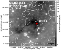
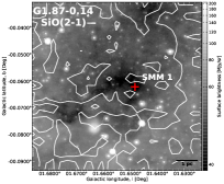
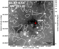
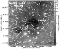
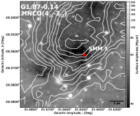
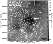
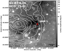
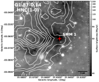
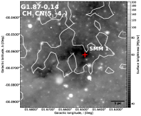
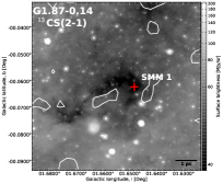
Figure 3: Contour maps of integrated intensity of the MALT90 lines detected towards G1.87–SMM 1. In each panel, the contours are overlaid on the arcsinh-scaled Spitzer 8-$\mu$m image (cf. Fig. 1). The contour levels start at $3\sigma$ for H¹³CO⁺, SiO, HN¹³C, C₂H, CH₃CN, and ¹³CS. For HNCO$(4_{0,\,4}-3_{0,\,3})$, HCN, HCO⁺, HNC, HC₃N, and N₂H⁺, the contours start at $26\sigma$, $23\sigma$, $20\sigma$, $30\sigma$, $6\sigma$, and $15\sigma$, respectively. In all cases, the contours go in steps of $3\sigma$. The average $1\sigma$ value in $T_{\rm MB}$ units is $\sim 0.69$ K km s^-1. The red plus sign marks the LABOCA 870-$\mu$m peak position of the clump. A scale bar indicating the 1 pc projected length is indicated. The line emission is extended in many cases, and the HCN, HCO⁺, and HNC emissions are well correlated with each other. The N₂H⁺ emission also shows some resemblance to these species. The spatial distributions of HNCO and HC₃N appear to be similar to each other, while weak CH₃CN emission traces reasonably well the 8-$\mu$m absorption feature.

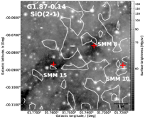
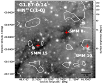
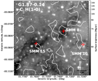
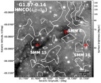
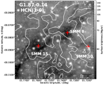
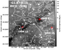
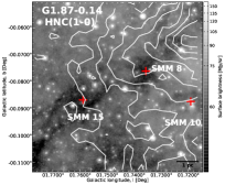
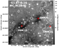
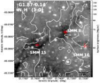
Figure 4: Similar to Fig. 3 but towards G1.87–SMM 8, 10, 15. The contour levels start at $3\sigma$ for SiO, HN¹³C, C₂H, and HC₃N. For HNCO$(4_{0,\,4}-3_{0,\,3})$, HCN, HCO⁺, HNC, and N₂H⁺, the contours start at $9\sigma$, $16\sigma$, $15\sigma$, $12\sigma$, and $5\sigma$, respectively. In all cases, the contours go in steps of $3\sigma$. The average $1\sigma$ value in $T_{\rm MB}$ units is $\sim 0.70$ K km s^-1. The LABOCA 870-$\mu$m peak positions of the clumps are marked by red plus signs. A scale bar indicating the 1 pc projected length is indicated. The spatial distributions of the HCN, HCO⁺, and HNC emissions appear to be quite similar. Those of HNCO and N₂H⁺ show some similarities also.

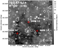
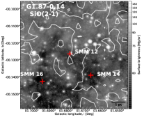
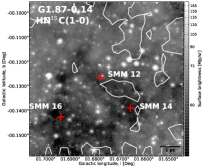
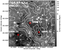
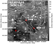
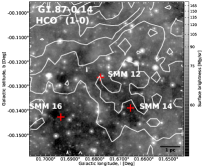
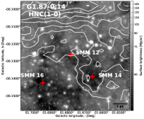
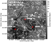
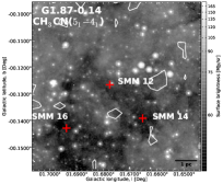
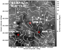
Figure 5: Similar to Fig. 3 but towards G1.87–SMM 12, 14, 16. The contour levels start at $3\sigma$ for H¹³CO⁺, HN¹³C, C₂H, HC₃N, and CH₃CN. For SiO, HNCO$(4_{0,\,4}-3_{0,\,3})$, HCN, HCO⁺, HNC, and N₂H⁺, the contours start at $5\sigma$, $15\sigma$, $19\sigma$, $10\sigma$, $15\sigma$, and $6\sigma$, respectively. In all cases, the contours go in steps of $3\sigma$. The average $1\sigma$ value in $T_{\rm MB}$ units is $\sim 0.63$ K km s^-1. The LABOCA 870-$\mu$m peak positions of the clumps are marked by red plus signs. A scale bar indicating the 1 pc projected length is indicated. The emissions of HNCO, HCN, HCO⁺, HNC, HC₃N, and N₂H⁺ are extended in a similar fashion, but HNCO clearly shows the strongest.

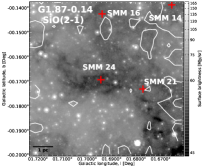
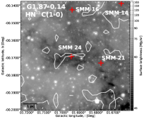
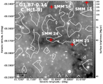
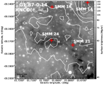
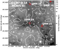
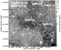
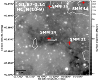
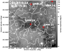
Figure 6: Similar to Fig. 3 but towards G1.87–SMM 14, 16, 17, 21, 24. The contour levels start at $3\sigma$ for SiO, HN¹³C, C₂H, and HC₃N. For HNCO$(4_{0,\,4}-3_{0,\,3})$, HCN, HCO⁺, HNC, and N₂H⁺, the contours start at $8\sigma$, $8\sigma$, $5\sigma$, $5\sigma$, and $5\sigma$, respectively. In all cases, the contours go in steps of $3\sigma$. The average $1\sigma$ value in $T_{\rm MB}$ units is $\sim 0.78$ K km s^-1. The LABOCA 870-$\mu$m peak positions of the clumps are marked by red plus signs. The 870-$\mu$m peak of SMM 17 (west of SMM 21) lies just outside the MALT90 map (cf. Fig. 1, middle left panel). A scale bar indicating the 1 pc projected length is indicated. The HCN and HNC emissions show some morphological similarities.

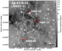
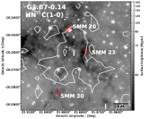
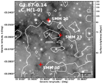
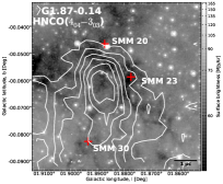
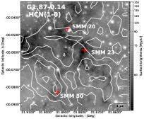
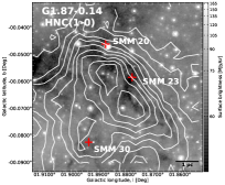
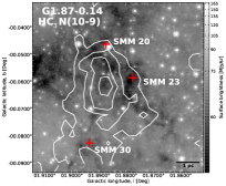
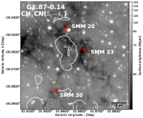
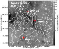
Figure 7: Similar to Fig. 3 but towards G1.87–SMM 20, 23, 30. The contour levels start at $3\sigma$ for HN¹³C, C₂H, and CH₃CN, and $5\sigma$ for SiO, HNCO$(4_{0,\,4}-3_{0,\,3})$, HCN, HCO⁺, HNC, HC₃N, and N₂H⁺. In all cases, the contours go in steps of $3\sigma$. The average $1\sigma$ value in $T_{\rm MB}$ units is $\sim 0.63$ K km s^-1. The LABOCA 870-$\mu$m peak positions of the clumps are marked by red plus signs. A scale bar indicating the 1 pc projected length is indicated. Good correlations are seen between the peak emissions of SiO, HNCO, HC₃N, CH₃CN, and N₂H⁺. The HNC emission also shows it maxima in between the submm peaks.

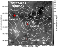
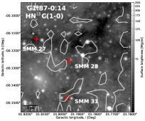
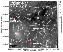
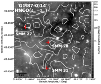
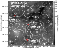
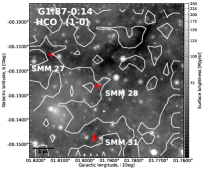
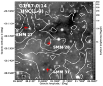
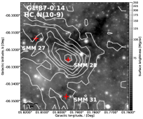
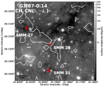
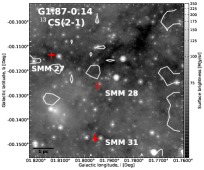
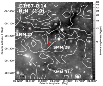
Figure 8: Similar to Fig. 3 but towards G1.87–SMM 27, 28, 31. The contour levels start at $3\sigma$ for SiO, HN¹³C, C₂H, CH₃CN, and ¹³CS. For, HNCO$(4_{0,\,4}-3_{0,\,3})$, HNC, HCN, HCO⁺, HC₃N, and N₂H⁺, the contours start at $9\sigma$, $7\sigma$, $7\sigma$, $4\sigma$, $4\sigma$, and $5\sigma$, respectively. In all cases, the contours go in steps of $3\sigma$. The average $1\sigma$ value in $T_{\rm MB}$ units is $\sim 0.63$ K km s^-1. The LABOCA 870-$\mu$m peak positions are marked by red plus signs. A scale bar indicating the 1 pc projected length is indicated. The SiO and HC₃N emission morphologies resemble each other. Also HNC and N₂H⁺ share some common features (e.g., peak close to SMM 28).

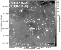
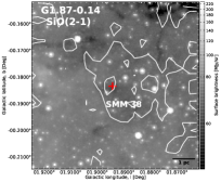
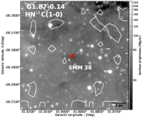
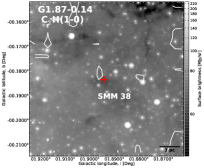
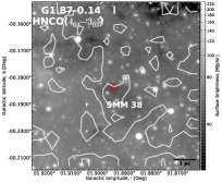
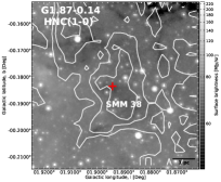
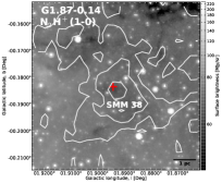
Figure 9: Similar to Fig. 3 but towards G1.87–SMM 38. The contour levels start at $3\sigma$ for H¹³CO⁺, SiO, HN¹³C, C₂H, HNCO$(4_{0,\,4}-3_{0,\,3})$, HC₃N, and N₂H⁺. For HNC, the contours start at $5\sigma$. In all cases, the contours go in steps of $3\sigma$. The average $1\sigma$ value in $T_{\rm MB}$ units is $\sim 0.77$ K km s^-1. The clump’s LABOCA 870-$\mu$m peak position is marked by a red plus sign. A scale bar indicating the 1 pc projected length is indicated. Note that the SiO, HNC, HC₃N, and N₂H⁺ emissions peak towards the submm maximum. HNC and N₂H⁺ also show otherwise comparable spatial distributions.

Appendix C Spectra

The Hanning-smoothed spectra of the detected spectral lines are presented in Figs. 17–49. In each panel, the fit to the line is superimposed as a green line.

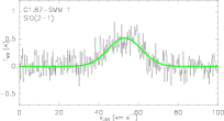
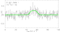
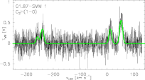
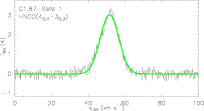
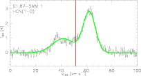
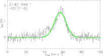
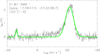
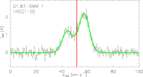
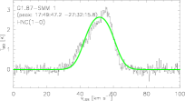
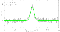
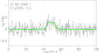
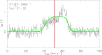
Figure 17: Hanning-smoothed spectra towards G1.87–SMM 1. The single Gaussian and hf structure fits are shown with green lines. The red vertical line plotted on double-peaked profiles indicates the radial velocity of the optically thin HC₃N line. The velocity range is wider in the C₂H and HCO⁺ (line emission peak) spectra than in the other panels to show all the detected lines (additional velocity component in the latter case).

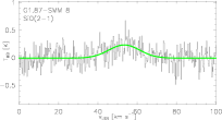
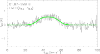
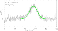
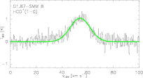
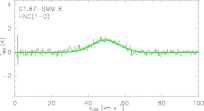
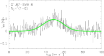
Figure 18: Same as Fig. 17 but towards G1.87–SMM 8.

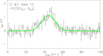
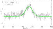
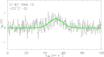
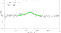
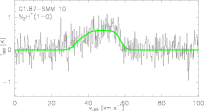
Figure 19: Same as Fig. 17 but towards G1.87–SMM 10.

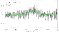
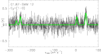
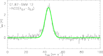
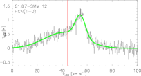
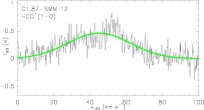
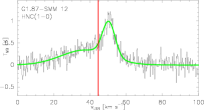
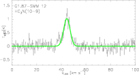
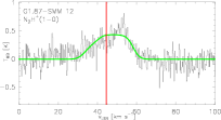
Figure 20: Same as Fig. 17 but towards G1.87–SMM 12. Note that the velocity range for the SiO and C₂H spectra is wider for illustrative purposes. The red vertical line marks the radial velocity of the optically thin HC₃N line.

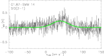
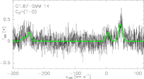
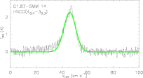
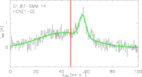
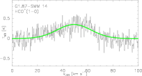
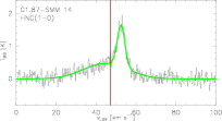
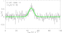
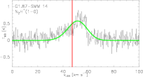
Figure 21: Same as Fig. 17 but towards G1.87–SMM 14. Note that the velocity range for the SiO and C₂H spectra is wider for illustrative purposes. The red vertical line marks the radial velocity of the optically thin HC₃N line.

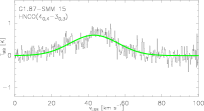
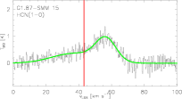
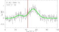
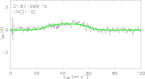
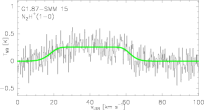
Figure 22: Same as Fig. 17 but towards G1.87–SMM 15. The red vertical line indicates the radial velocity of the optically thin HNCO line.

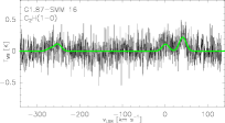
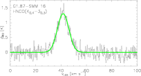
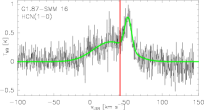
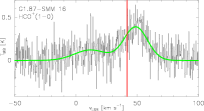
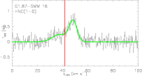
Figure 23: Same as Fig. 17 but towards G1.87–SMM 16. In some of the spectra, the velocity range shown is wider for illustrative purposes. The red vertical line mark the velocity of the HNCO line.

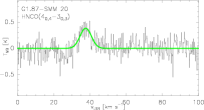
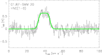
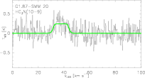
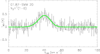
Figure 24: Same as Fig. 17 but towards G1.87–SMM 20.

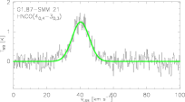
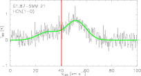
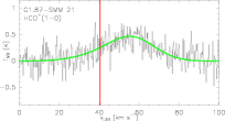
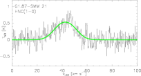
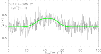
Figure 25: Same as Fig. 17 but towards G1.87–SMM 21. The red vertical line indicates the radial velocity of the HNCO line.

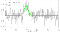
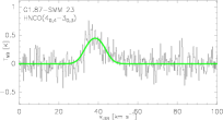
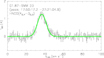
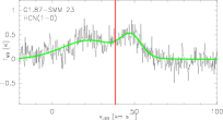
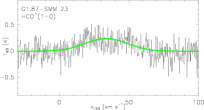
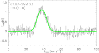
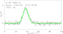
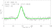
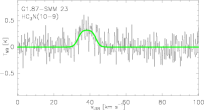
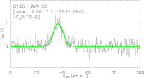
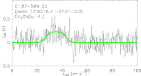
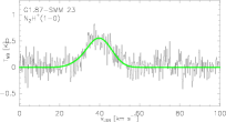
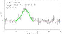
Figure 26: Same as Fig. 17 but towards G1.87–SMM 23. Note that the velocity range for the HCN and HCO⁺ spectra is wider for illustrative purposes. The red vertical line indicates the radial velocity of the optically thin HC₃N line.

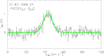
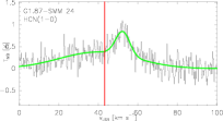
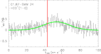
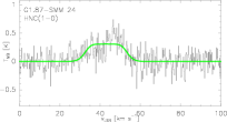
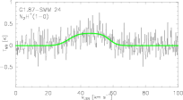
Figure 27: Same as Fig. 17 but towards G1.87–SMM 24. The red vertical line indicates the radial velocity of the HNCO line.

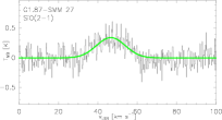
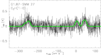
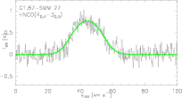
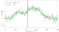
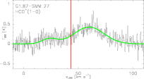
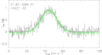
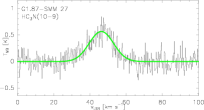
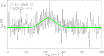
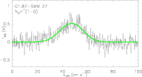
Figure 28: Same as Fig. 17 but towards G1.87–SMM 27. The velocity range shown is wider for the C₂H and HCO⁺ spectra. The red vertical line indicates the radial velocity of the optically thin HNCO line.

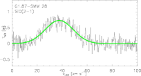
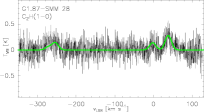
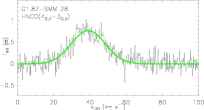
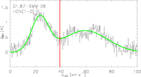
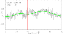
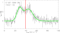
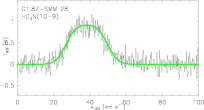
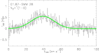
Figure 29: Same as Fig. 17 but towards G1.87–SMM 28. The velocity range shown is wider for the C₂H spectrum. The red vertical line indicates the radial velocity of the optically thin HNCO line.

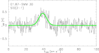
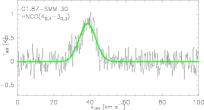
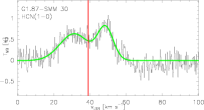
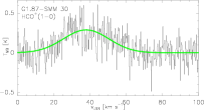
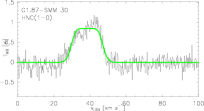
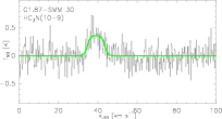
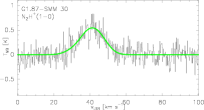
Figure 30: Same as Fig. 17 but towards G1.87–SMM 30. The red vertical line indicates the radial velocity of the optically thin HC₃N line.

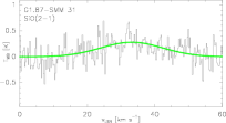
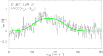
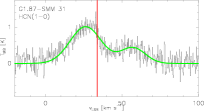
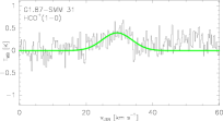
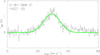
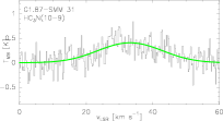
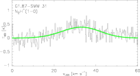
Figure 31: Same as Fig. 17 but towards G1.87–SMM 31. The velocity range is wider for the HCN spectrum. The red vertical line indicates the radial velocity of the optically thin HNCO line.

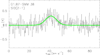
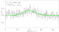
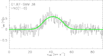
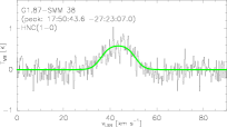
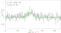
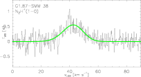
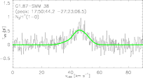
Figure 32: Same as Fig. 17 but towards G1.87–SMM 38.

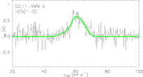
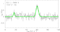
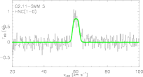
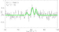
Figure 33: Same as Fig. 17 but towards G2.11–SMM 5. A wider velocity range for the HCO⁺ spectrum is shown due to the additional velocity component.

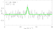
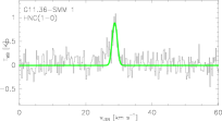
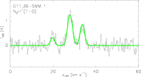
Figure 34: Same as Fig. 17 but towards G11.36–SMM 1.

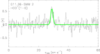
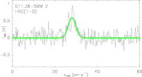
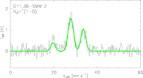
Figure 35: Same as Fig. 17 but towards G11.36–SMM 2.

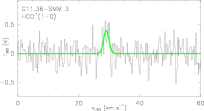
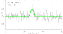
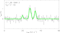
Figure 36: Same as Fig. 17 but towards G11.36–SMM 3.

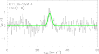
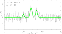
Figure 37: Same as Fig. 17 but towards G11.36–SMM 4.

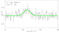
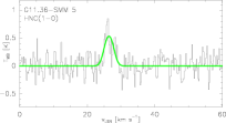
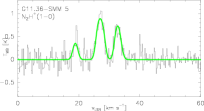
Figure 38: Same as Fig. 17 but towards G11.36–SMM 5.

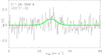
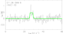
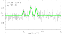
Figure 39: Same as Fig. 17 but towards G11.36–SMM 6.

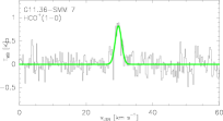
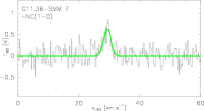
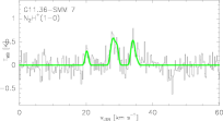
Figure 40: Same as Fig. 17 but towards G11.36–SMM 7.

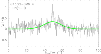
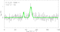
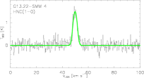
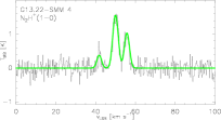
Figure 41: Same as Fig. 17 but towards G13.22–SMM 4. There is an additional velocity component in the HCO⁺ spectrum.

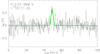
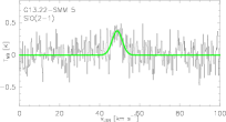
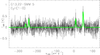
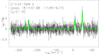
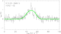
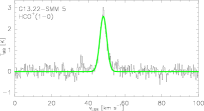
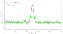
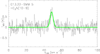
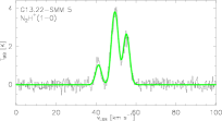
Figure 42: Same as Fig. 17 but towards G13.22–SMM 5. The velocity range is wider for the two C₂H spectra.

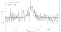
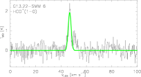
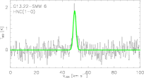
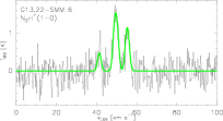
Figure 43: Same as Fig. 17 but towards G13.22–SMM 6.

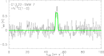
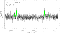
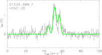
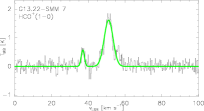
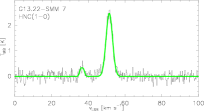
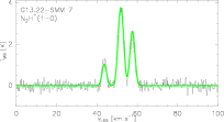
Figure 44: Same as Fig. 17 but towards G13.22–SMM 7. The C₂H spectrum has a wider velocity range. Two velocity components are seen in the HCO⁺ and HNC spectra.

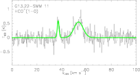
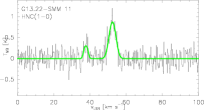
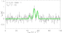
Figure 45: Same as Fig. 17 but towards G13.22–SMM 11. Two velocity components are seen in the HCO⁺ and HNC spectra.

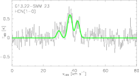
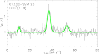
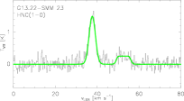
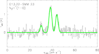
Figure 46: Same as Fig. 17 but towards G13.22–SMM 23. Three velocity components are seen in the HCO⁺ spectrum, while two are visible in the HNC spectrum.

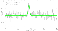
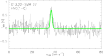
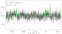
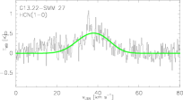
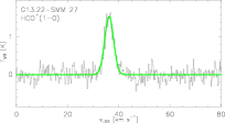
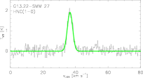
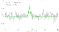
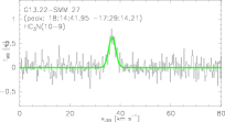
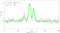
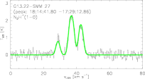
Figure 47: Same as Fig. 17 but towards G13.22–SMM 27. The velocity range in the C₂H spectrum is wider.

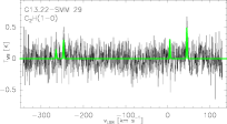
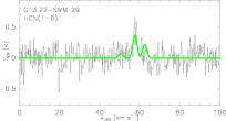
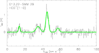
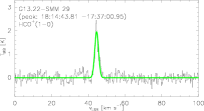
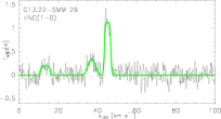
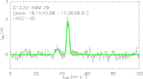
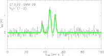
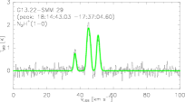
Figure 48: Same as Fig. 17 but towards G13.22–SMM 29. The velocity range in the C₂H spectrum is wider. Four velocity components are seen in the HCO⁺ spectrum, three in the HNC spectrum towards the LABOCA peak, and two in the HNC spectrum towards the line emission peak.

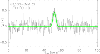
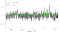
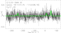
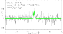
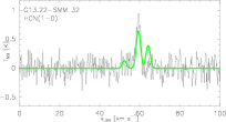
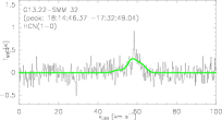
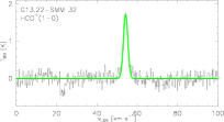
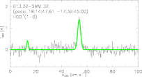
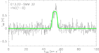
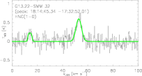
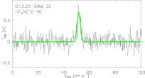
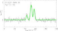
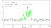
Figure 49: Same as Fig. 17 but towards G13.22–SMM 32. The velocity range for the C₂H spectra is wider. Two velocity components are detected in the HCO⁺ and HNC spectra towards the line emission peaks.

Table 6: Spectral-line parameters, beam-averaged molecular column densities, and fractional abundances with respect to H₂.

Source	Transition	${\rm v}_{\rm LSR}$	$\Delta{\rm v}$	$T_{\rm MB}$	$\int T_{\rm MB}{\rm dv}$	$\tau$	$T_{\rm ex}$	$N$	$x$
		[km s-1]	[km s-1]	[K]	[K km s-1]		[K]	[cm-2]	[$10^{-10}$]
G1.87-0.14
SMM 1	SiO$(2-1)$	$53.1\pm 0.5$	$19.56\pm 1.02$	$0.52\pm 0.24$	$10.84\pm 0.50$	$0.17\pm 0.01$	$=E_{\rm u}=6.25$	$2.5\pm 0.1(13)$	$2.6\pm 0.3$
	HN13C$(1-0)$	$54.1\pm 0.6$	$9.29\pm 2.67$	$0.26\pm 0.21$(G)	$3.83\pm 0.40$(G)	$0.29\pm 0.03$	$5.2\pm 0.1$(A)	$9.6\pm 1.0(12)$	$1.0\pm 0.1$
	C2H$(1-0)$	$52.0\pm 0.3$	$11.30\pm 0.71$	$0.57\pm 0.23$(S)	$8.63\pm 0.51$(S)	$2.38\pm 1.00$	$3.8\pm 0.5$	$1.2\pm 0.5(15)$	$125.4\pm 53.7$
	HNCO$(4_{0,\,4}-3_{0,\,3})$	$51.6\pm 0.1$	$11.70\pm 0.14$	$3.04\pm 0.25$(G)	$38.68\pm 0.42$(G)	$2.86\pm 0.39$	$=2E_{\rm u}/3=7.03$	$7.9\pm 1.1(14)$	$82.5\pm 14.1$
	HCN$(1-0)$	$41.9\pm 0.4$(B)/	$20.10\pm 0.89$(B)/	$0.97\pm 0.37$(B)/	$20.78\pm 0.80$(B)/	…	…	…	…
		$62.3\pm 0.1$(R)	$11.55\pm 0.25$(R)	$2.77\pm 0.37$(R)	$34.09\pm 0.72$(R)	…	…	…	…
	HCO${}^{+}(1-0)$	$56.8\pm 0.2$	$14.76\pm 0.43$	$1.58\pm 0.29$	$24.84\pm 0.53$	$1.67\pm 0.74$	$4.9\pm 0.2$(A)	$6.3\pm 2.8(13)$	$6.6\pm 3.0$
	HCO${}^{+}(1-0)$	$53.8\pm 0.1$	$16.13\pm 0.28$	$2.24\pm 0.31$	$38.38\pm 0.53$	…	$4.9\pm 0.2$(A)	$3.5\pm 0.1(13)$	$3.7\pm 0.4$
		$-41.5\pm 0.6$	$3.37\pm 1.05$	$0.52\pm 0.22$	$1.87\pm 0.60$	$0.31\pm 0.05$	$4.9\pm 0.2$(A)	$2.3\pm 0.7(12)$	$0.7\pm 0.2$
	HNC$(1-0)$	$52.0\pm 0.1$	$10.60\pm 0.37$	…	…	$17.20\pm 3.60$	$4.5\pm 0.1$(A)	$5.3\pm 1.1(14)$	$55.4\pm 12.7$
		$44.3\pm 0.2$(B)/	$9.47\pm 0.53$(B)/	$1.21\pm 0.24$(B)/	$12.24\pm 0.62$(B)/	…	…	…	…
		$57.2\pm 0.1$(R)	$9.86\pm 0.29$(R)	$2.19\pm 0.24$(R)	$22.95\pm 0.62$(R)	…	…	…	…
	HNC$(1-0)$	$51.8\pm 0.1$	$15.40\pm 0.15$	…	…	$1.43\pm 0.01$	$4.5\pm 0.1$(A)	$6.4\pm 0.1(13)$	$14.7\pm 1.5$
		$48.6\pm 0.4$(B)/	$17.96\pm 0.48$(B)/	$2.01\pm 0.20$(B)/	$38.37\pm 2.03$(B)/	…	…	…	…
		$56.5\pm 0.1$(R)	$7.93\pm 0.46$(R)	$1.72\pm 0.20$(R)	$14.53\pm 1.77$(R)	…	…	…	…
	HC3N$(10-9)$	$51.6\pm 0.1$	$7.74\pm 0.25$	$1.66\pm 0.24$(G)	$13.92\pm 0.35$(G)	$0.23\pm 0.01$	$=E_{\rm u}=24.01$	$5.8\pm 0.1(13)$	$6.1\pm 0.6$
	CH3CN$(5_{1}-4_{1})$	$48.5\pm 0.4$	$5.85\pm 0.69$	$0.32\pm 0.23$(G)	$3.07\pm 0.31$(G)	$0.03\pm 0.01$	$=2E_{\rm u}/3=13.59$	$4.2\pm 0.4(11)$	$0.04\pm 0.01$
	N2H${}^{+}(1-0)$	$53.5\pm 0.3$	$8.85\pm 0.53$	…	…	$10.70\pm 1.84$	$7.2\pm 0.2$(A)	$5.4\pm 1.0(14)$	$56.4\pm 11.8$
		$46.4\pm 0.1$(B)/	$13.98\pm 0.11$(B)/	$0.58\pm 0.25$(B)/	$8.60\pm 0.05$(B)/	…	…	…	…
		$60.5\pm 0.1$(R)	$9.71\pm 0.11$(R)	$1.14\pm 0.25$(R)	$11.80\pm 0.05$(R)	…	…	…	…
SMM 8	SiO$(2-1)$	$53.4\pm 1.0$	$18.54\pm 2.48$	$0.24\pm 0.22$	$4.71\pm 0.53$	$0.08\pm 0.01$	$=E_{\rm u}=6.25$	$1.1\pm 0.1(13)$	$3.5\pm 0.5$
	HNCO$(4_{0,\,4}-3_{0,\,3})$	$45.5\pm 0.5$	$17.00\pm 1.52$	$0.63\pm 0.23$(G)	$14.70\pm 0.61$(G)	$0.34\pm 0.02$	$=2E_{\rm u}/3=7.03$	$6.1\pm 0.3(14)$	$193.2\pm 21.7$
	HCN$(1-0)$	$55.0\pm 0.1$	$13.50\pm 0.38$	$1.35\pm 0.26$(G)	$25.19\pm 0.57$(G)	$0.89\pm 0.10$	$6.5\pm 0.8$	$1.4\pm 0.2(14)$	$44.3\pm 7.8$
	HCO${}^{+}(1-0)$	$54.1\pm 0.3$	$18.17\pm 0.71$	$1.06\pm 0.26$	$20.45\pm 0.63$	$0.79\pm 0.19$	$4.9\pm 0.2$(A)	$3.6\pm 0.9(13)$	$11.4\pm 3.1$
	HNC$(1-0)$	$49.4\pm 0.3$	$17.90\pm 0.82$	$1.05\pm 0.23$(G)	$20.18\pm 0.79$(G)	$2.00\pm 0.55$	$4.5\pm 0.1$(A)	$1.0\pm 0.3(14)$	$31.7\pm 10.0$
	N2H${}^{+}(1-0)$	$46.6\pm 0.6$	$20.10\pm 1.69$	$0.47\pm 0.23$(G)	$12.90\pm 0.62$(G)	$1.26\pm 0.39$	$4.6\pm 1.0$	$7.2\pm 3.9(13)$	$22.8\pm 12.6$
SMM 10	HNCO$(4_{0,\,4}-3_{0,\,3})$	$44.3\pm 0.3$	$17.00\pm 0.85$	$1.14\pm 0.38$(G)	$20.88\pm 0.85$	$0.67\pm 0.07$	$=2E_{\rm u}/3=7.03$	$2.7\pm 0.3(14)$	$188.5\pm 29.3$
	HCN$(1-0)$	$51.7\pm 0.3$	$14.30\pm 0.90$	$1.38\pm 0.41$	$24.74\pm 0.91$	$1.87\pm 0.94$	$5.1\pm 0.5$(A)	$2.2\pm 1.1(14)$	$153.6\pm 78.6$
	HCO${}^{+}(1-0)$	$51.8\pm 0.6$	$17.33\pm 1.74$	$0.61\pm 0.40$	$11.35\pm 0.89$	$0.38\pm 0.10$	$4.9\pm 0.2$(A)	$1.4\pm 0.1(13)$	$9.8\pm 1.3$
	HNC$(1-0)$	$46.1\pm 0.5$	$18.90\pm 1.40$	$1.09\pm 0.39$(G)	$22.21\pm 1.21$(G)	$2.15\pm 0.98$	$4.5\pm 0.1$(A)	$1.2\pm 0.5(14)$	$83.8\pm 36.1$
	N2H${}^{+}(1-0)$	$45.7\pm 0.6$	$8.33\pm 1.45$	$0.64\pm 0.38$(G)	$14.68\pm 0.91$(G)	$8.08\pm 3.16$	$3.6\pm 0.5$	$1.4\pm 2.6(14)$	$97.7\pm 181.8$
SMM 12	SiO$(2-1)$	$34.0\pm 1.5$	$49.27\pm 3.32$	$0.23\pm 0.20$	$11.95\pm 0.72$	$0.07\pm 0.01$	$=E_{\rm u}=6.25$	$2.8\pm 0.2(13)$	$7.8\pm 1.0$
	C2H$(1-0)$	$44.6\pm 0.2$	$5.67\pm 0.61$	$0.40\pm 0.21$(S)	$2.86\pm 0.27$(S)	$4.07\pm 2.14$	$3.3\pm 0.3$	$8.8\pm 4.7(14)$	$244.0\pm 132.6$
	HNCO$(4_{0,\,4}-3_{0,\,3})$	$44.2\pm 0.1$	$8.41\pm 0.15$	$2.64\pm 0.27$(G)	$24.13\pm 0.34$(G)	$2.17\pm 0.26$	$=2E_{\rm u}/3=7.03$	$4.3\pm 0.5(14)$	$119.2\pm 18.3$
	HCN$(1-0)$	$47.4\pm 0.4$	$30.40\pm 0.87$	…	…	…	…	…	…
		$41.5\pm 0.9$(B)/	$37.51\pm 1.45$(B)/	$0.56\pm 0.20$(B)/	$22.48\pm 1.03$(B)/	…	…	…	…
		$54.6\pm 0.2$(R)	$9.51\pm 0.65$(R)	$0.79\pm 0.20$(R)	$8.00\pm 0.70$(R)	…	…	…	…
	HCO${}^{+}(1-0)$	$44.9\pm 0.7$	$41.65\pm 1.58$	$0.46\pm 0.20$	$20.44\pm 0.65$	$0.27\pm 0.04$	$4.9\pm 0.2$(A)	$2.5\pm 0.1(13)$	$6.9\pm 0.7$
	HNC$(1-0)$	$46.9\pm 0.4$	$22.70\pm 1.11$	…	…	$1.07\pm 0.22$	$4.5\pm 0.1$(A)	$7.1\pm 1.5(13)$	$19.7\pm 4.6$
		$41.1\pm 0.9$(B)/	$31.45\pm 1.63$(B)/	$0.41\pm 0.13$(B)/	$13.77\pm 0.77$(B)/	…	…	…	…
		$50.8\pm 0.2$(R)	$6.37\pm 0.54$(R)	$0.72\pm 0.13$(R)	$4.86\pm 0.47$(R)	…	…	…	…
	HC3N$(10-9)$	$44.5\pm 0.1$	$6.05\pm 0.28$	$1.02\pm 0.21$(G)	$6.70\pm 0.28$	$0.14\pm 0.01$	$=E_{\rm u}=24.01$	$2.8\pm 0.1(13)$	$7.8\pm 0.8$
	N2H${}^{+}(1-0)$	$46.3\pm 0.5$	$8.84\pm 1.21$	$0.47\pm 0.20$(G)	$10.03\pm 0.50$(G)	$6.54\pm 2.19$	$3.4\pm 0.3$	$1.1\pm 2.0(14)$	$30.5\pm 55.5$
SMM 14	SiO$(2-1)$	$38.7\pm 2.0$	$50.97\pm 6.00$	$0.22\pm 0.22$	$12.07\pm 0.95$	$0.07\pm 0.01$	$=E_{\rm u}=6.25$	$2.8\pm 0.2(13)$	$5.7\pm 0.7$
	C2H$(1-0)$	$45.7\pm 0.5$	$14.30\pm 0.70$	$0.39\pm 0.21$(S)	$6.18\pm 0.55$(S)	$0.94\pm 0.20$	$4.1\pm 0.1$(A)	$6.5\pm 1.3(14)$	$132.8\pm 29.7$
	HNCO$(4_{0,\,4}-3_{0,\,3})$	$46.1\pm 0.1$	$10.60\pm 0.20$	$2.30\pm 0.26$(G)	$26.47\pm 0.41$(G)	$1.72\pm 0.17$	$=2E_{\rm u}/3=7.03$	$4.3\pm 0.4(14)$	$87.9\pm 12.0$
	HCN$(1-0)$	$46.1\pm 0.1$	$41.30\pm 0.38$	…	…	…	…	…	…
		$39.3\pm 0.2$(B)/	$45.85\pm 1.6$(B)/	$0.59\pm 0.22$(B)/	$28.99\pm 0.98$(B)/	…	…	…	…
		$56.7\pm 0.2$(R)	$7.41\pm 0.55$(R)	$0.89\pm 0.22$(R)	$6.98\pm 0.43$(R)	…	…	…	…
	HCO${}^{+}(1-0)$	$49.1\pm 0.8$	$32.09\pm 1.72$	$0.35\pm 0.21$	$11.94\pm 0.58$	$0.20\pm 0.03$	$4.9\pm 0.2$(A)	$1.5\pm 0.1(13)$	$3.1\pm 0.4$
	HNC$(1-0)$	$51.4\pm 0.2$	$10.80\pm 0.61$	…	…	$2.78\pm 0.91$	$4.5\pm 0.1$(A)	$8.8\pm 2.9(13)$	$18.0\pm 6.2$
		$44.8\pm 0.7$(B)/	$26.50\pm 1.32$(B)/	$0.47\pm 0.14$(B)/	$13.33\pm 0.63$(B)/	…	…	…	…
		$52.5\pm 0.1$(R)	$4.61\pm 0.25$(R)	$1.27\pm 0.14$(R)	$6.21\pm 0.36$(R)	…	…	…	…
	HC3N$(10-9)$	$47.2\pm 0.3$	$10.40\pm 0.62$	$0.56\pm 0.19$(G)	$6.28\pm 0.35$(G)	$0.07\pm 0.01$	$=E_{\rm u}=24.01$	$2.6\pm 0.1(13)$	$5.3\pm 0.6$
	N2H${}^{+}(1-0)$	$49.8\pm 0.5$	$10.70\pm 2.40$	$0.56\pm 0.22$(G)	$11.41\pm 0.51$	$1.85\pm 0.70$	$4.4\pm 0.8$	$5.3\pm 3.6(13)$	$10.8\pm 5.4$
SMM 15	HNCO$(4_{0,\,4}-3_{0,\,3})$	$43.2\pm 0.5$	$30.40\pm 1.39$	$0.63\pm 0.24$(G)	$20.76\pm 0.80$(G)	$0.34\pm 0.02$	$=2E_{\rm u}/3=7.03$	$1.1\pm 0.1(14)$	$48.6\pm 6.6$
	HCN$(1-0)$	$51.5\pm 0.5$	$23.40\pm 1.24$	…	…	…	…	…	…
		$38.5\pm 0.1$(B)/	$37.71\pm 0.11$(B)/	$0.23\pm 0.27$(B)/	$9.41\pm 0.06$(B)/	…	…	…	…
		$54.5\pm 0.1$(R)	$18.49\pm 0.11$(R)	$0.79\pm 0.27$(R)	$15.64\pm 0.06$(R)	…	…	…	…
	HCO${}^{+}(1-0)$	$27.3\pm 1.2$(B)/	$14.04\pm 2.38$(B)/	$0.24\pm 0.18$(B)/	$3.66\pm 0.56$(B)/	…	…	…	…
		$53.7\pm 0.4$(R)	$19.26\pm 1.03$(R)	$0.75\pm 0.18$(R)	$15.43\pm 0.66$(R)	…	…	…	…
	HNC$(1-0)$	$43.4\pm 0.8$	$21.20\pm 2.81$	$0.59\pm 0.23$(G)	$18.32\pm 1.00$(G)	$3.46\pm 2.24$	$3.5\pm 0.3$	$1.5\pm 1.0(14)$	$66.2\pm 44.7$
	N2H${}^{+}(1-0)$	$39.4\pm 0.7$	$17.00\pm 0.70$	$0.31\pm 0.23$(G)	$12.08\pm 0.63$(G)	$0.30\pm 0.02$	$7.2\pm 0.2$(A)	$1.6\pm 0.1(13)$	$7.1\pm 0.8$
SMM 16	C2H$(1-0)$	$41.5\pm 0.9$	$18.90\pm 2.41$	$0.24\pm 0.21$(S)	$4.31\pm 0.48$(S)	$0.53\pm 0.11$	$4.1\pm 0.1$(A)	$1.7\pm 0.2(14)$	$50.8\pm 7.9$
	HNCO$(4_{0,\,4}-3_{0,\,3})$	$41.7\pm 0.1$	$10.80\pm 0.30$	$1.33\pm 0.21$(G)	$15.51\pm 0.36$(G)	$0.81\pm 0.05$	$=2E_{\rm u}/3=7.03$	$2.1\pm 0.1(14)$	$62.7\pm 7.0$
	HCN$(1-0)$	$36.6\pm 1.1$	$38.30\pm 0.54$	…	…	$3.66\pm 0.33$	$5.1\pm 0.5$(A)	$1.2\pm 0.1(15)$	$358.4\pm 46.9$
		$32.5\pm 1.5$(B)/	$59.84\pm 2.58$(B)/	$0.36\pm 0.21$(B)/	$23.09\pm 1.07$(B)/	…	…	…	…
		$52.8\pm 0.3$(R)	$10.48\pm 0.98$(R)	$0.54\pm 0.21$(R)	$6.03\pm 0.59$(R)	…	…	…	…
	HCO${}^{+}(1-0)$	$13.6\pm 3.5$(B)/	$32.86\pm 7.73$(B)/	$0.10\pm 0.14$(B)/	$3.40\pm 0.71$(B)/	…	…	…	…
		$48.9\pm 0.7$(R)	$19.18\pm 1.61$(R)	$0.36\pm 0.14$(R)	$7.39\pm 0.61$(R)	…	…	…	…
	HNC$(1-0)$	$47.0\pm 0.3$	$11.30\pm 1.02$	…	…	…	…	…	…
		$37.6\pm 2.8$(B)/	$13.79\pm 3.82$(B)/	$0.24\pm 0.21$(B)/	$3.52\pm 1.20$(B)/	…	…	…	…
		$48.3\pm 0.5$(R)	$7.42\pm 1.05$(R)	$0.68\pm 0.21$(R)	$5.34\pm 1.24$(R)	…	…	…	…
SMM 20	HNCO$(4_{0,\,4}-3_{0,\,3})$	$37.4\pm 0.2$	$2.90\pm 0.20$	$0.38\pm 0.19$(G)	$3.03\pm 0.31$(G)	$0.20\pm 0.01$	$=2E_{\rm u}/3=7.03$	$1.7\pm 0.2(13)$	$6.1\pm 1.0$
	HNC$(1-0)$	$39.2\pm 0.2$	$7.16\pm 0.54$	$0.71\pm 0.19$(G)	$8.60\pm 0.33$(G)	$7.30\pm 2.71$	$3.6\pm 0.2$	$1.1\pm 0.4(14)$	$39.4\pm 14.9$
	HC3N$(10-9)$	$37.4\pm 0.6$	$8.25\pm 1.36$	$0.30\pm 0.25$(G)	$3.13\pm 0.38$(G)	$1.46\pm 0.68$	$3.6\pm 0.7$	$4.9\pm 2.4(14)$	$175.5\pm 87.8$
	N2H${}^{+}(1-0)$	$38.7\pm 0.4$	$10.00\pm 2.47$	$0.45\pm 0.21$(G)	$7.62\pm 0.40$(G)	$0.45\pm 0.03$	$7.2\pm 0.2$(A)	$9.9\pm 0.5(12)$	$3.5\pm 0.4$
SMM 21	HNCO$(4_{0,\,4}-3_{0,\,3})$	$40.4\pm 0.2$	$11.80\pm 0.41$	$1.34\pm 0.26$(G)	$17.12\pm 0.48$	$0.82\pm 0.06$	$=2E_{\rm u}/3=7.03$	$2.3\pm 0.2(14)$	$116.5\pm 15.7$
	HCN$(1-0)$	$46.9\pm 0.6$	$28.90\pm 1.46$	…	…	…	…	…	…
		$30.1\pm 2.2$(B)/	$19.97\pm 4.69$(B)/	$0.32\pm 0.27$(B)/	$6.79\pm 1.71$(B)/	…	…	…	…
		$51.9\pm 0.9$(R)	$18.30\pm 1.84$(R)	$0.75\pm 0.27$(R)	$14.60\pm 1.71$(R)	…	…	…	…
	HCO${}^{+}(1-0)$	$40.3\pm 2.3$(B)/	$6.95\pm 3.76$(B)/	$0.06\pm 0.27$(B)/	$0.45\pm 0.50$(B)/	…	…	…	…
		$55.0\pm 0.8$(R)	$30.89\pm 2.76$(R)	$0.45\pm 0.27$(R)	$14.72\pm 1.16$(R)	…	…	…	…
	HNC$(1-0)$	$42.6\pm 0.5$	$17.30\pm 0.86$	$0.54\pm 0.25$(G)	$11.04\pm 0.58$(G)	$0.76\pm 0.15$	$4.5\pm 0.1$(A)	$3.8\pm 0.8(13)$	$19.2\pm 4.5$
	N2H${}^{+}(1-0)$	$41.8\pm 0.7$	$16.10\pm 2.24$	$0.39\pm 0.26$(G)	$9.70\pm 0.63$(G)	$2.24\pm 0.71$	$3.8\pm 0.7$	$7.8\pm 1.3(13)$	$39.5\pm 7.7$
SMM 23	SiO$(2-1)$	$39.2\pm 0.5$	$9.65\pm 1.08$	$0.34\pm 0.21$	$3.50\pm 0.33$	$0.11\pm 0.01$	$=E_{\rm u}=6.25$	$8.2\pm 0.8(12)$	$1.6\pm 0.2$
	HNCO$(4_{0,\,4}-3_{0,\,3})$	$38.4\pm 0.5$	$9.77\pm 2.28$	$0.46\pm 0.21$(G)	$5.42\pm 0.38$(G)	$0.24\pm 0.013$	$=2E_{\rm u}/3=7.03$	$3.0\pm 0.2(13)$	$6.0\pm 0.7$
	HNCO$(4_{0,\,4}-3_{0,\,3})$	$36.6\pm 0.1$	$10.60\pm 0.29$	$1.26\pm 0.22$(G)	$14.53\pm 0.37$(G)	$0.76\pm 0.05$	$=2E_{\rm u}/3=7.03$	$1.9\pm 0.1(14)$	$43.4\pm 5.0$
	HCN$(1-0)$	$32.1\pm 0.7$	$23.50\pm 2.25$	…	…	$1.02\pm 0.48$	$5.1\pm 0.5$(A)	$2.0\pm 0.9(14)$	$40.0\pm 18.5$
		$22.3\pm 1.4$(B)/	$34.85\pm 3.87$(B)/	$0.40\pm 0.22$(B)/	$14.93\pm 1.43$(B)/	…	…	…	…
		$47.8\pm 0.6$(R)	$15.18\pm 1.40$(R)	$0.44\pm 0.22$(R)	$7.16\pm 1.13$(R)	…	…	…	…
	HCO${}^{+}(1-0)$	$34.7\pm 0.1$	$36.23\pm 0.92$	$0.24\pm 0.20$	$9.18\pm 0.56$	$0.13\pm 0.02$	$4.9\pm 0.2$(A)	$1.1\pm 0.1(13)$	$2.2\pm 0.3$
	HNC$(1-0)$	$38.0\pm 0.2$	$9.97\pm 0.62$	$1.17\pm 0.20$(G)	$14.41\pm 0.36$(G)	$1.32\pm 0.62$	$5.2\pm 0.9$	$4.8\pm 2.3(13)$	$9.6\pm 4.7$
	HNC$(1-0)$ (N)	$37.3\pm 0.1$	$10.90\pm 0.24$	$1.64\pm 0.21$(G)	$19.22\pm 0.35$(G)	…	$4.5\pm 0.1$(A)	$3.4\pm 0.1(13)$	$6.8\pm 0.7$
	HNC$(1-0)$ (S)	$37.7\pm 0.1$	$9.53\pm 0.21$	$1.76\pm 0.23$(G)	$18.08\pm 0.34$(G)	…	$4.5\pm 0.1$(A)	$3.2\pm 0.1(13)$	$8.0\pm 0.9$
	HC3N$(10-9)$	$38.3\pm 0.5$	$6.53\pm 1.19$	$0.35\pm 0.25$(G)	$3.31\pm 0.35$(G)	$0.05\pm 0.01$	$=E_{\rm u}=24.01$	$1.4\pm 0.1(13)$	$2.8\pm 0.3$
	HC3N$(10-9)$	$36.7\pm 0.1$	$7.60\pm 0.37$	$0.97\pm 0.26$(G)	$9.22\pm 0.392$(G)	$1.12\pm 0.10$	$5.9\pm 0.8$	$7.6\pm 0.8(14)$	$168.5\pm 24.4$
	CH3CN$(5_{1}-4_{1})$	$34.8\pm 0.7$	$12.20\pm 1.10$	$0.25\pm 0.21$(G)	$3.94\pm 0.42$(G)	$0.02\pm 0.01$	$=2E_{\rm u}/3=13.59$	$5.4\pm 0.6(11)$	$0.1\pm 0.02$
	N2H${}^{+}(1-0)$	$37.9\pm 0.3$	$11.60\pm 0.93$	$0.57\pm 0.21$(G)	$8.93\pm 0.41$(G)	$0.57\pm 0.04$	$7.2\pm 0.2$(A)	$3.7\pm 0.4(13)$	$7.4\pm 1.1$
	N2H${}^{+}(1-0)$	$36.0\pm 0.2$	$8.00\pm 1.22$	$1.03\pm 0.21$(G)	$15.92\pm 0.40$(G)	$1.89\pm 1.20$	$5.7\pm 1.5$	$5.9\pm 3.9(13)$	$14.7\pm 9.8$
SMM 24	HNCO$(4_{0,\,4}-3_{0,\,3})$	$43.2\pm 0.2$	$11.60\pm 0.43$	$1.03\pm 0.25$(G)	$13.01\pm 0.46$(G)	$0.60\pm 0.04$	$=2E_{\rm u}/3=7.03$	$1.6\pm 0.1(14)$	$50.8\pm 6.1$
	HCN$(1-0)$	$43.1\pm 2.2$	$26.60\pm 9.90$	…	…	…	…	…	…
		$28.8\pm 0.1$(B)/	$37.53\pm 0.11$(B)/	$0.29\pm 0.26$(B)/	$11.58\pm 0.05$(B)/	…	…	…	…
		$52.5\pm 0.1$(R)	$16.92\pm 0.11$(R)	$0.63\pm 0.26$(R)	$11.26\pm 0.05$(R)	…	…	…	…
	HCO${}^{+}(1-0)$	$37.9\pm 0.2$(B)/	$40.07\pm 0.23$(B)/	$0.06\pm 0.17$(B)/	$2.60\pm 0.06$(B)/	…	…	…	…
		$55.3\pm 0.2$(R)	$30.66\pm 0.23$(R)	$0.34\pm 0.17$(R)	$11.20\pm 0.06$(R)	…	…	…	…
	HNC$(1-0)$	$43.5\pm 0.6$	$12.50\pm 1.53$	$0.38\pm 0.25$(G)	$6.48\pm 0.53$(G)	$3.92\pm 1.45$	$3.2\pm 0.3$	$9.0\pm 3.5(13)$	$28.6\pm 11.5$
	N2H${}^{+}(1-0)$	$44.5\pm 0.2$	$11.80\pm 4.08$	$0.30\pm 0.25$(G)	$7.56\pm 0.62$(G)	$0.29\pm 0.02$	$7.2\pm 0.2$(A)	$2.3\pm 1.5(13)$	$7.3\pm 4.8$
SMM 27	SiO$(2-1)$	$46.6\pm 0.6$	$17.29\pm 1.12$	$0.34\pm 0.20$	$6.28\pm 0.41$	$0.11\pm 0.01$	$=E_{\rm u}=6.25$	$1.5\pm 0.1(13)$	$4.9\pm 0.6$
	C2H$(1-0)$	$45.0\pm 0.6$	$14.90\pm 1.55$	$0.24\pm 0.20$(S)	$4.75\pm 0.43$(S)	$0.53\pm 0.10$	$4.1\pm 0.1$(A)	$1.7\pm 0.4(14)$	$56.1\pm 14.5$
	HNCO$(4_{0,\,4}-3_{0,\,3})$	$44.5\pm 0.2$	$15.20\pm 1.15$	$0.79\pm 0.20$(G)	$17.26\pm 0.42$(G)	$0.44\pm 0.02$	$=2E_{\rm u}/3=7.03$	$9.6\pm 0.2(13)$	$31.7\pm 3.4$
	HCN$(1-0)$	$45.8\pm 0.5$	$28.10\pm 2.33$	…	…	$7.24\pm 2.98$	$5.1\pm 0.5$(A)	$1.7\pm 0.7(15)$	$560.7\pm 238.3$
		$24.6\pm 0.5$(B)/	$15.46\pm 1.24$(B)/	$0.42\pm 0.22$(B)/	$6.84\pm 0.58$(B)/	…	…	…	…
		$54.5\pm 0.4$(R)	$30.91\pm 1.09$(R)	$0.76\pm 0.22$(R)	$25.12\pm 0.74$(R)	…	…	…	…
	HCO${}^{+}(1-0)$	$24.0\pm 1.8$(B)/	$16.35\pm 2.92$(B)/	$0.13\pm 0.14$(B)/	$2.23\pm 0.45$(B)/	…	…	…	…
		$60.0\pm 0.6$(R)	$32.27\pm 1.95$(R)	$0.42\pm 0.14$(R)	$14.53\pm 0.68$(R)	…	…	…	…
	HNC$(1-0)$	$44.2\pm 0.2$	$20.20\pm 0.45$	$0.92\pm 0.20$(G)	$19.95\pm 0.42$(G)	$1.60\pm 0.34$	$4.5\pm 0.1$(A)	$9.5\pm 2.0(13)$	$31.3\pm 7.4$
	HC3N$(10-9)$	$46.3\pm 0.3$	$15.50\pm 0.78$	$0.57\pm 0.19$(G)	$9.50\pm 0.40$(G)	$0.08\pm 0.01$	$=E_{\rm u}=24.01$	$4.0\pm 0.2(13)$	$13.2\pm 1.5$
	CH3CN$(5_{1}-4_{1})$	$44.5\pm 0.3$	$11.50\pm 4.03$	$0.20\pm 0.19$(G)	$3.08\pm 0.37$(G)	$0.02\pm 0.01$	$=2E_{\rm u}/3=13.59$	$7.0\pm 0.8(11)$	$0.2\pm 0.04$
	N2H${}^{+}(1-0)$	$45.8\pm 0.4$	$18.30\pm 3.06$	$0.52\pm 0.20$(G)	$12.03\pm 0.46$(G)	$0.52\pm 0.04$	$7.2\pm 0.2$(A)	$5.4\pm 1.0(13)$	$17.8\pm 3.8$
SMM 28	SiO$(2-1)$	$37.6\pm 0.4$	$26.50\pm 0.83$	$0.73\pm 0.21$	$20.68\pm 0.58$	$0.25\pm 0.02$	$=E_{\rm u}=6.25$	$4.8\pm 0.1(13)$	$17.9\pm 1.9$
	C2H$(1-0)$	$38.2\pm 0.6$	$19.20\pm 1.00$	$0.28\pm 0.20$(S)	$6.16\pm 0.52$(S)	$0.63\pm 0.12$	$4.1\pm 0.1$(A)	$2.6\pm 0.5(14)$	$97.1\pm 21.2$
	HNCO$(4_{0,\,4}-3_{0,\,3})$	$39.1\pm 0.3$	$21.70\pm 0.67$	$0.77\pm 0.21$(G)	$18.06\pm 0.53$(G)	$0.43\pm 0.02$	$=2E_{\rm u}/3=7.03$	$1.0\pm 0.1(14)$	$37.4\pm 5.4$
	HCN$(1-0)$	$44.5\pm 0.3$	$28.90\pm 0.29$	…	…	$23.10\pm 0.30$	$5.1\pm 0.5$(A)	$5.5\pm 0.1(15)$	$2055\pm 215.3$
		$23.4\pm 0.2$(B)/	$16.03\pm 0.55$(B)/	$1.15\pm 0.27$(B)/	$19.57\pm 0.78$(B)/	…	…	…	…
		$59.1\pm 0.6$(R)	$41.67\pm 1.60$(R)	$0.73\pm 0.27$(R)	$32.47\pm 1.01$(R)	…	…	…	…
	HCO${}^{+}(1-0)$	$24.2\pm 0.6$(B)/	$11.34\pm 1.47$(B)/	$0.27\pm 0.14$(B)/	$3.25\pm 0.41$(B)/	…	…	…	…
		$64.9\pm 0.9$(R)	$40.80\pm 2.20$(R)	$0.37\pm 0.14$(R)	$15.89\pm 0.71$(R)	…	…	…	…
	HNC$(1-0)$	$37.5\pm 0.2$	$16.30\pm 0.81$	$0.74\pm 0.21$(G)	$23.41\pm 0.51$(G)	$1.15\pm 0.22$	$4.5\pm 0.1$(A)	$5.5\pm 1.1(13)$	$20.6\pm 4.6$
	HC3N$(10-9)$	$38.3\pm 0.2$	$16.00\pm 0.96$	$0.97\pm 0.20$(G)	$22.26\pm 0.48$(G)	$0.13\pm 0.01$	$=E_{\rm u}=24.01$	$9.3\pm 0.2(13)$	$34.7\pm 3.7$
	N2H${}^{+}(1-0)$	$37.7\pm 0.5$	$28.70\pm 1.31$	$0.56\pm 0.21$(G)	$18.35\pm 0.64$(G)	$0.52\pm 0.04$	$7.2\pm 0.2$(A)	$8.5\pm 0.8(13)$	$31.8\pm 4.4$
SMM 30	SiO$(2-1)$	$39.0\pm 0.4$	$10.23\pm 0.77$	$0.45\pm 0.22$	$4.91\pm 0.34$	$0.15\pm 0.01$	$=E_{\rm u}=6.25$	$1.1\pm 0.1(13)$	$3.6\pm 0.5$
	HNCO$(4_{0,\,4}-3_{0,\,3})$	$38.6\pm 0.2$	$10.50\pm 0.47$	$0.81\pm 0.25$(G)	$9.20\pm 0.37$(G)	$0.45\pm 0.03$	$=2E_{\rm u}/3=7.03$	$5.1\pm 0.2(13)$	$16.8\pm 1.9$
	HCN$(1-0)$	$37.9\pm 0.3$	$12.90\pm 0.72$	…	…	…	…	…	…
		$31.4\pm 0.7$(B)/	$18.81\pm 1.64$(B)/	$0.64\pm 0.22$(B)/	$12.84\pm 0.99$(B)/	…	…	…
		$48.6\pm 0.4$(R)	$10.24\pm 0.94$(R)	$0.77\pm 0.22$(R)	$8.41\pm 0.91$(R)	…	…	…
	HCO${}^{+}(1-0)$	$36.7\pm 0.9$	$29.20\pm 1.95$	$0.29\pm 0.21$	$8.91\pm 0.56$	$0.16\pm 0.02$	$4.9\pm 0.2$(A)	$1.1\pm 0.1(13)$	$3.6\pm 0.5$
	HNC$(1-0)$	$38.5\pm 0.2$	$9.24\pm 0.55$	$0.98\pm 0.21$(G)	$15.67\pm 0.39$(G)	$1.77\pm 0.42$	$4.5\pm 0.1$(A)	$4.8\pm 1.2(13)$	$15.8\pm 4.3$
	HC3N$(10-9)$	$39.0\pm 0.4$	$5.32\pm 0.93$	$0.41\pm 0.26$(G)	$3.28\pm 0.32$(G)	$0.05\pm 0.01$	$=E_{\rm u}=24.01$	$1.4\pm 0.1(13)$	$4.6\pm 0.6$
	N2H${}^{+}(1-0)$	$39.6\pm 0.4$	$9.80\pm 3.21$	$0.55\pm 0.23$(G)	$9.23\pm 0.45$(G)	$0.55\pm 0.04$	$7.2\pm 0.2$(A)	$3.1\pm 1.0(13)$	$10.2\pm 3.5$
SMM 31	SiO$(2-1)$	$33.2\pm 1.1$	$21.91\pm 2.44$	$0.28\pm 0.26$	$6.46\pm 0.66$	$0.09\pm 0.01$	$=E_{\rm u}=6.25$	$1.5\pm 0.2(13)$	$11.6\pm 2.0$
	HNCO$(4_{0,\,4}-3_{0,\,3})$	$33.9\pm 0.3$	$23.60\pm 2.03$	$0.63\pm 0.27$(G)	$17.53\pm 0.70$(G)	$0.34\pm 0.02$	$=2E_{\rm u}/3=7.03$	$9.7\pm 0.4(13)$	$75.3\pm 8.3$
	HCN$(1-0)$	$28.7\pm 0.6$	$37.90\pm 1.76$	…	…	…	…	…	…
		$26.1\pm 0.4$(B)/	$26.63\pm 1.04$(B)/	$0.95\pm 0.31$(B)/	$26.97\pm 0.96$(B)/	…	…	…	…
		$56.8\pm 0.9$(R)	$18.71\pm 2.36$(R)	$0.35\pm 0.31$(R)	$7.06\pm 0.67$(R)	…	…	…	…
	HCO${}^{+}(1-0)$	$29.3\pm 0.6$	$11.05\pm 1.91$	$0.39\pm 0.28$	$4.60\pm 0.59$	$0.22\pm 0.04$	$4.9\pm 0.2$(A)	$5.7\pm 0.7(12)$	$4.4\pm 0.7$
	HNC$(1-0)$	$29.4\pm 0.2$	$12.50\pm 0.49$	$1.19\pm 0.25$(G)	$16.11\pm 0.51$(G)	$2.57\pm 0.91$	$4.5\pm 0.1$(A)	$9.4\pm 3.3(13)$	$73.0\pm 26.7$
	HC3N$(10-9)$	$33.2\pm 0.7$	$22.50\pm 1.59$	$0.41\pm 0.27$(G)	$9.90\pm 0.63$(G)	$0.05\pm 0.01$	$=E_{\rm u}=24.01$	$4.1\pm 0.3(13)$	$31.8\pm 4.0$
	N2H${}^{+}(1-0)$	$31.6\pm 0.8$	$19.20\pm 2.59$	$0.40\pm 0.29$(G)	$9.08\pm 0.70$	$0.39\pm 0.03$	$7.2\pm 0.2$(A)	$1.2\pm 0.1(13)$	$9.3\pm 1.2$
SMM 38	SiO$(2-1)$	$41.7\pm 0.6$	$12.57\pm 1.53$	$0.32\pm 0.27$	$4.32\pm 0.45$	$0.10\pm 0.01$	$=E_{\rm u}=6.25$	$1.0\pm 0.1(13)$	$3.5\pm 0.5$
	HNCO$(4_{0,\,4}-3_{0,\,3})$	$40.5\pm 0.9$	$25.30\pm 2.61$	$0.35\pm 0.25$(G)	$9.71\pm 0.75$(G)	$0.18\pm 0.01$	$=2E_{\rm u}/3=7.03$	$5.4\pm 0.4(13)$	$18.8\pm 2.4$
	HNC$(1-0)$	$42.1\pm 0.5$	$15.70\pm 1.75$	$0.62\pm 0.24$(G)	$12.36\pm 0.53$(G)	$1.65\pm 1.18$	$3.9\pm 0.7$	$6.2\pm 4.5(13)$	$21.9\pm 15.8$
	HNC$(1-0)$	$43.5\pm 0.4$	$10.70\pm 1.17$	$0.63\pm 0.25$(G)	$8.85\pm 0.44$(G)	$2.28\pm 1.40$	$3.7\pm 0.5$	$5.4\pm 3.4(13)$	$48.1\pm 30.8$
	HC3N$(10-9)$	$40.5\pm 0.6$	$9.72\pm 1.18$	$0.32\pm 0.25$(G)	$3.90\pm 0.44$(G)	$0.04\pm 0.01$	$=E_{\rm u}=24.01$	$7.9\pm 0.8(14)$	$274.6\pm 39.9$
	N2H${}^{+}(1-0)$	$40.9\pm 0.5$	$13.40\pm 1.30$	$0.56\pm 0.27$(G)	$9.85\pm 0.54$(G)	$0.56\pm 0.05$	$7.2\pm 0.2$(A)	$4.3\pm 0.6(13)$	$14.9\pm 2.6$
	N2H${}^{+}(1-0)$	$44.7\pm 0.4$	$8.49\pm 0.93$	$0.54\pm 0.27$(G)	$6.91\pm 0.46$(G)	$0.54\pm 0.05$	$7.2\pm 0.2$(A)	$2.6\pm 0.4(13)$	$21.7\pm 4.3$
G2.11+0.00
SMM 5	HCN$(1-0)$	$59.6\pm 0.2$	$6.83\pm 0.86$	$0.61\pm 0.20$(G)	$7.13\pm 0.40$(G)	$1.09\pm 0.21$	$5.1\pm 0.5$(A)	$6.1\pm 1.4(13)$	$22.4\pm 5.6$
	HCO${}^{+}(1-0)$	$60.2\pm 0.1$	$5.22\pm 0.34$	$0.83\pm 0.20$	$4.59\pm 0.25$	$0.56\pm 0.10$	$4.9\pm 0.2$(A)	$7.4\pm 1.4(12)$	$2.7\pm 0.6$
		$16.7\pm 0.3$	$2.93\pm 0.71$	$0.32\pm 0.20$	$0.99\pm 0.19$	$0.18\pm 0.03$	$4.9\pm 0.2$(A)	$1.2\pm 0.2(12)$	$0.4\pm 0.1$
	HNC$(1-0)$	$60.2\pm 0.1$	$3.46\pm 0.22$	$0.83\pm 0.20$(G)	$3.70\pm 0.22$(G)	$1.52\pm 0.57$	$4.4\pm 0.5$	$1.5\pm 0.6(13)$	$5.5\pm 2.3$
	N2H${}^{+}(1-0)$	$61.5\pm 0.1$	$2.28\pm 0.34$	$0.56\pm 0.20$(S)	$1.92\pm 0.21$(S)	$2.30\pm 2.20$	$4.2\pm 1.1$	$1.3\pm 1.9(13)$	$4.8\pm 7.0$
G11.36+0.80
SMM 1	HCO${}^{+}(1-0)$	$28.9\pm 0.1$	$2.03\pm 0.36$	$0.60\pm 0.24$	$1.30\pm 0.19$	$0.37\pm 0.07$	$4.9\pm 0.2$(A)	$1.6\pm 0.2(12)$	$0.9\pm 0.2$
	HNC$(1-0)$	$28.6\pm 0.2$	$3.10\pm 0.67$	$0.69\pm 0.33$(G)	$2.29\pm 0.31$(G)	$1.05\pm 0.29$	$4.5\pm 0.1$(A)	$9.5\pm 3.3(12)$	$5.6\pm 2.0$
	N2H${}^{+}(1-0)$	$27.8\pm 0.1$	$2.23\pm 0.22$	$1.30\pm 0.28$(S)	$3.98\pm 0.24$(S)	$1.46\pm 0.14$	$7.2\pm 0.2$(A)	$1.8\pm 0.3(13)$	$10.6\pm 2.1$
SMM 2	HCO${}^{+}(1-0)$	$28.9\pm 0.1$	$1.84\pm 0.32$	$0.59\pm 0.26$	$1.16\pm 0.17$	$0.36\pm 0.07$	$4.9\pm 0.2$(A)	$1.4\pm 0.2(12)$	$0.6\pm 0.1$
	HNC$(1-0)$	$28.2\pm 0.2$	$4.06\pm 1.53$	$0.60\pm 0.27$(G)	$2.72\pm 0.24$(G)	$0.87\pm 0.19$	$4.5\pm 0.1$(A)	$1.0\pm 0.4(13)$	$4.2\pm 1.7$
	N2H${}^{+}(1-0)$	$27.7\pm 0.1$	$2.41\pm 0.17$	$1.61\pm 0.28$(S)	$4.90\pm 0.26$(S)	$1.91\pm 0.20$	$7.2\pm 0.2$(A)	$2.6\pm 0.3(13)$	$10.9\pm 1.7$
SMM 3	HCO${}^{+}(1-0)$	$29.1\pm 0.2$	$2.08\pm 0.42$	$0.40\pm 0.27$	$0.89\pm 0.17$	$0.23\pm 0.04$	$4.9\pm 0.2$(A)	$1.1\pm 0.2(12)$	$0.7\pm 0.1$
	HNC$(1-0)$	$28.3\pm 0.2$	$2.65\pm 0.71$	$0.53\pm 0.23$(G)	$2.18\pm 0.24$(G)	$0.74\pm 0.14$	$4.5\pm 0.1$(A)	$5.7\pm 1.9(12)$	$3.4\pm 1.2$
	N2H${}^{+}(1-0)$	$28.0\pm 0.1$	$1.83\pm 0.22$	$1.07\pm 0.27$(S)	$3.16\pm 0.23$(S)	$1.26\pm 1.24$	$6.9\pm 3.5$	$1.2\pm 1.2(13)$	$7.2\pm 7.3$
SMM 4	HNC$(1-0)$	$28.3\pm 0.2$	$2.61\pm 0.51$	$0.97\pm 0.45$(G)	$2.77\pm 0.42$(G)	$1.74\pm 0.80$	$4.5\pm 0.1$(A)	$1.3\pm 0.7(13)$	$10.8\pm 5.9$
	N2H${}^{+}(1-0)$	$28.1\pm 0.1$	$1.71\pm 0.38$	$1.36\pm 0.48$(G)	$3.77\pm 0.44$(G)	$1.55\pm 0.23$	$7.2\pm 0.2$(A)	$1.5\pm 0.4(13)$	$12.4\pm 3.5$
SMM 5	HCO${}^{+}(1-0)$	$24.9\pm 0.4$	$8.57\pm 1.61$	$0.36\pm 0.23$	$3.24\pm 0.43$	$0.20\pm 0.03$	$4.9\pm 0.2$(A)	$4.0\pm 0.5(12)$	$2.8\pm 0.5$
	HNC$(1-0)$	$26.9\pm 0.1$	$1.69\pm 0.10$	$0.56\pm 0.28$(G)	$1.79\pm 0.20$(G)	$0.80\pm 0.18$	$4.5\pm 0.1$(A)	$4.0\pm 0.9(12)$	$2.8\pm 0.7$
	N2H${}^{+}(1-0)$	$26.9\pm 0.1$	$1.83\pm 0.21$	$0.96\pm 0.22$(S)	$2.77\pm 0.22$(S)	$3.17\pm 1.77$	$4.7\pm 0.8$	$1.7\pm 1.1(13)$	$12.0\pm 7.8$
SMM 6	HCO${}^{+}(1-0)$	$27.7\pm 0.8$	$8.46\pm 2.47$	$0.20\pm 0.25$	$1.77\pm 0.38$	$0.11\pm 0.02$	$4.9\pm 0.2$(A)	$2.2\pm 0.5(12)$	$3.4\pm 0.9$
	HNC$(1-0)$	$27.7\pm 0.1$	$1.57\pm 0.10$	$0.56\pm 0.31$(G)	$1.76\pm 0.21$(G)	$0.80\pm 0.19$	$4.5\pm 0.1$(A)	$3.7\pm 0.9(12)$	$5.8\pm 1.6$
	N2H${}^{+}(1-0)$	$27.4\pm 0.1$	$1.20\pm 0.38$	$0.62\pm 0.22$(S)	$1.59\pm 0.20$(S)	$6.56\pm 5.48$	$3.6\pm 0.4$	$1.6\pm 2.8(13)$	$25.1\pm 43.9$
SMM 7	HCO${}^{+}(1-0)$	$29.7\pm 0.1$	$2.24\pm 0.32$	$0.83\pm 0.31$	$1.97\pm 0.21$	$0.56\pm 0.13$	$4.9\pm 0.2$(A)	$3.2\pm 0.9(12)$	$4.7\pm 1.4$
	HNC$(1-0)$	$29.4\pm 0.2$	$2.89\pm 0.53$	$0.63\pm 0.25$(G)	$2.00\pm 0.26$(G)	$0.93\pm 0.19$	$4.5\pm 0.1$(A)	$7.9\pm 2.2(12)$	$11.7\pm 3.5$
	N2H${}^{+}(1-0)$	$28.2\pm 0.1$	$0.79\pm 0.26$	$0.58\pm 0.23$(S)	$1.38\pm 0.20$(S)	$3.84\pm 3.74$	$3.8\pm 0.7$	$6.6\pm 12.9(12)$	$9.8\pm 19.1$
G13.22-0.06
SMM 4	HCN$(1-0)$	$47.9\pm 1.0$	$21.50\pm 3.47$	$0.35\pm 0.27$(G)	$8.75\pm 0.84$(G)	$0.54\pm 0.12$	$5.1\pm 0.5$(A)	$9.6\pm 2.6(13)$	$28.0\pm 8.1$
	HCO${}^{+}(1-0)$	$49.1\pm 0.1$	$3.89\pm 0.38$	$1.01\pm 0.23$	$4.18\pm 0.29$	$0.73\pm 0.16$	$4.9\pm 0.2$(A)	$7.2\pm 1.7(12)$	$2.1\pm 0.5$
		$35.8\pm 0.2$	$1.93\pm 0.32$	$0.50\pm 0.23$	$1.03\pm 0.17$	$0.30\pm 0.05$	$4.9\pm 0.2$(A)	$1.3\pm 0.2(12)$	$0.4\pm 0.1$
	HNC$(1-0)$	$49.9\pm 0.1$	$3.07\pm 0.18$	$1.52\pm 0.25$(G)	$6.17\pm 0.24$(G)	$1.53\pm 0.12$	$5.7\pm 0.5$	$2.0\pm 0.2(13)$	$5.8\pm 0.8$
	N2H${}^{+}(1-0)$	$49.8\pm 0.1$	$2.77\pm 0.17$	$1.54\pm 0.26$(S)	$6.02\pm 0.32$(S)	$1.81\pm 0.18$	$7.2\pm 0.2$(A)	$2.8\pm 0.3(13)$	$8.2\pm 1.2$
SMM 5	H13CO${}^{+}(1-0)$	$49.0\pm 0.2$	$2.74\pm 0.50$	$0.61\pm 0.24$(G)	$1.83\pm 0.27$	$0.65^{+0.31}_{-0.29}$	$5.6\pm 1.5$	$5.8\pm 2.9(12)$	$0.4\pm 0.2$
	SiO$(2-1)$	$48.8\pm 0.4$	$5.95\pm 1.20$	$0.38\pm 0.24$	$2.38\pm 0.35$	$0.12\pm 0.01$	$=E_{\rm u}=6.25$	$5.5\pm 0.8(12)$	$0.4\pm 0.1$
	HN13C$(1-0)$	$50.0\pm 0.2$	$3.52\pm 0.39$	$0.66\pm 0.25$(G)	$2.54\pm 0.24$(G)	$0.69^{+0.40}_{-0.30}$	$5.4\pm 1.4$	$1.5\pm 0.8(13)$	$1.2\pm 0.6$
	C2H$(1-0)$	$49.9\pm 0.2$	$4.48\pm 0.45$	$0.70\pm 0.25$(S)	$3.71\pm 0.32$(S)	$2.08\pm 0.68$	$4.1\pm 0.1$(A)	$4.5\pm 1.3(14)$	$34.7\pm 10.6$
	C2H$(1-0)$	$50.1\pm 0.1$	$4.09\pm 0.32$	$0.82\pm 0.21$(S)	$3.81\pm 0.32$(S)	$1.17\pm 0.04$	$5.1\pm 0.6$	$3.4\pm 0.3(14)$	$40.9\pm 5.4$
	HCN$(1-0)$	$47.4\pm 0.3$	$16.20\pm 0.79$	$1.45\pm 0.34$(S)	$7.28\pm 0.38$(S)	$0.58\pm 0.07$	$5.1\pm 0.5$(A)	$7.7\pm 1.0(13)$	$5.9\pm 1.0$
	HCO${}^{+}(1-0)$	$48.2\pm 0.1$	$4.46\pm 0.14$	$2.60\pm 0.25$	$12.34\pm 0.30$	$10.90^{+5.30}_{-4.80}$	$5.6\pm 0.3$	$1.5\pm 0.7(14)$	$11.6\pm 5.5$
	HNC$(1-0)$	$49.1\pm 0.1$	$4.65\pm 0.37$	$2.55\pm 0.26$(G)	$14.19\pm 0.29$(G)	$21.78^{+10.80}_{-9.36}$	$5.5\pm 0.3$	$2.2\pm 1.0(14)$	$17.0\pm 7.9$
		$36.4\pm 0.1$	$0.70\pm 0.37$	$0.51\pm 0.26$(G)	$0.57\pm 0.15$(G)	$1.22\pm 0.10$	$3.9\pm 0.6$	$2.0\pm 1.1(12)$	$15.4\pm 1.5$
	HC3N$(10-9)$	$48.4\pm 0.2$	$4.07\pm 0.43$	$0.73\pm 0.24$(G)	$3.22\pm 0.28$	$0.10\pm 0.01$	$=E_{\rm u}=24.01$	$1.3\pm 0.1(13)$	$1.0\pm 0.1$
	N2H${}^{+}(1-0)$	$49.3\pm 0.1$	$3.43\pm 0.07$	$3.89\pm 0.30$(S)	$18.10\pm 0.43$(S)	$1.19\pm 0.28$	$17.9\pm 3.2$	$1.1\pm 0.3(14)$	$8.5\pm 2.5$
SMM 6	HCN$(1-0)$	$47.9\pm 0.3$	$4.29\pm 0.55$	$0.76\pm 0.38$(G)	$11.23\pm 0.84$(G)	$0.79\pm 0.28$	$5.1\pm 0.5$(A)	$2.8\pm 1.1(13)$	$12.4\pm 5.0$
	HCO${}^{+}(1-0)$	$46.9\pm 0.1$	$2.73\pm 0.32$	$1.94\pm 0.38$	$5.64\pm 0.42$	…	$4.9\pm 0.2$(A)	$6.9\pm 0.5(12)$	$3.1\pm 0.4$
	HNC$(1-0)$	$49.6\pm 0.1$	$2.60\pm 0.23$	$1.86\pm 0.37$(G)	$5.33\pm 0.34$(G)	…	$4.5\pm 0.1$(A)	$9.4\pm 0.6(12)$	$4.2\pm 0.5$
	N2H${}^{+}(1-0)$	$49.4\pm 0.1$	$2.17\pm 0.24$	$1.62\pm 0.44$(S)	$5.17\pm 0.40$(S)	$1.93\pm 0.28$	$7.2\pm 0.2$(A)	$6.9\pm 0.4(12)$	$3.1\pm 0.4$
SMM 7	HN13C$(1-0)$	$52.2\pm 0.1$	$1.28\pm 0.07$	$0.72\pm 0.20$(G)	$1.87\pm 0.16$(G)	$0.79^{+0.30}_{-0.26}$	$5.5\pm 1.1$	$1.1\pm 0.2(13)$	$1.2\pm 0.3$
	C2H$(1-0)$	$51.7\pm 0.1$	$2.63\pm 0.19$	$1.02\pm 0.23$(S)	$3.32\pm 0.23$(S)	$1.62\pm 0.94$	$5.0\pm 1.0$	$2.9\pm 1.7(14)$	$32.1\pm 19.1$
	HCN$(1-0)$	$51.5\pm 0.1$	$3.21\pm 0.13$	$1.64\pm 0.30$(S)	$6.41\pm 0.12$	$1.96\pm 0.58$	$5.5\pm 0.6$	$5.8\pm 1.7(13)$	$6.4\pm 2.0$
	HCO${}^{+}(1-0)$	$51.1\pm 0.1$	$5.70\pm 0.23$	$1.62\pm 0.28$	$9.80\pm 0.29$	$1.79\pm 0.83$	$4.9\pm 0.2$(A)	$2.6\pm 1.2(13)$	$2.9\pm 1.4$
		$37.0\pm 0.1$	$2.05\pm 0.38$	$0.57\pm 0.28$	$1.25\pm 0.17$	$0.35\pm 0.07$	$4.9\pm 0.2$(A)	$1.5\pm 0.2(12)$	$0.2\pm 0.03$
	HNC$(1-0)$	$51.5\pm 0.1$	$3.82\pm 0.37$	$2.49\pm 0.23$(G)	$10.92\pm 0.22$	$24.84^{+9.36}_{-8.10}$	$5.5\pm 0.2$	$3.7\pm 1.4(14)$	$41.0\pm 16.0$
		$36.8\pm 0.1$	$2.27\pm 0.37$	$0.37\pm 0.23$(G)	$1.00\pm 0.16$(G)	$1.10\pm 0.10$	$3.7\pm 0.6$	$5.5\pm 1.0(12)$	$0.6\pm 0.1$
	N2H${}^{+}(1-0)$	$51.7\pm 0.1$	$2.59\pm 0.06$	$3.83\pm 0.32$(S)	$13.86\pm 0.40$(S)	$1.00\pm 0.28$	$20.0\pm 4.4$	$8.9\pm 2.5(13)$	$9.9\pm 2.9$
SMM 11	HCO${}^{+}(1-0)$	$53.5\pm 0.3$	$8.64\pm 0.67$	$0.56\pm 0.23$	$5.10\pm 0.36$	$0.34\pm 0.06$	$4.9\pm 0.2$(A)	$6.3\pm 0.5(12)$	$3.3\pm 0.4$
		$37.2\pm 0.1$	$1.73\pm 0.30$	$0.60\pm 0.23$	$1.10\pm 0.17$	$0.37\pm 0.07$	$4.9\pm 0.2$(A)	$1.4\pm 0.2(12)$	$0.7\pm 0.1$
	HNC$(1-0)$	$52.5\pm 0.1$	$4.26\pm 0.32$	$0.88\pm 0.24$(G)	$4.09\pm 0.25$(G)	$1.49\pm 0.36$	$4.5\pm 0.1$(A)	$1.9\pm 0.5(13)$	$9.9\pm 2.8$
		$37.8\pm 0.1$	$1.26\pm 0.16$	$0.32\pm 0.24$(G)	$0.85\pm 0.19$(G)	$0.41\pm 0.07$	$4.5\pm 0.1$(A)	$1.5\pm 0.3(12)$	$0.8\pm 0.2$
	N2H${}^{+}(1-0)$	$52.3\pm 0.1$	$2.45\pm 0.30$	$0.90\pm 0.27$(S)	$3.27\pm 0.26$(S)	$1.87\pm 1.63$	$5.3\pm 1.8$	$1.6\pm 1.4(13)$	$8.3\pm 7.4$
SMM 23	HCN$(1-0)$	$37.1\pm 0.1$	$2.82\pm 0.29$	$0.42\pm 0.24$(G)	$4.64\pm 0.37$(G)	$2.30\pm 1.62$	$3.4\pm 0.4$	$3.0\pm 2.1(13)$	$18.5\pm 13.1$
	HCO${}^{+}(1-0)$	$37.0\pm 0.1$	$3.25\pm 0.18$	$1.39\pm 0.23$	$4.81\pm 0.22$	$1.26\pm 0.37$	$4.9\pm 0.2$(A)	$1.0\pm 0.3(13)$	$6.2\pm 2.0$
		$10.4\pm 0.2$	$1.72\pm 0.44$	$0.35\pm 0.22$	$0.64\pm 0.15$	$0.20\pm 0.03$	$4.9\pm 0.2$(A)	$7.9\pm 1.8(11)$	$0.5\pm 0.1$
		$53.0\pm 0.2$	$3.50\pm 0.55$	$0.42\pm 0.22$	$1.55\pm 0.21$	$0.24\pm 0.03$	$4.9\pm 0.2$(A)	$1.9\pm 0.3(12)$	$1.2\pm 0.2$
	HNC$(1-0)$	$37.7\pm 0.1$	$3.45\pm 0.14$	$1.50\pm 0.20$(G)	$5.62\pm 0.20$(G)	$5.74\pm 5.54$	$4.5\pm 0.1$(A)	$5.8\pm 5.6(13)$	$35.7\pm 34.7$
		$52.7\pm 0.2$	$3.14\pm 0.20$	$0.30\pm 0.20$(G)	$1.82\pm 0.25$(G)	$0.38\pm 0.06$	$4.5\pm 0.1$(A)	$3.2\pm 0.4(12)$	$2.0\pm 0.3$
	N2H${}^{+}(1-0)$	$38.2\pm 0.1$	$2.29\pm 0.17$	$1.43\pm 0.18$(S)	$4.46\pm 0.24$(S)	$1.02\pm 0.77$	$9.2\pm 4.2$	$2.0\pm 1.5(13)$	$12.3\pm 9.3$
SMM 27	H13CO${}^{+}(1-0)$	$36.6\pm 0.1$	$2.97\pm 0.31$	$0.72\pm 0.21$(G)	$2.31\pm 0.21$(G)	$1.51^{+0.80}_{-0.62}$	$4.5\pm 0.7$	$1.0\pm 0.5(13)$	$1.4\pm 0.7$
	HN13C$(1-0)$	$37.2\pm 0.1$	$1.73\pm 0.57$	$0.71\pm 0.22$(G)	$1.53\pm 0.18$	$1.09^{+0.51}_{-0.42}$	$4.8\pm 0.9$	$1.0\pm 0.5(13)$	$1.4\pm 0.7$
	C2H$(1-0)$	$36.8\pm 0.1$	$2.64\pm 0.28$	$0.61\pm 0.20$(S)	$1.577\pm 0.18$(S)	$4.01\pm 2.44$	$3.6\pm 0.3$	$4.6\pm 2.8(14)$	$63.8\pm 39.3$
	HCN$(1-0)$	$36.1\pm 0.5$	$15.90\pm 1.92$	$0.52\pm 0.25$(G)	$10.15\pm 0.68$(G)	$0.88\pm 0.20$	$5.1\pm 0.5$(A)	$1.2\pm 0.3(14)$	$16.6\pm 4.5$
	HCO${}^{+}(1-0)$	$36.2\pm 0.1$	$4.05\pm 0.17$	$1.55\pm 0.24$	$6.70\pm 0.23$	$28.30^{+15.10}_{-11.40}$	$4.5\pm 0.3$	$2.6\pm 1.2(14)$	$36.1\pm 17.0$
	HNC$(1-0)$	$36.7\pm 0.1$	$3.54\pm 0.10$	$1.91\pm 0.23$(G)	$7.72\pm 0.23$(G)	$37.80^{+17.82}_{-14.58}$	$4.9\pm 0.2$	$4.4\pm 1.9(14)$	$61.0\pm 27.0$
	HC3N$(10-9)$	$36.7\pm 0.2$	$2.73\pm 0.33$	$0.57\pm 0.21$(G)	$1.67\pm 0.19$(G)	$0.08\pm 0.01$	$=E_{\rm u}=24.01$	$7.0\pm 0.8(12)$	$1.0\pm 0.1$
	HC3N$(10-9)$	$36.7\pm 0.1$	$3.29\pm 0.32$	$0.63\pm 0.21$(G)	$2.23\pm 0.20$(G)	$0.08\pm 0.01$	$=E_{\rm u}=24.01$	$9.3\pm 0.8(12)$	$2.0\pm 0.2$
	N2H${}^{+}(1-0)$	$36.8\pm 0.1$	$2.77\pm 0.12$	$2.01\pm 0.22$(S)	$7.81\pm 0.28$(S)	$1.85\pm 0.55$	$8.4\pm 1.4$	$3.7\pm 1.1(13)$	$5.1\pm 1.6$
	N2H${}^{+}(1-0)$	$36.7\pm 0.1$	$2.82\pm 0.09$	$2.39\pm 0.21$(S)	$9.99\pm 0.31$(S)	$2.58\pm 0.47$	$8.0\pm 0.8$	$4.9\pm 0.9(13)$	$9.0\pm 1.9$
SMM 29	C2H$(1-0)$	$45.4\pm 0.1$	$1.77\pm 0.29$	$0.49\pm 0.18$(S)	$1.31\pm 0.20$(S)	$1.25\pm 0.26$	$4.1\pm 0.1$(A)	$1.1\pm 0.3(14)$	$18.3\pm 5.3$
	HCN$(1-0)$	$57.7\pm 0.2$	$2.41\pm 0.46$	$0.49\pm 0.22$(G)	$1.21\pm 0.18$(G)	$0.82\pm 0.16$	$5.1\pm 0.5$(A)	$1.6\pm 0.4(13)$	$2.7\pm 0.7$
	HCO${}^{+}(1-0)$	$44.8\pm 0.1$	$3.60\pm 0.11$	$1.23\pm 0.23$	$4.72\pm 0.04$	$1.00\pm 0.25$	$4.9\pm 0.2$(A)	$9.2\pm 2.3(12)$	$1.5\pm 0.4$
		$13.6\pm 0.1$	$1.96\pm 0.11$	$0.37\pm 0.23$	$0.77\pm 0.04$	$0.21\pm 0.03$	$4.9\pm 0.2$(A)	$9.5\pm 0.5(11)$	$0.2\pm 0.02$
		$34.8\pm 0.1$	$5.43\pm 0.11$	$0.34\pm 0.23$	$1.97\pm 0.04$	$0.19\pm 0.03$	$4.9\pm 0.2$(A)	$2.4\pm 0.1(12)$	$0.4\pm 0.04$
		$57.0\pm 0.1$	$3.65\pm 0.11$	$0.24\pm 0.23$	$0.93\pm 0.04$	$0.13\pm 0.02$	$4.9\pm 0.2$(A)	$1.1\pm 0.1(12)$	$0.2\pm 0.02$
	HCO${}^{+}(1-0)$	$44.6\pm 0.1$	$2.44\pm 0.13$	$1.97\pm 0.35$	$5.13\pm 0.20$	$1.57\pm 0.76$	$4.9\pm 0.2$(A)	$9.7\pm 4.7(12)$	$3.2\pm 1.6$
	HNC$(1-0)$	$45.2\pm 0.1$	$1.57\pm 0.24$	$1.29\pm 0.20$(G)	$3.92\pm 0.17$(G)	$3.13\pm 1.12$	$4.5\pm 0.1$(A)	$1.4\pm 0.6(13)$	$2.3\pm 1.0$
		$13.6\pm 0.3$	$2.17\pm 0.25$	$0.22\pm 0.20$(G)	$0.92\pm 0.24$(G)	$0.27\pm 0.04$	$4.5\pm 0.1$(A)	$1.6\pm 0.4(12)$	$0.3\pm 0.1$
		$37.1\pm 0.3$	$3.57\pm 0.76$	$0.33\pm 0.20$(G)	$1.68\pm 0.23$(G)	$0.43\pm 0.06$	$4.5\pm 0.1$(A)	$3.0\pm 0.4(12)$	$0.5\pm 0.1$
	HNC$(1-0)$	$44.8\pm 0.1$	$1.80\pm 0.18$	$1.93\pm 0.30$(G)	$4.74\pm 0.16$(G)	$1.87\pm 0.91$	$6.0\pm 1.0$	$1.5\pm 0.8(13)$	$30.6\pm 3.1$
		$36.7\pm 0.2$	$2.07\pm 0.23$	$0.36\pm 0.30$(G)	$1.21\pm 0.35$(G)	$0.47\pm 0.10$	$4.5\pm 0.1$(A)	$2.1\pm 0.6(12)$	$0.4\pm 0.1$
	N2H${}^{+}(1-0)$	$45.1\pm 0.1$	$1.69\pm 0.09$	$1.53\pm 0.20$(S)	$3.71\pm 0.19$(S)	$0.77\pm 0.04$	$11.6\pm 1.2$	$1.7\pm 0.1(13)$	$2.8\pm 0.3$
	N2H${}^{+}(1-0)$	$45.0\pm 0.1$	$1.59\pm 0.08$	$2.07\pm 0.24$(S)	$5.32\pm 0.22$(S)	$3.07\pm 0.79$	$6.8\pm 0.8$	$2.5\pm 0.7(13)$	$5.1\pm 1.5$
SMM 32	H13CO${}^{+}(1-0)$	$51.8\pm 0.2$	$3.58\pm 0.78$	$0.45\pm 0.17$(G)	$1.81\pm 0.19$(G)	$0.72^{+0.36}_{-0.31}$	$4.7\pm 1.0$	$6.4\pm 3.3(12)$	$1.1\pm 0.6$
	C2H$(1-0)$	$52.3\pm 0.1$	$3.69\pm 0.32$	$0.58\pm 0.18$(S)	$3.16\pm 0.25$(S)	$3.65\pm 1.38$	$3.6\pm 0.3$	$5.8\pm 2.2(14)$	$98.4\pm 38.6$
	C2H$(1-0)$	$52.0\pm 0.4$	$8.07\pm 1.33$	$0.25\pm 0.18$(S)	$2.02\pm 0.30$(S)	$0.56\pm 0.10$	$4.1\pm 0.1$(A)	$7.8\pm 1.2(13)$	$63.4\pm 11.6$
	HNCO$(4_{0,\,4}-3_{0,\,3})$	$51.3\pm 0.1$	$2.01\pm 0.57$	$0.41\pm 0.21$(G)	$0.98\pm 0.28$(G)	$0.22\pm 0.01$	$=2E_{\rm u}/3=7.03$	$5.4\pm 1.5(12)$	$1.3\pm 0.4$
	HCN$(1-0)$	$59.4\pm 0.1$	$2.50\pm 0.22$	$0.86\pm 0.18$(G)	$2.45\pm 0.17$(G)	$1.84\pm 0.40$	$5.1\pm 0.5$(A)	$3.8\pm 0.9(13)$	$6.5\pm 1.7$
	HCN$(1-0)$	$57.3\pm 0.6$	$5.43\pm 0.84$	$0.46\pm 0.22$(G)	$2.30\pm 0.23$(G)	$0.76\pm 0.14$	$5.1\pm 0.5$(A)	$3.4\pm 0.8(13)$	$9.3\pm 2.4$
	HCO${}^{+}(1-0)$	$54.3\pm 0.1$	$2.60\pm 0.12$	$1.73\pm 0.19$	$4.77\pm 0.17$	$11.80^{+5.90}_{-5.00}$	$4.7\pm 0.2$	$7.3\pm 3.4(13)$	$12.4\pm 5.9$
	HCO${}^{+}(1-0)$	$53.9\pm 0.1$	$2.87\pm 0.17$	$1.40\pm 0.18$	$4.28\pm 0.19$	$1.27\pm 0.33$	$4.9\pm 0.2$(A)	$9.3\pm 2.5(12)$	$1.7\pm 0.5$
		$13.5\pm 0.1$	$1.50\pm 0.34$	$0.42\pm 0.18$	$0.67\pm 0.13$	$0.24\pm 0.04$	$4.9\pm 0.2$(A)	$8.2\pm 1.6(11)$	$0.1\pm 0.03$
	HNC$(1-0)$	$53.0\pm 0.1$	$5.30\pm 0.16$	$0.74\pm 0.20$(G)	$4.34\pm 0.22$(G)	$1.15\pm 0.21$	$4.5\pm 0.1$(A)	$1.8\pm 0.3(13)$	$3.1\pm 0.6$
	HNC$(1-0)$	$52.9\pm 0.2$	$5.09\pm 0.39$	$0.60\pm 0.19$(G)	$3.32\pm 0.23$(G)	$0.87\pm 0.14$	$4.5\pm 0.1$(A)	$1.3\pm 0.2(13)$	$6.1\pm 1.9$
		$14.1\pm 0.3$	$2.10\pm 0.98$	$0.23\pm 0.13$(G)	$0.84\pm 0.17$(G)	$0.29\pm 0.03$	$4.5\pm 0.1$(A)	$1.5\pm 0.3(12)$	$0.7\pm 0.2$
	HC3N$(10-9)$	$51.6\pm 0.1$	$2.93\pm 0.30$	$0.69\pm 0.20$(G)	$2.18\pm 0.16$(G)	$0.09\pm 0.01$	$=E_{\rm u}=24.01$	$9.1\pm 0.7(12)$	$1.5\pm 0.2$
	N2H${}^{+}(1-0)$	$51.4\pm 0.1$	$2.87\pm 0.11$	$1.82\pm 0.24$(S)	$7.21\pm 0.22$(S)	$1.86\pm 0.53$	$7.9\pm 1.3$	$3.5\pm 1.0(13)$	$5.9\pm 1.8$
	N2H${}^{+}(1-0)$	$51.5\pm 0.1$	$2.76\pm 0.08$	$2.10\pm 0.22$(S)	$8.96\pm 0.23$(S)	$3.20\pm 0.47$	$6.8\pm 0.5$	$4.6\pm 0.7(13)$	$7.7\pm 1.4$

Table 6: continued.