A possible mechanism of origin of heavy elements
in the solar system

Abstract

We advance a hypothesis that a collision of a neutron-rich compact object (NRCO) with a massive dense object of the early solar system was responsible for the heavy element enrichment of the system and for the formation of the terrestrial planets.

1 Introduction

1.1 Motivation

The mechanism of emersion of the Earth’s gold and generally the heavy (post-$Fe$) elements of the solar system, remains an open question despite popular acceptance of the supernova enrichment hypothesis, which posits that the elements were injected into the solar system by one or multiple nearby supernova explosions. Numerous individual characteristics of the solar system when viewed collectively reveal that the supernova enrichment scenario is not sufficiently self-consistent. In this paper, we suggest an alternative mechanism which may provide a better insight into the chemical and physical evolution of the solar system. Before laying out the proposed mechanism, we list some of these characteristics and their current explanations.

Cosmo-chemical characteristics:

(1) Presence of stable $r$- and $s$-process elements. It is established that elements beyond $Fe$ are produced via neutron capture by seed nuclei only if both abundant free neutrons and heavy nuclei are simultaneously available for the reactions to proceed. Because the half–life of free neutrons is only $\sim 15$ minutes, either the entire episode of heavy elements formation must be of short duration, or the free neutrons must continuously become available. In nature, such environments are known to exist either during the collisions of neutron stars, or in the interiors of giant stars, in which case the only way for the elements to be released is by the star explosions. Thus, currently it is assumed that those solar system elements that are theoretically produced only by the rapid ($r$-) and/or slow ($s$-) processes, were actually produced in explosive stellar events and delivered to our system by propagating shock waves and winds.

(2) Presence of short-lived nuclides. There is abundant evidence that short-lived nuclides once existed in meteorites. On a galactic scale, red giants and supernovae continually inject newly synthesized elements into the interstellar medium, and unstable nuclides steadily decay away. These two competing processes result in steady-state abundance of these nuclides in the interstellar medium. The abundances of some of such discovered nuclides (${}^{107}Pd$, ${}^{129}I$, ${}^{182}Hf$, for example) roughly match the expected steady-state galactic abundances and hence do not necessarily require a specific synthesis event. However, the appearance of ${}^{26}Al$, ${}^{41}Ca$, ${}^{53}Mn$, ${}^{60}Fe$, and a few other nuclides, in the early solar system require synthesis of them at the time, or just before, the solar system formed.

The conventional view is that these nuclides were synthesized in a nearby supernova and/or a red giant and injected into the solar nebula just shortly before the solar system formation. However, various numerical models of stellar nucleosynthesis repeatedly show that one event by itself cannot provide the early solar system with the full inventory of short-lived nuclides. Depending on the model, certain isotopes are significantly over- or under-produced. Meteoritic sample studies concur by revealing data signatures inconsistent with a single stellar origin. For example, the Ivuna CI chondrite analysis detected simultaneous presence of at least 5 mineralogically distinct carrier phases for $Mg$ and $Ca$ isotope anomalies, leading to the explanation that they must represent ”the chemical memory of multiple and distinct stellar sources” (Schiller et al., 2012).

(3) Challenges to Supernova Hypothesis. Besides its inability to explain with one event the entire inventory of the enrichment elements, the supernova hypothesis faces additional challenges.

On the one hand, to be able to provide the observed abundances of radioactive isotopes, the supernova must have been located not too far from the solar nebula ($d<d_{max}$). On the other hand, the distance had to be great enough ($d>d_{min}$) so that the shock wave from the supernova did not destroy the nebula. For the stars with $M\sim 25M_{Sun}$ shown to provide the best ensemble of short-lived radioactive nuclei, this optimal range is quite narrow, $d\simeq 0.1-0.3$ pc (Adams, 2010).

Furthermore, stars within the cluster typically form within 1-2 Myr and the clusters disperse in about 10 Myr or less. Since stars with mass $M\sim 25M_{Sun}$ burn for $\sim 7.5$ Myr before core collapse (Woosley et al., 2002), to fit the supernova enrichment scenario the Sun must have formed several Myr after the progenitor (Adams, 2010). If located $\sim 0.2$ pc from the progenitor, the early solar nebula could have been evaporated by the progenitor radiation. One way to reconcile this is to assume that the early solar nebula and the progenitor approached each other at the $0.2$ pc separation distance just before the supernova explosion (Adams, 2010). Such timing requirement lowers the odds for the supernova enrichment theory.

Moreover, if the above-mentioned radionuclides were produced by multiple stellar sources, all of these injection events, as well as the subsequent highly homogeneous mixing of isotopes, had to occur within the time-span of only about 20,000 years, as constrained by the spread of calcium-aluminum inclusions (CAI’s) condensation ages. (Gritschneder et al., 2012)

(4) Presence of ${}^{10}Be$ and ${}^{7}Li$ isotopes. Detection of ${}^{10}Be$ indicates that one more process, local to the solar system, must be added to the enrichment scenario. ${}^{10}Be$ is not synthesized in stars. Indeed, in most stellar events $Be$ is destroyed rather than produced. Moreover, the discovered excess of ${}^{7}Li$ in CAI (Chaussidon et al. (2001); Chaussidon, Robert, McKeegan (2002)) points with certainty to its origin within the solar system, because ${}^{7}Li$ is produced by decay of ${}^{7}Be$ whose half-life is only 53 days. It was suggested that these elements were produced by spallation within the solar system as it was forming. Various groups tested this scenario by comparing the modeled nuclear spallation yields with the inferred solar system initial ratios (e.g., Lee et al. (1998); Gounelle et al. (2001); Goswami, Marhas, Sahijpal (2001); Leya et al. (2003)). However, they failed to self-consistently explain the abundance discrepancies.

(5) Presence of $p$-process nuclides. A number of proton-rich isotopes ($p$-nuclei) existing in the solar system, cannot be made in either the $s$- or the $r$-process. Although their solar system abundances are tiny compared with isotopes produced in neutron-capture nucleosynthesis, the site of their production in the solar system is even more problematic. They can be produced either by the proton-capture from elements with lower charge number, or by photodisintegrations. Both production mechanisms require high temperatures and presence of seeds ($s$- and/or $r$-process nuclides). Proton capture process also requires a very proton-abundant environment.

Currently, the solar system abundances of $p$-nuclei have been best fitted into the combination of contributions from several stellar processes. Photodisintegration in massive stars (Type Ia supernova or a mass-accreting white dwarf explosion; see Rauscher et al. (2013)) and neutrino processes (for ${}^{138}La$ and ${}^{180}Ta$), can perhaps explain the bulk of the $p$-nuclei abundances. However, the abundances of light $p$-nuclei in the solar system significantly exceed the simulated production from the stellar processes, and this problem has not yet been resolved (Rauscher et al., 2013).

Planetary structure characteristics:

Besides the above-mentioned peculiarities of its chemical composition, the solar system exhibits some unusual characteristics in its planetary structure as well.

(6) Orbits of giants. Unlike the bulk of known exoplanetary systems, the orbits of the solar system’s giant planets are remarkably widely spaced and nearly circular. (See, for example, overviews in Ford et al. (2001) and Beer et al. (2004)). $N$-body studies of planetary formation and orbit positions indicate that, due to the convergent planetary migration in times before the gas disk’s dispersal, each giant planet should have become trapped in a resonance with its neighbor (Kley, 2000; Masset, Snellgrove, 2001). To explain its present, stretched and relaxed state, an evolution scenario is required where the outer solar system underwent a violent phase when planets scattered off of each other and acquired eccentric orbits (Thommes, Duncan & Levison, 2003; Tsiganis et al., 2005), followed by the subsequent stabilization phase.

(7) Two classes of planets. The solar system also features two distinct types of planets: the inner terrestrial and the outer giant (jovian) ones. The rocky terrestrial planets are thought to be formed by accretion (from dust grains into larger and larger bodies). However, there is some uncertainty in the understanding as to how the giant planets formed. There are essentially two classes of theories. The earlier one is that of core accretion. It proposes that rocky, icy cores of giant planets accreted in a process very similar to the one that formed the terrestrial planets and then captured gas from the solar nebula to become gas giants. This theory explains why the giants have larger concentration of heavier elements than the Sun, but unfortunately numerical simulations yield formation times that are way too long unless the mass of the primordial nebula is increased. The second theory posits that a density perturbation in the disk could cause a clump of gas to become massive enough to be self–gravitating and form the Sun and the planets (Boss, 1995, 2005). Formation scale is then much more rapid, but the theory does not readily explain the observed chemical enrichment of the planets.

(8) A missing giant. There are also indications that one more giant object initially may have been present in the solar system, but somehow disappeared at some point. For example, Nesvorny (2011) attempted to determine which initial states were plausible and the findings showed that dynamical simulations starting with a resonant system of four giant planets had low success rate in matching the present orbits of giant planets combined with other constraints (e.g., survival of the terrestrial planets). A fifth giant had to be assumed to produce reasonable results.

1.2 Hypothesis

We advance a hypothesis which is capable of a self-consistent reconciliation of all of the above-mentioned peculiarities by envisioning only one event.

We suggest that our solar system initially possessed no terrestrial but only jovian planets. Possibly, it possessed another massive dense object closest to the Sun (see discussion in Section 3.2). We further propose that close to five billion years ago (i.e., at the currently assumed birth time of the solar system, which is based on meteorite age estimates) either this additional object, or the edge of the Sun if no extra object existed, was hit by a fast-moving neutron-rich compact object (NRCO) resembling a compact neutron star. As a result of this collision, the interior matter of the NRCO was ejected (see further discussion) into the solar system. A multitude of nuclear reactions and transformations (see further discussion) followed: fragmentation of the ”neutron droplets”, fission of giant nuclei, formation of abundant free neutrons and protons, production of $r$-, $s$-, and $p$-process elements, including the above-mentioned short–lived radionuclides, isotopes, and so on. The resulting products of this transformation chain eventually formed the modern terrestrial planets and other rocky bodies, and also enriched the pre-existing jovian planets with additional chemical elements.

Indeed, collisions of neutron stars (in black-hole/ neutron star or two neutron star mergers) have been considered (see, among others, Lattimer, Schramm (1976); Freiburghaus et al. (1999)). A chance encounter of the solar system with another star has also been suggested, in an attempt to provide a plausible explanation for the orbit of Sedna (Kenyon, Bromley, 2004). But the idea of a direct collision of a neutron-rich object with the solar system has never been advanced.

We suspect that the proposed collision is a unique and extraordinary event. However, despite its small statistical odds, the collision hypothesis has the advantage over other currently considered theories by self-consistently explaining with only one event the production of every chemical element ever detected in the solar system. The planetary structure of the solar system (with two classes of planets and atypically wide, circular and non-resonant orbits of giants) also fits well within the collision scenario. Finally, the collision hypothesis does not contradict any of the already developed theories, but rather integrates them all from a different perspective. All of the existing enrichment models are valid conceptually, but the relative contributions from various mechanisms perhaps are less than they have been assumed so far.

The remainder of the article is structured as follows: Section 2 considers the properties of the colliding object. Section 3 outlines the collision process. Section 4 discusses and summarizes the results. Appendices A-D present the details.

2 Colliding object

2.1 Modern neutron stars

Modern neutron stars are the closest ”role models” for the neutron-rich compact object (NRCO) that delivered the abundant neutrons into the solar system according to the outline scenario.

Current understanding is that neutron stars are compact, gravitationally-powerful stars composed of strongly degenerate, predominantly neutron matter (with an admixture of super-conducting protons, electrons, and muons). At present, neutron stars are thought to have typical masses $M\sim 1.4M_{sun}$ and radii $R\sim 10\,km$ (which are not directly observable, but inferred from model calculations of X-ray bursters). Neutron star temperatures are thought to be of order of $10^{11}K$ immediately after formation, falling rapidly thereafter to $\sim 10^{6}K$ (crust) $-10^{8}K$ (core). The outer regions of neutron stars are thought to be solidified and form a $Fe$-rich crust (with thickness of $\sim 1\,km\ll 10\,km$ of radius). Once the inward–increasing density reaches $\rho_{0}\approx 2.8\times 10^{14}g/cm^{3}$, the theory predicts that the nuclei of the matter become so close to each other that they merge to form nuclear liquid. In such a high density environment (above $\rho_{drip}\simeq 4\times 10^{11}g/cm^{3}$) the $r$-process and beta-decay process are suppressed, and no individual complex nuclei form. Thus, the core of a neutron star represents effectively one ”giant nucleus” composed predominantly of neutrons.

The equation of state in a neutron star crust has been calculated with an accuracy sufficient to construct neutron star models, although some theoretical problems still remain unsolved. By contrast, the equation of state in the interior where $\rho\geq\rho_{0}$ cannot be calculated exactly because of the lack of the precise relativistic many–body theory of strongly interacting particles. Instead of the exact theory, there are many theoretical models whose reliability decreases with growing $\rho$. (Lattimer, Swesty, 1991). Thus, the equation of state in neutron star cores remains largely unknown (Haensel, Potekhin & Yakovlev, 2007; Baym, 1991; Pethick, Ravenhall, 1991). Appendix A lists some of the models of equations of state for nuclear matter and neutron stars.

Despite being composed of $Fe$-lattice, the crust of a neutron star can crack. Several causes and mechanisms responsible for the cracking of the crust of neutron stars have been considered. In neutron stars with strong magnetic fields (magnetars), the stress of the twisting force of the magnetic field can reach the levels at which the crust breaks. In fast-rotating neutron stars (pulsars), when their spins slow down rapidly, the crust cracks from within because the ”fluid” inner matter forming the rotational bulge redistributes and exerts stress on the solid crust. When neutron stars are subjected to a powerful gravitational field (for example in the proximity of a black hole or in a tidal lock-up with another star), the crust cracks when its breaking strain is exceeded due to the tidal deformation. Neutron star crust is highly conductive, thus a magnetic field has strong influence on the rupture dynamics – sometimes the crust shatters suddenly, sometimes the crack is simply a propagating rupture. (Horowitz, Kadau, 2009; Chugunov, Horowitz, 2010; Tsang et al., 2011)

2.2 Neutron-Rich Compact Object (NRCO)

The above-mentioned ”traditional” neutron stars are not the only potential sources of neutrons that have been theoretically considered. Indeed, a number of exotic compact stars have been hypothesized, such as: ”quark stars” – a hypothetical type of stars composed of quark matter, or strange matter; ”electro-weak stars” – a hypothetical type of extremely heavy stars, in which the quarks are converted to leptons through the electro-weak interaction, but the gravitational collapse of the star is prevented by radiation pressure; ”preon stars” – a hypothetical type of stars composed of preon matter. Thus, various neutron-rich objects can exist or could have existed 5 Gyrs ago.

In the proposed collision scenario, the NRCO must possess only one main characteristic: be able to deliver to the solar system abundant, over-saturated with neutrons, hyper-nuclei that are critical for the formation of the above-mentioned chemical elements. We also assume that the NRCO is gravitationally-powerful, and therefore is compact and its interior neutron matter is highly dense, forming neutron liquid inside and $Fe$-rich crust outside, similarly to the traditional neutron stars. Other characteristics of the NRCO (for example, its size or equation of state) may differ from the commonly used models of neutron stars, as long as the existence of such neutron-rich object is theoretically permitted (see Appendix B).

3 The Collision Scenario

3.1 Ejecta and Energy Considerations

A critical question for our scenario is whether a portion of the NRCO’s mass can be permanently ejected into the solar system.

Under most initial conditions, the change of the NRCO’s kinetic energy as a result of collision is likely to be insufficient for the ejecta to overcome the NRCO’s gravitational pull. However, theoretical and experimental results from the high-energy nuclear physics (see Appendix B.1) establish that reactions of multi-fragmentation of nuclear hyper-nuclei (as well as fission of super-nuclei) are capable of releasing amounts of energy that are comparable and even exceeding the levels necessary for the permanent ejecta. In the core of the NRCO, such reactions would occur if density of the nuclear matter (in a localized spot) drops below $\rho_{drip}\simeq 4\times 10^{11}\,g/cm^{3}$. (In fact, as discussed in Section 3.5 and Appendix B.1, a number of nuclear reactions would then occur: $\beta$-decay, $\gamma$-emission, multi-fragmentation, fission, etc.)

The mechanism that can produce such decompression (from $\rho\sim 10^{14}\,g/cm^{3}$ to $\rho\sim 10^{11}\,g/cm^{3}$) is the sufficiently strong deceleration of the NRCO during the collision. In the ”head-on” collision, redistribution of core mass due to deceleration compresses the front part of the core and decompresses the rear. Notably, only a small region of the overall core needs to decompress to below $\rho_{drip}$ in order to to create a sufficiently powerful explosion.

Thermodynamically, decompression from $\rho\sim 10^{14}\,g/cm^{3}$ to $\rho\sim 10^{11}\,g/cm^{3}$ occurs in two steps. First, the density drops from its initial state to the phase-transition boundary, which separates stable ”nuclear liquid” from the unstable ”nuclear fog” (discussed in detail in Section 3.5 and Appendix B.1). Second, once the matter is in the state of the ”nuclear fog”, the instability of the (negative) density perturbation develops exponentially fast, leading to rapid and substantial further density decrease by a factor of $10^{2}$ or more.

Therefore, it is very important to note that in the context of this analysis, the strength of the NRCO’s deceleration is defined not in the kinetic energy sense, but in the phase-transition sense. The sufficiently strong deceleration is such deceleration that is capable of producing enough density decompression in the rear of the NRCO (by redistributing the core mass within the solid crust shell away from the back, relative to the flight path) that the initial thermodynamical phase state (nuclear liquid) of some rarified localized increment in the back, shifts to the phase boundary, and crosses it, into the unstable two-phase domain of ”nuclear fog”.

Obviously, the closer the initial phase state of the NRCO’s core matter is to the phase boundary, the smaller the instant deceleration magnitude needs to be to produce the shift. Thus, in certain circumstances, the magnitude of deceleration that may appear to be small in the kinetic energy sense, may be sufficiently large in the phase-transition sense.

Unfortunately, as stated in Section 2.1, the equation of state (EoS) in the neutron star interior remains uncertain because of the lack of the precise relativistic many-body theory of strongly interacting particles. Moreover, even the precise EoS would not accurately represent the evolution of the system that is undergoing the above-mentioned phase transition and instability development, because the EoS is always defined for the system in (quasi)-equilibrium, not a fast-evolving one. Therefore, at this stage, any attempts to quantify in detail the density perturbations would not be meaningful.

It is also important to keep in mind that the nuclear reactions occur with time scales ($\sim 10^{-22}\div 10^{-15}\,sec$) that are dramatically shorter than the time scales of the macro processes involved (such as the NRCO flight, or even the core density redistribution.) Thus even a very short-lived strong perturbation of density may be able to start the nuclear reaction cascade (see Section 3.5 and Appendix B.1).

Finally, it is worth noting that the above-mentioned density decompression occurs in the proposed collision scenario because the NRCO is decelerating longitudinally. Such decompression mechanism does not arise in supernova (because of its radial symmetry), nor in a spiraling interaction with another stellar object.

3.2 Collision Target

In view of the discussion above, we list the following candidates for the target within the solar system.

A number of independent analyses have pointed at the potential existence of an additional giant object in the early solar system. (See Nesvorny (2011), Batygin et al. (2011), Pavlova (1992)). Thus, one candidate could be a large gaseous planet – a ”super-Jupiter” perhaps – rotating around the Sun on the first orbit (located inside the Jupiter’s orbit, which was second at that time).

Furthermore, not to miss any options, could the Sun have had a close binary companion? If yes, the companion (whether a white dwarf, or a brown dwarf, or a main-sequence star) could also possibly fit the role of the target.

Finally, a scenario can be envisioned in which the NRCO flies through the edge of the Sun (without destroying it), significantly decelerates (in the sense defined above), undergoes the above-mentioned decompression and nuclear reactions in its rear (as mentioned above and discussed in detail in the subsequent sections), and ejects a portion of its inner matter post-collision, at a distance $\sim 1A.U.$. In this scenario, the target is the Sun. No additional solar system object is then required to have existed, but the general hypothesis of element formation could still be valid.

For all of these alternatives, the key question is whether the NRCO can sufficiently decelerate upon the collision for the decompression and the subsequent nuclear reactions to take place.

3.3 Deceleration

As the NRCO penetrates the target, it decelerates due to a number of effects, such as classical drag, dynamical friction, acquisition of target particles onto the gravitationally-powerful NRCO, Cherenkov–like radiation of various waves related to collective motions generated within the target, distortion of the magnetic fields, and possibly others. Obviously, some deceleration causes are dominant and some are negligible.

Unfortunately, as stated earlier, since the strength of deceleration is defined in the context of nuclear phase transition (Section 3.1), but the equation of state for the NRCO or neutron stars is significantly uncertain (Section 2.1), no quantitative analysis of deceleration mechanisms would be meaningful at this point. (However, this should not prevent the formulation of the hypothesis in general.) Nonetheless, we demonstrate what the NRCO’s deceleration may look like (in the kinetic sense) for several sets of initial assumptions.

Considering how gravitationally powerful the NRCO is, for simplicity we consider only one of the deceleration mechanisms – acquisition of the particles of the target. Because the effect is more pronounced when the target is dense and massive, we developed a model specifically for such target. The effect of accretion on neutron stars has been studied in a variety of settings, for example, for particles from interstellar medium, a stellar wind, a common envelope in a binary system, or a supernova ejecta (see Appendix D and references therein). However, deceleration of a neutron star due to capture of particles of a very dense, fully-degenerated target (such as a white dwarf, for example) has never been developed in literature. Appendix D presents our model in detail.

Our model is composed of a system of nonlinear equations describing how speed $\mu(t)$, deceleration $\mu^{\prime}(t)$ and mass $m(t)$ of the NRCO change as it transits through the target and captures the surrounding particles along the way. (See Eqs. (D11), (D) and (D7) in Appendix D.) The equation of state for the target is derived using the statistical description of a fully-degenerated non-relativistic Fermi gas.

Fig. 1 and Fig. 2 plot the speed and deceleration of the NRCO as it flies through the target (for ease of calculations, we assume it goes through the center), while Fig. 3 shows how the NRCO acquires additional mass during the process. For illustration purposes we considered the following initial conditions: the NRCO’s initial mass – $0.5M_{Sun}$, target density – $\rho=1.5\times 10^{6}\rho_{Sun}$, target radius – $L_{n}=0.01\times R_{Sun}\sim 7\times 10^{3}\,km$. Time is measured in dimensionless units of $\tau=L_{n}/(c_{1})_{c}$, where $L_{n}$ is target radius and $(c_{1})_{c}$ is the speed of sound in the center of the target. Thus, $\tau\sim 53\,sec$, and the entire event takes just a few seconds. With respect to the initial speed of the NRCO $\mu(0)$, we present three scenarios: a base case with $\mu(0)_{A}=60$ dimensionless units, or $8\times 10^{3}\,km/s$, and two sensitivity cases with $\mu(0)_{B}=55$ units and $\mu(0)_{C}=80$ units. (Many neutron stars have been observed moving with spatial velocities $\sim 10^{3}\,km/s$. See for example, Zhang, Lu & Zhao (2007) and Fryer et al. (1996)).

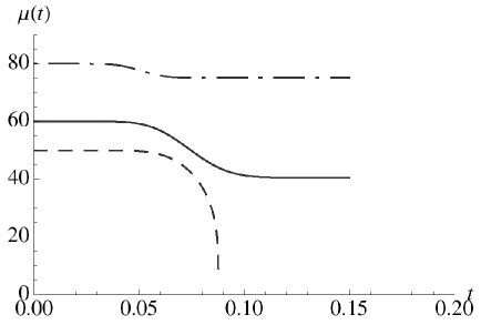
Figure 1: Evolution of velocity $\mu(t)$ of the colliding NRCO decelerating due to capture of the particles of the target. (Time and velocity are in dimensionless units.) Three initial velocities are considered: $\mu(0)_{A}=60$ units $=8\times 10^{6}\,m/s$ (solid line), $\mu(0)_{B}=80$ units (dash-dot line), and $\mu(0)_{C}=55$ units (dashed line).

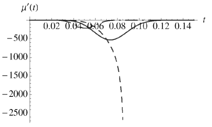
Figure 2: Evolution of deceleration rate (negative acceleration rate) $\mu^{\prime}(t)$ of the colliding NRCO decelerating due to capture of the particles of the target. (Time and deceleration rate are in dimensionless units.) Three initial velocities are considered: $\mu(0)_{A}=60$ units $=8\times 10^{6}\,m/s$ (solid line), $\mu(0)_{B}=80$ units (dash-dot line), and $\mu(0)_{C}=55$ units (dashed line).

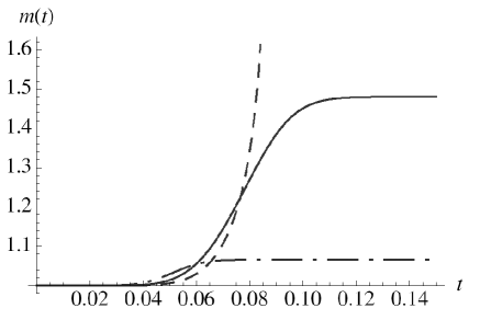
Figure 3: Evolution of mass $m(t)$ of the colliding NRCO decelerating due to capture of the particles of the target. (Time and mass are in dimensionless units.) Three initial velocities are considered: $\mu(0)_{A}=60$ units $=8\times 10^{6}\,m/s$ (solid line), $\mu(0)_{B}=80$ units (dash-dot line), and $\mu(0)_{C}=55$ units (dashed line).

In the base scenario (case A, solid line), during its flight, the colliding NRCO added more than 40% to its mass (Fig. 3) and lost about 1/3 of its speed (Fig. 1).

Case B (dash-dot line) corresponds to a higher initial velocity, which means that the duration of the fly-through is shorter and the number of captured particles involved in the process is smaller. This scenario has the least acquisition of mass (Fig. 3), the least loss of speed (Fig. 1), and the smallest maximum of the magnitude of deceleration (Fig. 2).

In Case C (dashed line) the NRCO completely stops (Fig. 1). It is important to keep in mind that such outcome should be considered as an asymptotic scenario. Our model is imprecise in the sense that the Bondi accretion interpolation formula assumes an infinite-sized nebula. Obviously, due to the law of mass conservation the NRCO cannot capture more than the mass of the target. Even if it captures a substantial portion of the target, the model become no longer accurate as it keeps constant certain properties of the target. Nonetheless, Case C shows that instant deceleration can reach enormous magnitudes (infinity at full stop) when mass acquisition is significant (Fig. 2).

An important general observation can be made from these simulations. The instantaneous deceleration magnitude can be rather large (even in the kinetic sense) when the NRCO can acquire enough (relative to itself) mass from the target. The absolute sizes of the colliding objects do not matter, only the relative do. Thus any of the above-mentioned target candidates (a planet, a dwarf, or the edge of the Sun) may be able to significantly decelerate the NRCO, if the NRCO has an appropriate size. (In Appendix B, we demonstrate that NRCOs of much smaller sizes than traditional neutron stars can indeed exist with the equation of state derived for this model.)

3.4 Density stratification

Strong deceleration leads to stratification of the NRCO’s core. Behavior of an elastic body in the frame of reference moving with acceleration/deceleration is analogous to its behavior in a homogeneous gravity field. This means that density stratification will always take place. This effect will be significant if the characteristic scale of stratification is much less than the size of the object. (The characteristic scale here is defined as $s^{2}/a$ where $s^{2}$ is square of the sound speed within the elastic body, and $a$ is deceleration magnitude).

In our scenario, significant stratification means $s^{2}/a\ll R_{nrco}$, where $R_{nrco}$ is the size of the NRCO. The magnitude of deceleration, $a$, may be estimated as $a\sim\Delta V/\tau$, where $\Delta V$ is the change of the NRCO’s velocity over the duration of the deceleration process, $\tau$. If NRCO deceleration is significant then $\Delta V$ is a meaningful fraction of $V$. The duration of the process (i.e., the duration of the flight through the target), $\tau$, may be estimated as $\sim R_{target}/V$, where $R_{target}$ is the size of the target. Thus, the condition for significant stratification becomes

$$\frac{s^{2}}{V_{nrco}^{2}}\ll\frac{R_{nrco}}{R_{target}}$$ (1)

Since in our case, $R_{nrco}\ll R_{target}$, it necessarily implies that for significant density stratification to take place, the elasticity of the NRCO matter (characterized by $s^{2}=\partial p/\partial\rho$) must become rather small, i.e. the mono-phase state of the matter has to be near the boundary of its thermodynamical (gas/liquid) equilibrium.

In Appendix B, we offer a model which possesses the necessary characteristics for such phenomenon. The NRCO’s core described by the equation of state (Eq. B11) can have quasi-homogeneous density distribution, except for a narrow region near the edge where density gradient is negative and extremely steep.

3.5 Explosion

As stated earlier, if the equilibrium state of the inner ”nuclear liquid” is initially close to the boundary of the liquid/gas phase transition, then decompression by deceleration can shift its phase state from the liquid phase into the two-phase zone of ”nuclear fog”. (We describe this process in detail in Appendix C.) In the two-phase zone, the matter can exist as a mixture of two phases of nuclear matter – either liquid droplets surrounded by gas of neutrons, or homogeneous neutron liquid with neutron- gas bubbles. In such state, the matter can reach substantial further rarification, reducing density by a factor of $10^{2}$ or more due to hydrodynamic instability. (See Appendix C.) Below density $\rho_{drip}$, beta-decays are no longer Pauli-blocked and significant amounts of energy become released. Indeed, in their simulations of $r$-process nucleosynthesis in neutron star mergers, Freiburghaus et al. (1999) observed that from the level of $\rho_{drip}$, the density dropped remarkably fast. The material initially cooled down by means of expansion, but then started to heat up again when the $\beta$-decays set in.

This energy, absorbed by the nuclear ”droplets” of the ”fog”, triggers fragmentation of these supersaturated hyper-nuclei (see Appendices B and C; see Bertsch et al. (1983), Heiselberg et al. (1988), Lopez et al. (1989)). These reactions, known to release even more energy ($\sim 1MeV$ per fission nucleon, as known from trans-uranium fission events), proceed effectively at the same time as the beta-decay reactions, all occurring with a very rapid nuclear time scale ($\sim 10^{-22}\div 10^{-15}\,sec$). When perturbations of the equilibrium of a neutron liquid (droplet) permit production of charged protons (even in small numbers, and in small localized regions), spontaneous fission reactions commence.

Fig. 4 (from Karnaukhov et al. (2011)) schematically explains the process. When a nuclei is excited weakly (low $T_{MeV}$), only $\gamma$-emission occurs. At a higher level of excitation, neutron-emissions start taking place. When even more energy is applied to the nucleus, it deforms and fission reactions start, because for deformed nuclei with $Z^{2}/A>50$, electrostatic repulsion starts exceeding surface tension. And finally, when injected energy is sufficiently high, splitting into fragments (”droplets” if the initial nucleus is a hyper-nucleus) occurs, followed by the cascade of further splitting into fragments and neutron emissions.

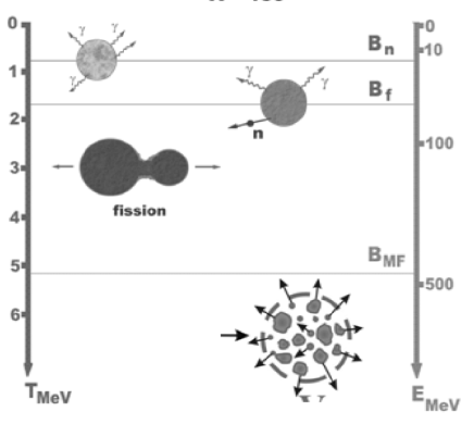
Figure 4: Types of nuclear reactions ($\gamma$-emission, neutron-emission, fission, multi-fragmentation) based on the injected energy of excitation. From Karnaukhov et al. (2011).

The energy released in the process can be powerful enough to crack the crust from within and eject a portion of the NRCO’s inner matter beyond its gravitational trap (see Section 3.1). Once ejected, the neutron ”droplets”, hyper-nuclei, and other components of the explosion, will transform into a variety of chemical elements.

3.6 Element production

Unfortunately, at this point it is not possible to assess the resulting abundances of the elements produced in the process.

First, the theory of fission (and even more so of fragmentation) of hyper-nuclei ($lnA\gg 1$) is not developed at all, mostly because observational data are impossible to collect. Fission reactions (split of elements with high $A$ numbers into several with lower $A$ numbers) lead to the unpredictable composition of the fission products, which vary in a broad probabilistic and somewhat chaotic manner. This distinguishes fission from purely quantum-tunnelling processes such as proton emission, alpha decay and cluster decay, which give the same products each time.

Second, while $r$-process production (from the lower to higher $A$ numbers) has been more studied and can be better modeled, the results strongly depend on the assumed equation of state (EOS) (Freiburghaus et al. (1999)), the neutron/seed ratio and the composition of the seed, which in models are characterized by the proton-to-nucleon ratio $Y_{e}$ of the ejected and expanding matter. The value of $Y_{e}$ has basically two effects: (1) It determines the neutron-to-seed ratio, which finally determines the maximum nucleon number $A$ of the resulting abundance distribution, and (2) it also determines the location (neutron separation energy) of the $r$-process path, and thus the $\beta$-decay half-lives encountered; this influences the process speed and the nuclear energy release. Thus, $Y_{e}$ of the ejected matter strongly depends on how much crust or core matter is contained in the ejecta. Also, various processes such as neutrino transport, neutrino captures, or positron captures, alter $Y_{e}$ evolution. In neutron star merger studies, test calculations using different polytropic EOSs indicate a strong dependence of the amount of ejecta on the adiabatic exponent of the EOS, where stiffer equations result in more ejected material. (Freiburghaus et al. (1999))

Finally, the data on the abundance yields from the observed supernovae are not useful for modeling the collision element production. The two processes (supernova and collision) fundamentally differ in several aspects. With respect to the nucleosynthesis reactions, the two explosions have substantially different seed nuclei composition and neutron-seed ratios. In supernova explosions, when the core collapses once coulomb repulsion can no longer resist gravity, the propagating outward shockwave causes the temperature increase (resulting from the compression) and produces a breakdown of nuclei by photodisintegration, for example: ${}^{56}Fe+\gamma\rightarrow 13^{4}He+4^{1}n$, ${}^{4}He+\gamma\rightarrow 2^{1}H+2^{1}n$. The abundant neutrons produced by photodisintegration are captured by those nuclei from the outer layers (the seeds ) that managed to survive. Thus, the produced abundances depend strongly on the characteristics of the star. Indeed, astronomical observations confirm that supernova nucleosynthesis yields vary with stellar mass, metallicity and explosion energy (see, for example, Nomoto et al. (2006)). In comparison, the NRCO has no outer layers (other than $Fe$ crust) and thus does not follow the same, as in supernova, chain of photodisintegration reactions to supply the seeds and the free neutrons. On the other hand, in the collision, a completely different from supernova distribution of seeds is supplied by the nuclei from the target. But most importantly, in the collision scenario, reactions of fission, rather then nucleosynthesis, play the dominant role in the element production.

The only thing that can be said at this point is that, in the framework of the outlined hypothesis, the observed abundances of the solar system represent the only outcome of such collision event known to us (of course, the final abundances also include contributions from stellar and in situ sources). We do not have a statistical sample to make any comparisons. If the fission and nucleosynthesis reactions were better understood, the only subsequent approach would have been to solve the inverse problem, i.e. to find out what the initial conditions had to be so the model resulted in the observed abundances.

3.7 Probability of another collision event

We suspect that the collision event proposed in our scenario is a unique and extraordinary event. The only reason it was even envisioned is because many existing characteristics of the solar system are otherwise difficult to explain self-consistently (see Section 1.1).

To get a feel for how likely a similar event can be, we estimate the time of a collision of an object with a target (star): $\tau\sim L^{3}/(\pi R^{2}\times V$ ), i.e., space volume per star / ( target cross-section $\times$ approach velocity). In the Sun’s neighborhood, the average distance between the stars is roughly 5 light years ($L=5\times 10^{13}km$). Near the core of the Galaxy, stars are packed fairly tight, about 1/4 light year apart. Because of gravity interaction, the paths of stars that would have missed each other will curve toward each other and have a grazing collision even when their trajectories looked like they would miss initially, thus increasing the capture cross-section. So let us assume that the effective size of the collision target is of order of $R\sim 10^{6}\,km$. Finally, assume the approach velocity $\sim 10^{3}\,km/s$. Thus, the characteristic time for one particular neutron star to collide with a star as

$$\tau_{1}\sim\frac{(5\times 10^{13}\,km)^{3}}{3.14\times(10^{6}\,km)^{2}\times 10^{3}\,km/s}\sim 10^{18}yrs.$$

Some astrophysicists estimate that there may be as many as $10^{8}$ neutron stars in our Galaxy. (Kutschera, 1998) Furthermore, non-rotating and non-accreting neutron stars which have cooled down are virtually undetectable by conventional means. Gravitational micro-lensing experiments have detected a population of such objects in the galactic halo. These stars have sufficiently high initial velocity. (Kutschera, 1998)

Using the estimate of $10^{8}$ neutron stars, we estimate the probability of a collision of some neutron star with some planetary system in our galaxy as

$$1/\tau=N\times 1/\tau_{1}\sim 10^{8}stars\,/10^{18}yr\,\sim 10^{-10}yr^{-1}.$$

Which means that this kind of a collision is indeed a very rare event, with the odds of being ”once in a lifetime” (the lifetime of the Universe so far is $\sim 1.34\times 10^{10}$ years).

This result also implies that the exoplanetary systems are most likely formed according to the ”normal” processes of planet formation. In the framework of our hypothesis, the ”rocky” exoplanets most likely will not have the same composition as our terrestrial planets. Data on the actual differences would provide valuable insights into the validity of our hypothesis. Unfortunately, at this point, the measurement techniques employed to detect exoplanets are not yet capable of determining what the exoplanets are actually composed of.

4 Summary

We advanced a hypothesis that the early solar system (initially possessing no terrestrial planets) became enriched with the observed and extinct $r-$, $s$-, and $p$-process elements predominantly as a result of its collision with a neutron star-like object (a ”neutron-rich compact object”, or NRCO). These elements subsequently formed dust grains, accreted into larger and larger rocky bodies, and eventually formed the modern terrestrial planets.

To eject its neutron-rich core matter into the solar system and produce the chemical elements via complex chains of nuclear reactions, the NRCO had to explode, at least partially. We identified that the key mechanism leading to the explosion was density decompression and subsequent nuclear reactions in the back of the NRCO’s core, which resulted from the straight-line deceleration of the NRCO as it penetrated a dense massive solar system body located within the zone of current terrestrial planets. (Such straight-line deceleration and subsequent decompression do not occur in the familiar stellar events, such as supernova or neutron star mergers, and therefore has never been examined before.)

As established in nuclear physics, in the phase state of ”nuclear fog” – where nuclear liquid and gas co-exist – density decrease by a factor of $10^{2}$ or more can indeed take place. From this perspective, in our model the ”strength” of the NRCO’s deceleration becomes then defined not in the kinetic sense, but in the thermodynamic sense. If the initial phase state of the neutron liquid is rather close to the boundary of the unstable two-phase zone, even a small deceleration magnitude in the kinetic sense, can still trigger sufficient density decompression. In the unstable zone, density perturbations develop exponentially fast. Furthermore, nuclear reactions occur with even faster time scales ($t\sim 10^{-22}\div 10^{-15}$ sec). Thus, even a short-lived localized fluctuation of density to below $\rho_{drip}$ can trigger the cascade of nuclear reactions. Recent findings from the high-density / high-energy nuclear physics established that nuclear reactions of multi-fragmentation of hyper-nuclei and fission of super-nuclei are capable of releasing sufficient amounts of energy, which is needed for the explosion and ejection of the NRCO’s core matter against its gravitational pull.

At this point, we have not established many constraints on the nature of the target. Its only critical characteristic so far is that it must have been able to sufficiently decelerate the NRCO. From this perspective, the target could have been a ”super-Jupiter” rotating on the first orbit (i.e., between the Sun and Jupiter, as no terrestrial planets existed at that time), or a close binary companion of the Sun (if such existed), or the edge of the Sun (if the collision could occur without destroying the Sun). If the target was the ”super-Jupiter” or the Sun’s companion, its current absence implies that it was either destroyed or ejected as a result of the collision.

With respect to the NRCO, our model requires a priori only that it contains dense neutron liquid in its core and has a solid crust (as do neutron stars), and has such other characteristics that in the collision its density (in a localized spot) decompresses to the level when nuclear reactions can cascade. For example, the NRCO has to travel fast enough, so the collision has a ”head-on”, straight-line type deceleration, to create decompression in the back. In our analysis, we considered the acquisition of the target mass by the NRCO as the primary deceleration mechanism, which therefore required that the NRCO be gravitationally-powerful and sized in such a way relative to the target, so the target had enough mass to decelerate the NRCO. In general, other mechanisms of deceleration (interaction of magnetic fields, for example) may also play significant if not dominant role. Overall, however, it is the aggregate deceleration magnitude that is crucial, regardless of which mechanism is dominant. The closer the NRCO’s initial equation of state (EoS) is to the liquid/gas phase-transition boundary, the smaller the deceleration magnitude is required for the sufficient decompression and subsequent nuclear reaction cascade. (We demonstrated that NRCO’s with such characteristics can theoretically exist, and even have smaller sizes than traditional neutron stars. Therefore, the role of NRCO can be played perhaps by a piece of a neutron star, torn apart and catapulted by a distant black hole.)

Once a portion of the NRCO’s core matter is ejected into the solar system, two main element production mechanisms take place: multi-fragmentation/ fission (split of nuclei with high $A$ numbers into several with lower $A$ numbers), and nucleosynthesis (formation of elements by nucleon capture from lower to higher A numbers). In the collision scenario, hyper-nuclei fragmentation/ fission are most likely dominant. (In supernova, nucleosynthesis is the main mechanism.)

Unfortunately, a more detailed analysis is constrained by the limitations in the current understanding of (1) the EoS of high-density nuclear matter and (2) the nuclear reactions for hyper- and super-nuclei. While significant advances have been made by nuclear physicists in recent years, further developments of theory and additional experimental data are needed. Therefore, we cannot at this point estimate the energy or mass of the ejecta, nor the produced abundances of the elements, nor the implications for the orbital dynamics of the solar system objects, nor the fate of the colliding objects. Nonetheless, the proposed hypothesis presents a new framework from which the entire evolution of the solar system can be re-evaluated.

The collision hypothesis has the advantage over all other currently considered theories (among which the supernova enrichment theory being one of the most commonly accepted so far), because the collision scenario is capable of self-consistently explaining all cosmo-chemical inconsistencies (see Section 1.1) by invoking only one event. It is theoretically apparent that an ejecta of super-hot neutron-rich hyper-nuclei into the surrounding medium from the target, can produce every chemical element ever detected in the solar system. The planetary structure of the solar system (with two classes of planets and atypically wide, circular and non-resonant orbits of giants) also fits better within the collision scenario. Finally, the collision hypothesis does not contradict any of the already developed theories, but rather integrates them all from a different perspective. For example, all of the stellar enrichment models are valid conceptually, but the relative contributions from various mechanisms perhaps is less than have been assumed so far.

Appendix A Brief overview of models of equations of state for nuclear matter and neutron stars

As examples, we list several models of equation of state for dense matter.

Particles with interaction

Equations of state obtained from a Yukawa-type interaction in the Hartree–Fock approximation are (see (Shapiro, Teukolsky, 1983), p. 217)

$$\rho=nm+\frac{3}{10}(3\pi^{2})^{2/3}\frac{\hbar}{mc^{2}}n^{5/3}\pm\frac{\pi g^{2}}{\mu^{2}c^{2}}n^{2},$$

$$p=Kn^{5/3}\pm\frac{\pi g^{2}}{\mu^{2}}n^{2}$$ (A1)

Here, $\mu=\hbar/m_{g}c^{2}$ is the inverse of the Compton wavelength of the $g$-field quanta, $g$ is the ”charge” of the Youkawa–like interaction. Condition $\mu\sim 1.46\,fm$ ($1\,fm=10^{-15}\,m$) requires the field quanta ($\pi$-meson) to have a mass $\sim 140\,Mev$ (i.e. comparable to pion mass). The experimental data give $g^{2}/\hbar c\sim 10$. For $W$-boson (weak-interactions) $\mu_{W}\simeq 2.45\times 10^{-18}\,m$. For nucleon $\mu_{p}\simeq 1.32\,fm$.

For high densities, the equation of state is hardened due to the dominance of the ”repulsive core” Yukawa potentials. As $n\rightarrow\infty$, the equation of state satisfies (ibid, p. 211) $p\rightarrow\rho c^{2}.$ The sound speed approaches in this case $c_{s}=(\partial p/\partial\rho)^{1/2}\rightarrow c$, in contrast to an ideal relativistic gas, for which $p\rightarrow 3^{-1}\rho c^{2}$ with $c_{s}\rightarrow 3^{-1/2}c.$

The Bethe-Johnson equation of state (ibid, p. 221), as an example of a variational calculation, proposes the equation of state

$$p=n^{2}\frac{\partial}{\partial n}(\frac{\epsilon}{n})=364\,n^{a+1}\,Mev\,fm^{-3}$$

$$\quad\mbox{with}\quad c^{2}_{s}=\frac{n^{a}}{1.01+0.648n^{a}}c^{2},$$ (A2)

where $a=1.54,\;0.1\leq n\leq 3\;fm^{-3}$ or $1.7\times 10^{14}\leq\rho\leq 1.1\times 10^{16}\,g\,cm^{-3}$. Obviously, a causality violation exists, $p>\rho c^{2}$, at high densities.

Like all many-body calculations of the equation of state, the Bethe-Johnson calculation is by no means the final word on the issue (ibid, p. 224).

Super-dense substances

The inner core composition of a neutron star is not exactly known due to insufficient knowledge of the physics of strong interactions in super-dense substances (Fortov, 2009). It is not unlikely that the core consists of a nucleon-hyperon substance, pion condensate, quark-gluon plasma, or some other exotic states. According to some authors, if the properties of the neutron star crust ($\rho<0.5\rho_{0}$) are relatively well described by non-ideal plasma models, then for $\rho>5\rho_{0}$ the description of the properties of a super-nuclear-density substance is severely hampered by both the incompleteness of laboratory data and the absence of a complete theory of super-nuclear-density substances.

Quark-gluon plasma

From (Fortov, 2009): ”Quark-gluon plasma [184 - 187] constitutes the super-hot and super-dense form of nuclear matter with unbound quarks and gluons which are bound inside hadrons at lower energies (Figs 13a and 13b). The existence of QGP follows from the property of asymptotic freedom of QCD [188 - 191], which yields a value of $1-10\,GeV/fm^{3}$ for the energy density of a corresponding transition (recall that $1\,\Gamma ev$ is approximately a mass of a nucleon, $m_{p}=931\,Mev$, and $1\,fm=10^{-13}cm$). Detailed numerical calculations give the critical conditions for the emergence of QGP: $T^{qg}_{c}\simeq 0.15-0.2\,\Gamma eV$, or $T^{qg}_{c}\simeq(1.8-2.4)\times 10^{12}\,K$ (Figs 13d and 13f).

The initiation of this plasma manifests itself in an increase in the number of degrees of freedom - from three inherent in the pion gas at low temperatures, $T<T^{qg}_{c}$, to $40-50$ inherent in the QGP for $T>(1-3)T^{qg}_{c}$. Since the energy density, the pressure, and the entropy are approximately proportional to the excited degrees of freedom of the system, a sharp variation in these thermodynamic parameters in a small vicinity of $T^{qg}_{c}$ accounts for the large energy difference between the ordinary nuclear substance and the QGP. Like our customary ”electromagnetic” plasma, QGP may be ideal for $T\gg T^{qg}_{c}$, and nonideal for $T\simeq(1-3)T^{qg}_{c}$. The corresponding nonideality parameter - the ratio between the inter-particle interaction energy and the kinetic energy $E_{c}in$ in this case is given in the form $\Gamma\simeq g^{2}/aT$, where numerical constants of order unit are omitted, the inter-particle distance $a\sim T^{-1}\;(a\sim 0.5\,fm,\;T=200eV)$, and the strong interaction constant $g\sim 2$”.

Appendix B VdW–like equation of state

As mentioned in Section 2.1, the involved in the proposed collision NRCO must have been compact and gravitationally-powerful to contain in its interior the highly dense neutron fluid (which is necessary for the eventual formation of the intermediate and heavy elements). Various models for the equation of state have been proposed (for neutron stars), but their reliability decreases with growing density, because the precise relativistic many-body theory of strongly interacting particles is not fully developed.

Thus, in order to study the collision process, for the model of the NRCO we use the Skyrme-like approach. This approach (common in nuclear physics) describes pair-interactions of particles whose mutual attraction is taken into consideration, as well as the existence of repulsing core within the particles. The approach also assumes the validity of the following invariances: translation, Galilean, rotational, isospin, parity, and time-reversal. Moreover, some terms are added that cannot be derived from the invariance argument, e.g., spin-orbit interaction, or the 3-body-type medium effect.

Essentially, the particle interaction is described by density. This framework is expected to represent the collective dynamics. As a result, the equation of state for the system may be similar to Van der Waals (VdW) model due to their observed similarity (Karnaukhov, 2006).

B.1 Theoretical concept

For such a model, the free energy of the system is given by

$$F(\rho,T)=A+\frac{3}{8}\xi\bigg{(}-\frac{8}{3}T\ln\bigg{[}T^{3/2}\frac{(3-\rho)}{3\rho}\bigg{]}-3\rho\bigg{)},$$ (B1)

where $\xi$ and $A$ are constants. Knowing free energy, pressure $p(\rho,T)=\rho^{2}\partial_{\rho}F(\rho,T)$ can be determined from the thermodynamical equality $dF=-sdT-pd(\rho^{-1})$:

$$p(\rho,T)=\frac{3}{8}\xi\bigg{(}\frac{8\rho T}{3-\rho}-3\rho^{2}\bigg{)}.$$ (B2)

This is the VdW interpolation equation of the state, where the dimensionless quantities $p,\rho$ and $T$ are pressure, density and temperature normalized by the critical values $\rho_{c},\,T_{c}$ and $p_{c}$, whose existence follows from the given form of the free energy. The critical density is determined from the conditions $(\partial_{\rho}p)_{c}=0$ and $(\partial_{\rho\rho}p)_{c}=0$. The critical parameters are not independent and are related by the relation $p_{c}/\rho_{c}=(3/8)c^{2}(T_{c}/m_{N}c^{2})\equiv(3/8)c^{2}\xi$, where $c$ is the light speed, temperature $T_{c}$ is measured in energetic units, $m_{N}$ represents the mass of a particle of the system. Dimensionless parameter $\xi=(T_{c}/m_{N}c^{2})\ll 1$.

The meaning of the expressions (B1) and (B2) is as follows: In classical gases under normal conditions, interaction between particles (molecules, atoms) is weak. As the interaction (pressure) increases, the properties of the system differ more and more from the properties of the ideal gas, and finally the gas enters its condensed state – liquid. In the liquid state, interaction between particles is great, and properties of this interaction strongly depend on the specific type of the liquid. This is the reason why general formulae, describing quantitatively properties of liquids, do not exist (see Landau, Lifshitz (1969)–Landau, Lifshitz (1987)).

However, it is possible to find some interpolation formula which can qualitatively describe the transition between the gas and liquid (as done in the Van der Waals model). Such formula must produce correct results in two limit cases. For rarified gases, it should converge into formulae correct for ideal gases. But as the density increases, it should incorporate the fact that the compressibility of the matter is limited. Such formula then would qualitatively describe the gas behavior in the transition state.

Expression (B1) satisfies such conditions. At low densities, $\rho\ll 3$, Eq. (B1) becomes the expression for the free energy of the ideal gas; at large densities $\rho\rightarrow 3$, it shows that unlimited gas compression is impossible (at $\rho>3$, the argument in the logarithm is negative; it is also obvious that $\rho$ cannot be negative.)

Eq. (B1) represents only one of the numerous possible interpolation formulae satisfying the posed requirements. There are no physical reasons to prefer one such interpolation over the others. But the VdW form (Eq. B1) is one of the simplest and easiest to work with.

The nucleon-nucleon interaction is composed of two components: a very short-range repulsive part and a long-range attractive part. The nuclear interaction is similar to VdW- interaction within a molecular medium. In a sense, the phase transition in nuclear matter resembles the liquid-gas phase transition in classical fluids. However, as compared to classical fluids the main difference comes from the gas composition: for nuclear matter, the gas phase is predicted to be composed not only of single nucleons, neutrons and protons, but also of complex particles and fragments depending on temperature conditions.

According to Silva et al. (2004) and Goodman et al. (1984), the nuclear equation of state (EOS) can be presented as follows:

$$p=a\rho-b\rho^{2}+c\rho^{3},$$ (B3)

where $a=k_{B}T,\,b=k_{B}T_{c}/\rho_{c}$ and $c=2k_{B}T_{c}/6\rho_{c}^{2}$. The coefficients $b$ and $c$ depend directly on the value of the critical temperature $T_{c}$ and the critical density $\rho_{c}$.

A typical set of isotherms for an equation of state (EoS) - pressure versus density with a constant temperature - corresponding to nuclear interaction (Skyrme effective interaction and finite temperature Hartree-Fock theory, see Jaqaman et al. (1983)) is shown in Fig. 5.

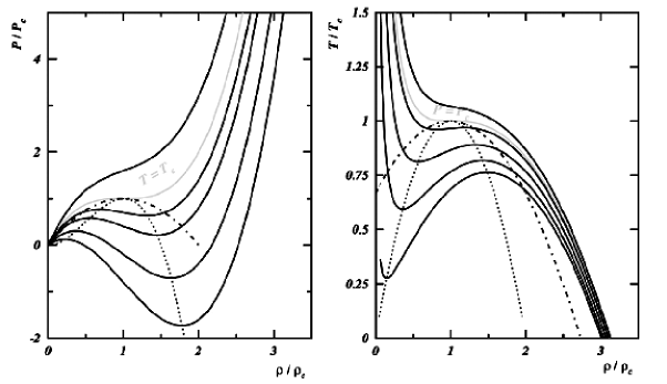
Figure 5: Equation of state for nuclear matter: pressure (isotherms, left panel) or temperature (isobars, right panel) as functions of density. (Parameters are normalized to their critical values). The dash-dotted lines are the coexistence lines, the dotted lines are the spinodal lines. From Borderie (2002). See also, Borderie Rivet (2008).

It exhibits the maximum-minimum structure typical of the VdW–like EoS. Depending on the effective interaction chosen and on the model (see Jaqaman et al. (1983), Jaqaman, et al. (1984), Csernai (1986), Muller et al. (1995)), the nuclear equation of state exhibits a critical point at $\rho_{c}\simeq(0.3\div 0.4)\rho_{0}$ and $T_{c}\sim 5\div 18\,MeV$ (Cherepanov, Karnaukhov (2009), Karnaukhov et al. (2011)). Calculations of $T_{c}$ were performed in Silva et al. (2004), Goodman et al. (1984), Sauer et al. (1976), Jaqaman et al. (1983), Zhang (1996), Taras et al. (2004). Experimental data are presented in Fig. 6.

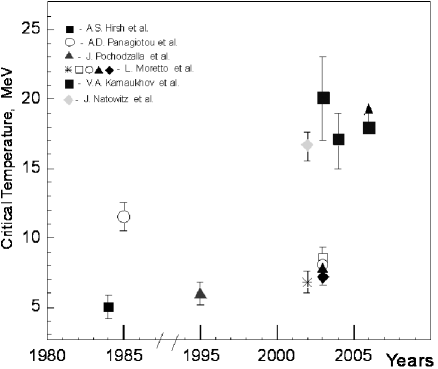
Figure 6: Values of critical temperatures of nuclei $T_{c}$ measured by different techniques. From Karnaukhov et al. (2011).

In Fig. 5, $\rho_{0}$ refers to normal density. The region below the dotted line in Fig. 5 corresponds to a domain of negative compressibility: here, at constant temperature, an increase of density is associated with a decrease of pressure. Therefore in this region a single homogeneous phase is unstable and the system falls into a liquid-gas phase in equilibrium. It is the so-called spinodal region, and spinodal instability produces breaking into the two phases. Such instability has been proposed, for a long time, as a possible mechanism responsible for multi-fragmentation (Bertsch et al. (1983), Heiselberg et al. (1988), Lopez et al. (1989)). The spinodal region constitutes the major part of the coexistence region (dashed–dotted line in Fig. 5) which also contains two meta-stable regions: one at density below $\rho_{c}$ for the nucleation of drops and one above $\rho_{c}$ for the nucleation of bubbles (nuclear cavitation). The boiling temperature for nuclear matter is $\sim 3$ times less then the critical temperature ($T_{b}\sim 6MeV$, $T_{c}\sim 18MeV$, see Karnaukhov et al. (2011)).

The hot piece of nuclear matter produced in any nuclear collision has at most a few hundred nucleons $A\sim 200$ and so is not adequately described by the properties of infinite nuclear matter (or with $\ln\,A\gg 1$) where surface and Coulomb effects can not be ignored. These effects can lead to a sizable reduction of the critical temperature.

Experimentally, it was shown that in a collision $p+Au$, first a combined excited nucleus is formed. The excitation energy is distributed between the thermal, compressional, and rotational (for heavy ions) energies. For colliding protons with initial $E=8.1\,MeV$, i.e., $T\sim 5-7\,MeV$, the thermal energy component is $E_{th}>400\,MeV$. The nucleus ”boils up” (see Karnaukhov et al. (2011); Pavlov, Kharin (1990)), and multi-fragmentation ($m$ fragments with $Z\sim(2-20)$) and emission of protons and neutrons take place.

B.2 Interpolating model of EoS

The high density of the NRCO’s nuclear matter requires that the VdW-like equation of state (EoS) be expanded into the relativistic domain. When $\rho\rightarrow 3$, the speed of sound, in the framework of model Eq. (B2), tends to infinity, which is impossible because the sound speed is always less then speed of light. For this reason, we require that the equation of state for the NRCO matter is analogous to the EoS of the VdW gas for small $\rho<3$, but produces in the relativistic density domain ($\rho\gg 3$) the sound speed equal to $1/\sqrt{3}$ (appropriate for the gas composed of free relativistic particles). Then, the interpolation formula for the free energy can be proposed in the form

$$F(\rho,T)=$$

$$\bigg{(}A+\frac{3}{8}\xi(-\frac{8}{3}T\ln[T^{3/2}\frac{(3-\rho)}{3\rho}]-3\rho)\bigg{)}\theta[3-x-\rho]+$$

$$\frac{1}{3}\bigg{(}-\ln\frac{1}{\rho}-\frac{\alpha}{\rho}-\frac{\beta}{\rho^{2}}-\frac{\gamma}{\rho^{3}}\bigg{)}\theta[\rho-3+x].\quad$$ (B4)

Here, $\theta[s]$ is the Heaviside step–function, $\theta[s]=1$ when $s>0$ and $\theta[s]=0$ when $s<0$; free parameters $A,\alpha,\beta,\gamma,x$ assure the continuity of free energy $F$; pressure $p=\rho^{2}\partial_{\rho}F$; sound speed (squared) $s^{2}=\partial_{\rho}p$. Parameter $x$ represents the transition point between relativistic and non-relativistic domains in the expression defining the free energy $F$.

In the domains of small and large densities, the speed of sound (squared) takes form:

$$(s_{-}^{2})\equiv s^{2}\bigg{|}_{\rho<3-x}=\frac{3T\xi}{3-\rho}-\frac{9\xi\rho}{4}+\frac{3T\xi\rho}{(3-\rho)^{2}},$$ (B5)

$$(s_{+}^{2})\equiv s^{2}\bigg{|}_{\rho>3-x}=6\frac{\gamma}{\rho^{4}}+4\frac{\beta}{3\rho^{3}}.$$ (B6)

Derivative $\partial(s_{-}^{2})$, obtained from Eq. (B5), gives

$$\partial_{\rho}(s_{-}^{2})=-\frac{9\xi}{4}+\frac{6T\xi}{(3-\rho)^{2}}-\frac{6T\xi\rho}{(3-\rho)^{3}}$$ (B7)

Eqs.(B4)-(B7) form the system of equation which allows derivation of the EoS $p(\rho,t)$. Because this system cannot be solved analytically, we solve it numerically and present results for one set of representative initial parameters.

For the following numerical example, we take values of $\xi=0.007$ and $T=0.1$, which are within their commonly assumed ranges, but allow us to produce illustrating figures with good visual resolution.

Next, we take small $(s_{-}^{2})=10^{-2}$ (i.e. the matter is near the phase transition boundary but is still in its liquid state) and replace $\rho\rightarrow 3-x$. We find then that $x=0.3489$ and $\partial_{\rho}(s_{-}^{2})=0.2809$. Then

$$(s_{+}^{2})=\frac{1}{3}-0.0949\beta-0.1074\gamma.$$ (B8)

$$\partial_{\rho}(s_{+}^{2})=0.0716\beta+0.1215\gamma.$$ (B9)

Because the values of $s_{\pm}^{2}$ and of their derivatives are by definition the same at the transition point $x$, we can then solve for $\beta=2.3745$ and $\gamma=0.9140$. Therefore, the interpolation formula for the square of sound speed $s_{+}^{2}$ becomes

$$s^{2}=\bigg{(}\frac{0.0021}{(3-\rho)}-0.0158\rho+(\frac{0.0021\rho}{(3-\rho)^{2}}\bigg{)}\theta[2.6511-\rho]$$

$$+\bigg{(}\frac{1}{3}-\frac{1.8280}{\rho^{3}}-\frac{1.5830}{\rho^{2}}\bigg{)}\theta[-2.6511+\rho].\quad$$ (B10)

Parameters $A$ and $\alpha$ are found from the continuity condition for the free energy and the pressure, resulting in $A=-0.1423(-1.4921+0.8837\alpha)$ and $\alpha=-4.9507$. Thus, the final expression for the equation of state (EoS) becomes

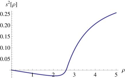
Figure 7: Dimensionless sound speed within the nuclear matter, $s^{2}(\rho)$, calculated for initial temperature $T=0.1$. When $\rho\rightarrow\rho_{0}\simeq 2.6$, the sound speed in the matter tends to zero. For $\rho<2.6$, the system becomes unstable with respect to small fluctuation, and transits to two–phase state.

$$p(\rho,T=0.1)=\bigg{(}\frac{0.0021\rho}{3-\rho}-0.0079\rho^{2}\bigg{)}\theta[2.6511-\rho]+$$

$$\bigg{(}\frac{\rho}{3}-1.6502+\frac{1.5830}{\rho}+\frac{0.9140}{\rho^{2}}\bigg{)}\theta[-2.6511+\rho]\bigg{)}.\quad$$ (B11)

Obviously, Eqs. (B10) and (B11) can be generalized for arbitrary temperatures.

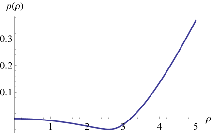
Figure 8: Dimensionless pressure.

B.3 Radially-symmetrical distribution of mass

To apply this framework to the spherical NRCO, first we demonstrate that the spherical configuration can indeed exist with the above-derived equation of state (VdW-like EoS with relativistic extension).

We introduce quantity $m$ (here defined in usual units, but later normalized) which has the meaning of the ”mass inside radius $r$”:

$$m(r)=4\pi\int_{0}^{r}drr^{2}\rho.$$ (B12)

The total NRCO mass, $M$, is the integral of (B12) from $0$ to $R$, and includes all contributions to the mass including gravitational potential energy: in fact, the proper volume element in the gravity field is not $4\pi r^{2}dr$ but $4\pi r^{2}g_{rr}^{1/2}dr=4\pi r^{2}(1-2m/r)^{-1/2}dr$. When $r\rightarrow R$, $m$ must become equal to $M$, so that the interior metric matched smoothly the exterior Schwarzschild metric. (Shapiro, Teukolsky (1983))

The equilibrium configuration is found from the Gilbert-Einstein’s equations (Oppenheimer–Volkoff equations) written as

$$\frac{dm}{dr}=4\pi r^{2}\rho,$$ (B13)

$$\frac{dp}{dr}=-G\frac{m\rho}{r^{2}}(1+\frac{p}{c^{2}\rho})(1+4\pi\frac{pr^{3}}{mc^{2}})(1-2\frac{Gm}{c^{2}r})^{-1},$$ (B14)

$$\frac{d\Phi}{dr}=-\frac{1}{\rho}\frac{dp}{dr}(1+\frac{p}{c^{2}\rho})^{-1}.$$ (B15)

Terms $\sim c^{-2}$ and $\sim G/c^{2}$ describe corrections produced by effects of the special and general theories of relativity.

Introducing dimensionless variables $r\rightarrow R_{*}r,\;\rho\rightarrow\rho_{c}\rho[r],\;m\rightarrow\rho_{c}R_{*}^{3}m[r]$, we obtain that the (now dimensionless) quantity $m[r]$ and its boundary condition become

$$m[r]=4\pi\int_{0}^{r}drr^{2}\rho[r]$$ (B16)

and

$$m[1]=\mu\frac{M}{R^{3}}.$$ (B17)

Here mass and radii are measured in the units of the Sun (denoted $\odot$), $M=M_{*}/M_{\odot}$, $R=R_{*}/R_{\odot}$, $M_{\odot}$ and $R_{\odot}$ are respectively the mass and radius of the Sun, dimensionless parameter $\mu=M_{\odot}/\rho_{c}R_{\odot}^{3}$. Numerically $\mu=1.45\times 10^{-13}$ if $\rho_{c}=0.4\times 10^{17}\,kg/m^{3}$.

Now we transform Eq. (B14) to the form convenient for calculations

$$\frac{dp[r]}{dr}=-\frac{G\rho_{c}^{2}R_{*}^{4}}{p_{c}R_{*}^{2}}\frac{m[r]\rho[r]}{r^{2}}(1+\frac{p_{c}}{c^{2}\rho_{c}}\frac{p[r]}{\rho[r]})\times$$

$$(1+\frac{4\pi p_{c}R_{*}^{3}}{\rho_{c}R_{*}^{3}c^{2}}\frac{p[r]r^{3}}{m[r]})(1-\frac{2G\rho_{c}R_{*}^{3}}{c^{2}R_{*}}\frac{m[r]}{r})^{-1},$$ (B18)

i.e.

$$\frac{dp[r]}{dr}=-\chi R^{2}(\frac{c^{2}\rho_{c}}{p_{c}})\frac{m[r]\rho[r]}{r^{2}}(1+(\frac{p_{c}}{c^{2}\rho_{c}})\frac{p[r]}{\rho[r]})$$

$$\times(1+4\pi(\frac{p_{c}}{\rho_{c}c^{2}})\frac{p[r]r^{3}}{m[r]})(1-2\chi R^{2}\frac{m[r]}{r})^{-1}.\quad\quad$$ (B19)

The universal coefficient $\chi=G\rho_{c}R_{\odot}^{2}/c^{2}=1.4623\times 10^{9}$. Parameter $\xi=T_{c}/m_{N}c^{2}$ varies from $0.005$ to $0.02$ depending on the assumed $T_{c}$. We use $\xi=0.007$.

The resulting mass and pressure distributions are:

$$\frac{dm[r]}{dr}=4\pi r^{2}\rho[r],$$ (B20)

$$\frac{dp[r]}{dr}=-\frac{8}{3\xi}\chi R^{2}\frac{m[r]\rho[r]}{r^{2}}(1+\frac{3}{8}\xi\frac{p[r]}{\rho[r]})$$

$$\times(1+\frac{3\pi}{2}\xi\frac{p[r]r^{3}}{m[r]})(1-2\chi R^{2}\frac{m[r]}{r})^{-1}.$$ (B21)

Together with Eqs. (B10) and (B11) for the EoS and the sound speed, they complete the system of equations from which a radially-symmetrical distribution of mass within the NRCO can be found. These equations cannot be resolved analytically in a general form. But their linearized version can be analytically solved (see next section).

B.4 Analytical solution

To linearize Eqs. (B20) and (B21), we write $\rho[r]=\rho[1]+\eta[r]$ and $m[r]=\frac{4\pi}{3}\rho[1]r^{3}+\mu[r]$. Quantities $\eta[r]$ and $\mu[r]$ may be considered as ”add-ons”, small perturbations of the basic state. The boundary conditions are $\eta[1]=0$ and $\mu[0]=0$. After substitution of these expressions into Eq. (B21), we obtain the set of equation for the normalized density add-on $\eta[r]$ and mass add-on $\mu[r]$, in the linear approximation,

$$\frac{d\mu[r]}{dr}-4\pi r^{2}\eta[r]=0,$$ (B22)

$$-\frac{2\beta_{-6}\kappa R_{-6}^{2}r\eta[r])}{(1-\beta_{-6}R_{-6}^{2}r^{2})}+\frac{d\eta[r]}{dr}=-\frac{\alpha R_{-6}^{2}r}{(1-\beta_{-6}R_{-6}^{2}r^{2})}$$

$$-\frac{\lambda R_{-6}^{4}}{(1-\beta_{-6}R_{-6}^{2}r^{2})^{2}}\mu[r]-\frac{\nu R_{-6}^{4}}{r^{2}(1-\beta_{-6}R_{-6}^{2}r^{2})}\mu[r].$$ (B23)

Here, we used symbolism $R=10^{-6}R_{-6}$ for notation brevity. For $T=0.1$, $\xi=0.007$, $\chi=1.4623\times 10^{9}$, and boundary conditions

$$m[1]=1.45\times 10^{-13}\frac{M}{R^{3}},\quad\rho[1]=3.1970\leftarrow p[1]=0.\quad$$ (B24)

numerical constants become $\alpha=1.95\times 10^{2}$, $\beta_{-6}=3.92\times 10^{-2}$, $\lambda=0.57$, $\kappa=7.78\times 10^{2}$ and $\nu=1.45\times 10^{1}$. In Eq. (B23), we neglected nonlinear terms of order $\eta^{2}$, $m^{2}$ and $\eta\,m$. The square of sound speed in this state is $s^{2}\simeq 0.12$.

The set of Eqs. (B22) and (B23) for the normalized density add-on and mass add-on, produces the general solution which satisfies the boundary condition only if $R_{-6}^{2}<\beta_{-6}^{-1}\simeq 25.5327$, i.e., radius $R_{-6}$ must satisfy condition $0<R_{-6}<5.0530$. Thus, the normalized density add-on $\eta[r]$ can be expressed as

$$\eta[r]=$$

$$\frac{\alpha R_{-6}^{2}}{(1-\beta_{-6}R_{-6}^{2}r^{2})^{\kappa}}\int_{r}^{1}ds\,s(1-\beta_{-6}R_{-6}^{2}s^{2})^{\kappa-1}+$$

$$\frac{\nu R_{-6}^{2}}{(1-\beta_{-6}R_{-6}^{2}r^{2})^{\kappa}}\int_{r}^{1}\frac{ds}{s^{2}}(1-\beta_{-6}R_{-6}^{2}s^{2})^{\kappa-1}\mu[s]+$$

$$\frac{\lambda R_{-6}^{4}}{(1-\beta_{-6}R_{-6}^{2}r^{2})^{\kappa}}\int_{r}^{1}ds(1-\beta_{-6}R_{-6}^{2}s^{2})^{\kappa-2}\mu[s].$$

(B25)

Quantity $\mu[r]$ satisfies the integral equation written here in the symbolic form

$$\mu[r]=(\frac{4\pi}{3}\alpha R_{-6}^{2})f[r]+$$

$$(\frac{4\pi}{3}\nu R_{-6}^{2})\widehat{G}_{1}[r,s]\mu[s]+(\frac{4\pi}{3}\lambda R_{-6}^{2}R_{-6}^{2})\widehat{G}_{2}[r,s]\mu[s],$$ (B26)

where

$$f[r,R_{-6}]=$$

$$\int_{0}^{r}ds\,s^{4}(1-\beta_{-6}R_{-6}^{2}s^{2})^{\kappa-1}F_{1}^{2}[\frac{3}{2},\kappa,\frac{5}{2},\beta_{-6}R_{-6}^{2}s^{2}]$$

$$+r^{3}F_{1}^{2}[\frac{3}{2},\kappa,\frac{5}{2},\beta_{-6}R_{-6}^{2}r^{2}]\int_{r}^{1}ds\,s{(1-\beta_{-6}R_{-6}^{2}s^{2})^{\kappa-1}},$$

(B27)

and the Green’s kernels $\widehat{G}_{1,2}$ and $\mu[r]$ are expressed via the hypergeometric functions $F_{1}^{2}[a,b,c,z]$. (Abramovitz & Stegun (1964))

Terms with $\nu$ and $\lambda R_{-6}^{2}$ give small corrections to the leading (first) term in Eq. (B25) which is calculated analytically (can be also given by expressions):

$$\eta_{0}[r]=(\frac{\alpha}{2\kappa\beta_{-6}})(1-(\frac{1-\beta_{-6}R_{-6}^{2}}{1-\beta_{-6}R_{-6}^{2}r^{2}})^{\kappa})$$

$$\simeq(\frac{\alpha}{2\kappa\beta_{-6}})\bigg{(}1-\exp[-\kappa\beta_{-6}R_{-6}^{2}(1-r^{2})]\bigg{)}<$$

$$(\frac{\alpha}{2\kappa\beta_{-6}})\bigg{(}1-\exp[-\kappa\beta_{-6}R_{-6}^{2}]\bigg{)}(=\eta_{0}[0])<$$

$$(\frac{\alpha}{2\kappa\beta_{-6}})=1.1036$$ (B28)

where $\kappa\simeq 2252\gg 1,\,\kappa\beta_{-6}\simeq 88.20\gg 1$ (Fig. 9).

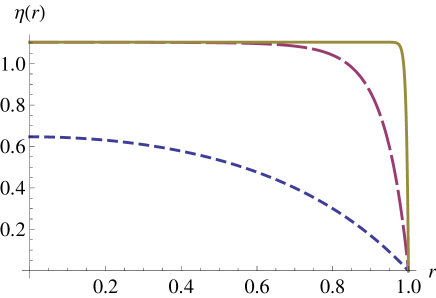
Figure 9: Radial profile of density add-on $\eta(r)=\rho(r)-\rho[1]$ inside a NRCO with size: $R=0.1$ (dash); $R=0.3$ (long dash); $R=1.0$ (solid). $R$ is measured in units $R_{-6}=10^{-6}R_{\odot}$.

The resulting density add-on at the center ($r=0$) of the NRCO, $\eta(0,R_{-6})$, depends on radius $R_{-6}$ as shown in Fig. 10. When NRCO’s radius is small, not much density add-on occurs. The center becomes denser, as the radius of the NRCO increases up to about $0.2\times R_{-6}$. Above $\sim 0.2\times R_{-6}$, the density add-on (and therefore the total density) at the center remains constant.

Therefore, the spherical configuration of the dense neutron matter composing the interior of the NRCO can indeed exist with the VdW-like equation of state with relativistic extension (produced by the system of equations (B4)-(B7)).

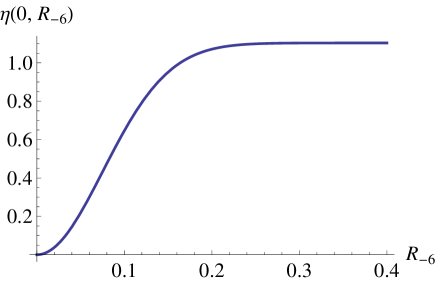
Figure 10: Density add-on $\eta(0,R_{-6})$ at the NRCO center ($r=0$) as a function of NRCO’s size ($R_{-6}$).

B.5 Mass-Radius dependence for the NRCO

The second boundary condition, Eq. (B17), permits finding the mass-radius relationship. Thus, from

$$m[r]=\frac{4\pi}{3}\rho[1]r^{3}+\mu[r]$$ (B29)

and boundary condition at $r=1$, it follows that

$$m[1]=\frac{4\pi}{3}\rho[1]+\mu[1]=\mu\frac{M}{(10^{-6}R_{-6})^{3}}.$$ (B30)

Here,

$$\mu[1]=(\frac{4\pi}{3}\rho[1]\alpha R_{-6}^{2})\times$$

$$\int_{0}^{1}ds\,s^{4}(1-\beta_{-6}R_{-6}^{2}s^{2})^{\kappa-1}F_{1}^{2}[\frac{3}{2},\kappa,\frac{5}{2},\beta_{-6}R_{-6}^{2}s^{2}].$$ (B31)

Solution of Eq. (B30) is

$$M(R_{-6})\simeq 9.237\times 10^{-5}R_{-6}^{3}+2.889\times 10^{-5}\alpha R_{-6}^{5}f[1,R_{-6}]).$$

(B32)

Here

$$f[1,R_{-6}]=$$

$$\int_{0}^{1}ds\,s^{4}(1-\beta_{-6}R_{-6}^{2}s^{2})^{\kappa-1}F_{1}^{2}[\frac{3}{2},\kappa,\frac{5}{2},\beta_{-6}R_{-6}^{2}s^{2}].$$

(B33)

This integral is calculated analytically and is expressed via a combination of hyper-geometrical functions $F_{1}^{2}[a,b,c,z]$. Numerical constants in Eqs. (B32) and (B33) are approximately $\alpha=1.95\times 10^{2}$, $\beta_{-6}=3.92\times 10^{-2}$, $\kappa=7.78\times 10^{2}$ and $\rho[1]=3.197$.

Fig. 11 plots NRCO’s mass as a function of radius, $M(R_{-6})$, for two cases – with and without the relativistic correction. Notably, the model has a limit, it occurs approximately when $M\sim 0.016$, $R_{-6}\sim 5$. Beyond that, at least for this particular set of chosen parameters $\xi=(T_{c}/m_{N}c^{2})=0.007$ and $T=0.1$, the model no longer applies.

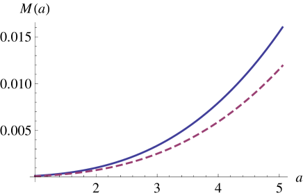
Figure 11: NRCO’s mass $M$ as a function of its size $R_{-6}$ for two cases: with relativistic correction (solid) and without (dash).

B.6 Summary of the results

We developed a model for the VdW-ike equation of state with a relativistic extension for a neutron-rich compact object (NRCO) composed of a highly dense neutron matter.

We presented a numerical solution for one set of the determining parameters, $\xi=(T_{c}/m_{N}c^{2})=0.007$ and $T=0.1$, which are within their commonly assumed ranges. The resulting model reveals the following characteristics of the NRCO:

Within the spherical NRCO, the density profile exhibits density increase (characterized in our model by the density ”add-on” $\eta$) toward the center of the NRCO.

For NRCOs with small radii ($R\leq 0.2\times 10^{-6}R_{\odot}$, in usual units), the overall density profile inside a NRCO exhibits a smooth maximum at the center (Fig. 9). The density add-on $\eta$ at any particular distance from the center increases as the NRCO size $R$ increases (Fig. 10).

For NRCOs with larger radii ($0.2\times 10^{-6}R_{\odot}<R\leq 5\times 10^{-6}R_{\odot}$, in usual units), the density distribution inside the NRCO is radially quasi-homogeneous, except for the narrow region near the edge where density gradient $\rho^{\prime}({\mathbf{r}}$) is negative and very steep. (See Fig. 9 and 10.)

Notably this model allows for the existence of NRCOs with smaller sizes than the traditionally assumed sizes of neutron stars. Indeed, the model is valid (for this set of $\xi$ and $T$) for NRCOs with sizes up to $R\leq 5\times 10^{-6}R_{\odot}$ (in usual units), i.e., $R<4\,km$.

Appendix C Decompression Model

The equations of state of a multi–body system of nucleons interacting via Skyrme potential (an analogy for the ”giant nucleus” of a NRCO) is presented in Fig. 12. (From Jaqaman et al. (1983).) The very steep part of the isotherms (on the left side) corresponds to the liquid phase. The gas phase is presented by the right parts of the isotherms where pressure is changing smoothly with increasing volume. Of special interest is the part of the diagram where the isotherms correspond to the negative compressibility, i.e. $(\partial P/\partial V)_{T}>0$. This is the so-called spinodal zone where the matter phase is unstable and can exist in both liquid and/or gas states. Within the spinodal zone lies a particularly unstable two-phased region (marked by the hatched line in Fig. 13), in which random density fluctuations lead to almost instantaneous collapse of the initially uniform system into a mixture of two phases – for nuclear matter, it is either liquid droplets surrounded by gas of neutrons, or homogeneous neutron liquid with neutron- gas bubbles.

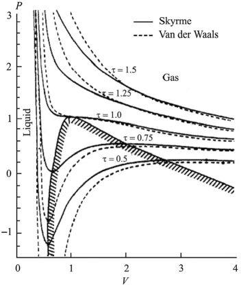
Figure 12: The equations of state $P(V)$ for a nuclear system interacting through a Skyrme potential and a Van der Waals compressible liquid-gas system (shown in relative units). (From Jaqaman et al. (1983).)

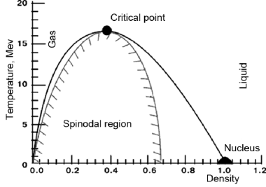
Figure 13: Theoretical $T(\rho)$ phase diagram for nuclear matter (adapted from (Karnaukhov, 2006)). The solid line is determined by condition $\partial p/\partial\rho=0$ and marks the phase transition zone. Density is expressed in units of $\rho_{nucleus}\simeq 2.85\times 10^{14}\,g/cm^{3}$. Temperature is expressed in $Mev$ units ($1\,Mev\simeq 10^{10}K$).

Figure 14: $T(\rho)$ phase diagram. Decompression path (solid line) of a localized pocket of the interior matter of the NRCO core. Depending on the initial state (solid dot) and the intensity of deceleration causing decompression, the state of the matter can shift into the two-phased region (area under dashed line) where the system cannot exist in the homogeneous state and forms nuclear fog – a two-phase mixture of nuclear liquid and nuclear vapor. The boundary of the two-phased zone is defined by condition $\partial p/\partial\rho=0$ (the zero speed of sound condition).

Critical temperature $T_{c}$ for the liquid-gas phase transition is a crucial characteristic of the nuclear equation of state. The nuclear equation of state (EoS), among other models, can be expressed (see Cherepanov, Karnaukhov (2009)) as follows:

$$p=a\rho-b\rho^{2}+c\rho^{3},$$ (C1)

where $a=k_{B}T_{c}(T/T_{c})$, $b=(k_{B}T_{c})/\rho_{c}$ and $c=2(k_{B}T_{c})/6\rho_{c}^{2}$. Coefficients $b$ and $c$ depend directly on the value of critical temperature $T_{c}$ and critical density $\rho_{c}$. This EoS is similar to Van der Waals equation suggested in 1875. For temperatures below the critical one, two distinct nuclear phases exist, and may coexist - liquid and gas. Above $T_{c}$, the two-phase equilibrium does not exist, only the nuclear vapor does.

It follows from Eq. (C1) that the square of sound speed in the nuclear matter, $s^{2}=\partial p/\partial\rho=a-2b\rho+3c\rho^{2}$, can be negative in some domain of densities, if temperature $T$ is small. However, the model (C1) needs to be modified for very large densities to not violate the principle of causality ($s<c_{light}$).

There exist many numerical estimates of $T_{c}$ for finite nuclei. But results depend strongly on the chosen model. For example, models using the Skyrme effective interaction and the thermal Hartree-Fock theory, employing the semi-classical nuclear model, based on the Seyler-Blanchard interaction, and several others, have been considered. Experimental measurements of the critical temperature of the nuclear liquid-gas phase transition produced a range: $5\,Mev<T_{c}<18\,Mev$ (Cherepanov, Karnaukhov (2009)).

The nuclear state where liquid and gas phases coexist, plays a crucial role in our collision scenario. As the NRCO decelerates and its interior matter pushes forward within the solid crust shell, the frontal part of the interior matter compresses, while the rear decompresses. The ($T,\rho$)-state of each individual localized ”increment” in the rear part can be visualized as ”sliding” down the decompression line on the $T(\rho)$-diagram (Fig. 14, dashed line) from its initial state to its final state depending on the intensity of deceleration causing decompression. If the ”sliding” path crosses the boundary of the two-phased region, the matter enters the zone of ”nuclear fog” where the gas and liquid phases coexist. Once in that state, individual sub-regions within the ”increments” may become significantly rarified to allow beta-decay and subsequent $r$-processes and fission. (See Section 3.5). The key question is thus whether the collision deceleration can produce meaningful density decompression to shift the state of the matter into the unstable zone.

C.1 Model of compression/decompression of the NRCO’s interior

Equations of motion of classical fluid in the frame moving with acceleration ${\mathbf{a}}(t)$, are

$$\partial_{t}\rho+\partial_{j}\rho u_{j}=0,$$

$$\rho\partial_{t}u_{i}+\rho u_{j}\partial_{j}u_{i}+\partial_{i}p=\rho g_{i}+\rho a_{i}(t),$$

$$\partial_{j}g_{j}=-4\pi G\rho.$$ (C2)

Eqs. (C2) must be completed by boundary conditions. Here $\rho$ is coordinate- and time-dependent density of the nuclear matter (not to be confused with definitions from prior sections), $p=p(\rho)$ is pressure within the nuclear fluid, ${\mathbf{u}}$ is collective fluid velocity, ${\mathbf{g}}$ is gravity acceleration generated by the distributed mass, ${\mathbf{a}}(t)$ is the externally-imposed deceleration (which does not depend on coordinates): $a_{i}(t)=-((c_{1})_{c}/\tau)\mu^{\prime}[((c_{1})_{c}\tau/L_{n})t]$. In the last expression, in contrast to Eqs. (C2), $t$ is the dimensionless time normalized on some $\tau$, prime signifies the derivative with respect to argument. For simplicity, the evolution process is assumed to be adiabatic (entropy per unit mass is constant).

By multiplying the first Eq. (C2) on $v_{i}$ and by combining the obtained equations, we obtain

$$-\partial_{t}^{2}\rho+\Delta(p+\rho v_{i}v_{j})=\partial_{i}(\rho g_{i})+a_{i}(t)\partial_{i}\rho,$$

$$\quad\quad\partial_{j}g_{j}=-4\pi G\rho$$ (C3)

In the equilibrium state, when the acceleration ${\mathbf{a}}(t)=0$ and the hydrodynamical velocity ${\mathbf{v}}=0$,

$$\Delta p_{s}=\partial_{i}(\rho g^{(s)}_{i}),\quad\partial_{j}g^{(s)}_{j}=-4\pi G\rho_{s}$$ (C4)

Letting $\rho_{1}=\rho-\rho_{s},\,p_{1}=p-p_{s}$, we obtain the nonlinear equations

$$-\partial_{t}^{2}\rho_{1}+\Delta(p_{1}+\rho v_{i}v_{j})=\partial_{i}(\rho_{s}g^{(1)}_{i})+$$

$$\partial_{i}(\rho_{1}g^{(s)}_{i})+\partial_{i}(\rho_{1}g^{(1)}_{i})+a_{i}(t)\partial_{i}\rho_{s}+a_{i}(t)\partial_{i}\rho_{1}\simeq$$

$$\partial_{i}(\rho_{s}g^{(1)}_{i})+\partial_{i}(\rho_{1}g^{(s)}_{i})+a_{i}(t)\partial_{i}\rho_{s},$$

$$\quad\quad\partial_{j}g^{(1)}_{j}=-4\pi G\rho_{1}$$ (C5)

By neglecting the secondary effects connected with self-gravity interaction and a hydrodynamical motion, $v^{2}\rightarrow 0$, we find the correlation between the leading terms in the equation

$$-\partial_{t}^{2}\rho_{1}+\Delta_{1}p_{1}\simeq a_{i}(t)\partial_{i}\rho_{s}.$$ (C6)

Switching to dimensionless variables $p\rightarrow p_{c}p$, $\rho\rightarrow\rho_{c}\rho$, $x_{k}\rightarrow R_{*}x_{k}$, we obtain

$$-\frac{\rho_{c}(c_{1})^{2}_{c}}{L_{n}^{2}}\partial_{t}^{2}\rho_{1}+\frac{p_{c}}{R^{2}_{*}}\Delta_{1}p_{1}\simeq\rho_{c}\frac{1}{R_{*}}[\partial_{x}\rho_{s}]\bigg{(}-\frac{(c_{1})^{2}_{c}}{L_{n}}\mu^{\prime}(t)\bigg{)}.$$

Prime signifies the derivative with respect to argument. Thus,

$$\epsilon\beta\partial_{t}^{2}\rho_{1}+\Delta_{1}p_{1}\simeq\beta\,\rho_{s}^{\prime}\,\mu^{\prime}(t)\,\frac{x}{\sqrt{x^{2}+{\mathbf{x}}_{\perp}^{2}}}.$$

Here, we introduced the small dimensionless parameters $\epsilon=R_{*}/L_{n}\ll 1$ and $\beta=({R_{*}}/{L_{n}})({(c_{1})_{c}}/{c})^{2}({\rho_{c}c^{2}}/{p_{c}})$. In leading approximation with respect to $\epsilon$, Eq. (C.1) becomes

$$(\Delta_{\perp}+\partial_{x}^{2})p_{1}\simeq\beta\mu^{\prime}(t)[\rho_{s}]^{\prime}\frac{x}{\sqrt{x^{2}+{\mathbf{x}}_{\perp}^{2}}}.$$ (C7)

The solution of Eq. (C7) is expressed via the Green function of the problem $(\Delta_{\perp}+\partial_{x}^{2})G(|{\mathbf{x}}-{\mathbf{z}}|)=\delta^{(3)}({\mathbf{x}}-{\mathbf{z}})$ with zero boundary condition for pressure $p_{1}=0$, and the for boundary condition $G(|{\mathbf{x}}-{\mathbf{s}}|)=0$ for the Green function on the surface of container $|{\mathbf{s}}|=1$:

$$p_{1}\simeq\beta\mu^{\prime}(t)\int d{\mathbf{r}}_{1\perp}dx_{1}\,G(|{\mathbf{x}}-{\mathbf{x}}_{1}|)\rho_{s}^{\prime}(|{\mathbf{x}}_{1}|)\frac{x_{1}}{\sqrt{x_{1}^{2}+{\mathbf{r}}_{1\perp}^{2}}}.\;$$

(C8)

Eq. (C8) shows that the magnitude of $p_{1}$ is not identically zero. It can be positive or negative, and depends strongly on the behavior of $\rho_{s}$ inside of the NRCO, especially near the gas-liquid phase transition boundary. Since $p_{1}\sim\mu^{\prime}$ (Eq. C8) and $p_{1}=p(\rho_{s}+\rho_{1})-p(\rho_{s})\simeq s^{2}(\rho_{s})\rho_{1}$, it means that when $s^{2}\rightarrow 0,$ the magnitude of density perturbation $\rho_{1}$ can reach very large (positive or negative) values.

This means that when the NRCO deceleration $\mu^{\prime}$ is sufficiently strong, significant decompression may indeed occur.

Appendix D Model describing deceleration of a NRCO due to accretion of surrounding nebula particles

As mentioned, when a colliding object, like the NRCO, penetrates a target, multiple effects contribute to dissipation of its kinetic energy and cause deceleration. Depending on the properties of the target, such effects as hydrodynamical drag, Cherenkov–like radiation of various waves related to collective motions generated within the target, gravitational accretion of target particles onto the NRCO, or distortion of the magnetic fields, may actually play meaningful roles. Here, we focus only on the effect of accretion of the gaseous target particles onto the gravitationally powerful NRCO.

Accretion onto a supersonically moving star has been studied both theoretically and numerically. (See review by Edgar, Clarke (2004).) The early works of Hoyle, Lyttleton (1939) and Bondi (1952) considered accretion by a star moving at a steady speed through an infinite gas nebula. Later, the problem was applied to accretion of particles from interstellar medium, a stellar wind, or a common envelope (where two stellar cores become embedded in a large gas envelope formed when one member of the binary system swells) (Petterson, 1978; Taam, Sandquist, 2000; Dokuchaev, 1964; Bonnell I. A. et al., 2001; Edgar, Clarke, 2004; Ruffert, 1994; Bisnovatyi-Kogan, Pogorelov, 1997; Pogorelov et al., 2000; Toropina, Romanova & Lovelace, 2012). Accretion onto a neutron star from the supernova ejecta has also been extensively researched – for a radially-outflowing ejecta (Colgate, 1971; Zeldovich, Ivanova & Nadezhin, 1972), for an in-falling ejecta (Chevalier, 1989; Colpi, Shapiro & Wasserman, 1996) and even when a star is moving at a high speed across the supernova ejecta (Zhang, Lu & Zhao, 2007).

The equation of motion for a body of variable mass follows from the law of conservation of linear momentum of the entire system composed of the object and the surrounding mass captured by the object (Meshcherskii, 1887). Thus, when a neutron star enters a dense gaseous ”cloud”, and surrounding nebula particles accrete onto the gravitationally powerful star, the motion of the star will be described by $d(M_{*}{\mathbf{V}})-{\mathbf{v}}\,dM_{*}=\delta{\mathbf{I}}.$ Here $M_{*}(t)$ and $\mathbf{V}(t)$ denote, respectively, the mass and velocity of the moving star in a inertial frame at instance $t$, ${\mathbf{v}(t)}$ is the velocity in the same frame of the accreting nebula particles which constituent the composing mass $dM_{*}$), and $d(...)$ denotes change of quantities over the interval of time $dt$. Quantity $\delta{\mathbf{I}}=M_{*}{\mathbf{a}}\,dt$ (where ${\mathbf{a}(t)}$ is acceleration) is the impulse of an external force ${\mathbf{F}}=M_{*}\,{\mathbf{a}}$. Then it follows:

$$d{\mathbf{V}}+({\mathbf{V}}-{\mathbf{v}})\,\frac{dM_{*}}{M_{*}}={\mathbf{a}}dt.$$ (D1)

Expression (D1) must be statistically averaged with respect to all possible values of velocities of the accreting particles for the given $dM_{*}$. After the averaging, the velocity ${\mathbf{v}}$ of accreting fragment $dM_{*}$ in Eq. (D1) which contains a large number of accreting particles, is replaced by averaged $\overline{{\mathbf{v}}}$.

To derive the expression for $\overline{{\mathbf{v}}}$, we assume that the surrounding gas is composed purely of ionized hydrogen–degenerated electron–proton plasma. Since $m_{p}\gg m_{e}$, only the proton component is significant for the star mass change. We assume spherical symmetry of the velocity distribution of the gas particles, so that distribution function $f({\mathbf{v}})=f(v)$ is a function of velocity module. The probability that any gas particle occupies element $dw=dv_{x}dv_{y}dv_{z}$ in the space of velocities is proportional to $dw\,f(v).$ The probability of the star to capture the gas particle with velocity ${\mathbf{v}}$ is proportional to the cross–section of interaction, i.e. to the product of the module of relative velocity of the particle with respect to the star ($|{\mathbf{v}}-{\mathbf{V}}|$) and $dw\,f(v)$. Thus, the average velocity is

$$\overline{{\mathbf{v}}}=\frac{\int dw\,{\mathbf{v}}\,|{\mathbf{v}}-{\mathbf{V}}|\,f(v)}{\int dw\,|{\mathbf{v}}-{\mathbf{V}}|\,f(v)}$$ (D2)

Due to the axial symmetry of the problem, $\overline{{\mathbf{v}}}$ is co-linear with ${\mathbf{V}}.$ In the spherical coordinate system with $dw=$ $2\pi d\theta\,\sin\theta\,dv\,v^{2}$ where $\theta$ is the angle between ${\mathbf{v}}$ and ${\mathbf{V}},$

$$\overline{v}=$$

$$\frac{2\pi\int_{0}^{\infty}\int_{0}^{\pi}dv\,v^{2}\,d\theta\,\sin\theta\,f(v)v\,\cos\theta\,\sqrt{v^{2}+V^{2}-2vV\cos\theta}}{2\pi\int_{0}^{\infty}\int_{0}^{\pi}dv\,v^{2}\,d\theta\,\sin\theta\,f(v)\,\sqrt{v^{2}+V^{2}-2vV\cos\theta}},$$

which, after integrating with respect to angle $\theta,$ produces the following expression:

$$\overline{v}=$$

$$\frac{\int_{0}^{V}dv\,v^{3}f(v)[\frac{2}{3}v-\frac{2}{15}\frac{v^{3}}{V^{2}}]+\int_{V}^{\infty}dv\,v^{3}f(v)[\frac{2}{3}V-\frac{2}{15}\frac{V^{3}}{v^{2}}]}{\int_{0}^{V}dv\,v^{2}f(v)[2V+\frac{2}{3}\frac{v^{2}}{V}]+\int_{V}^{\infty}dv\,v^{2}f(v)[2v+\frac{2}{3}\frac{V^{3}}{v^{2}}]}.$$

For the distribution with respect to velocities of fully degenerated non–relativistic Fermi gas (Fermi, 1929, 1965, 1946), $f(v)\sim H(v_{F}-v)$, where $v_{F}$ is the local Fermi boundary velocity of the nebula particles and $H[\xi]$ is the Heaviside step function.

When temperatures of proton– and electron–components of the nebula are of the same order, parameter $v_{F}=(6\pi^{2}/2)^{1/3}\hbar(\rho/m_{p})^{1/3}/m_{p}$ is of the same order as the speed of sound $c_{n}$ in the nebula, and we can write it as $v_{F}=\sqrt{3}\,c\,c_{1}\rho^{1/3}$ where numerical coefficient $c_{1}$ combines most of the constants, and $c$ is the speed of light. This allows us to simplify our subsequent analysis by introducing dimensionless velocity $\mu=V/v_{F}$ and expressing $\overline{v}$ as

$$\overline{v}=-v_{F}\frac{[-24\mu^{7}+\alpha_{1}(\mu)H[-1+\mu]+\alpha_{2}(\mu)H[1-\mu]}{\beta_{1}(\mu)H[-1+\mu]+\beta_{2}(\mu)[1-\mu])}$$

$$\equiv v_{F}\Phi(\mu).\quad$$ (D3)

Here $\alpha_{1}(\mu)=4(1-7\mu^{2}+6\mu^{7})$, $\alpha_{2}(\mu)=7\mu^{3}(-5+2\mu^{2}+3\mu^{4})$, $\beta_{1}(\mu)=7\mu(-24\mu^{5}+4(-1-5\mu^{2}+6\mu^{5})$ and $\beta_{2}(\mu)=5\mu(-3-2\mu^{2}+5\mu^{4})$ (For small $\mu$, $\Phi(\mu)\simeq-\frac{1}{3}\mu+\frac{16}{45}\mu^{3}$; for large $\mu$, $\Phi(\mu)\simeq-\frac{1}{5\mu}+\frac{12}{175\mu^{3}}$). Then Eq. (D1) (without the term $\mathbf{a}$) takes form suitable for our analysis:

$$\frac{d{\mathbf{\mu}}}{dt}=(-\frac{\dot{M}_{*}}{M_{*}})(1-\frac{1}{\mu}\Phi(\mu)){\mathbf{\mu}}$$ (D4)

In a simplified interpolating form, this expression for $\overline{v}$ can be parameterized as

$$\overline{v}=v_{F}(-\frac{86.25\mu}{3\times 86.25+5\times 96.59\mu^{2}})\,,$$ (D5)

which is valid for cases of both small and large of the parameter $\mu=v/v_{F}$.

Next we express star mass $M_{*}(t)$ in terms of (constant) $M_{*}$ (which from this point on will be labeling the initial mass of the star) and the normalized variable $m(t)$, so that $M_{*}(t)=M_{*}m(t)$. Nebula density will be denoted $\rho({\mathbf{r}})=\rho_{c}\,\rho(t)$ where ${\mathbf{r}}$ is the radius vector from the center of the nebula, $\rho_{c}$ is the nebula density in its center. We introduce $(c_{1})_{c}$, sound speed in the nebula center. Note that $v_{F}=\sqrt{3}(c_{1})_{c}\rho^{1/3}(t)$. We also will transition from old $\mu=V/v_{F}$ to new $\mu=V/(c_{1})_{c}$ (which leads to recalculation of coefficients in front of $\mu$). After all these manipulations, we then obtain the dimensionless equation of motion for the compact star:

$$\dot{\mu}(t)+$$

$$\bigg{(}1+\frac{86.25\rho^{2/3}(t)}{160.99\mu^{2}(t)+258.75\rho^{2/3}(t)}\bigg{)}\mu(t)\frac{\dot{m}(t)}{m(t)}=0.$$ (D6)

Here $\tau$ is the time–scale and all time derivatives are dimensionless. Coefficient $(c_{1})_{c}=c(1.83/c\sqrt{3})\times 10^{3}(\rho_{c}/\rho_{\odot})=3.524\times 10^{-6}\rho^{1/3}\,c$, where $c$ is the speed of light, (constant) $\rho_{c}$ is the density of the target nebula at its center, and we again will express nebula density in terms of a constant, $\rho_{c}$, and a new normalized variable $\rho(t)$, so that $\rho=\rho_{c}\rho(t)$ or $(\rho_{c}/\rho_{\odot})\rho_{\odot}\rho(t)$, if expressed in the units of the average density of the Sun $\rho_{\odot}=1.384\times 10^{3}\,kg/m^{3}$. Also, $R=R_{*}/R_{\odot}$ and $M=M_{*}/M_{\odot}$. Going forward, we will label $\rho\equiv\rho_{c}/\rho_{\odot}$ and $\rho(t)$ will be the normalized dimensionless variable.

Eq. (D) describing the evolution of $\mu(t)$ contains two more time-dependent variables, $m(t)$ and $\rho(t)$. Thus we need to develop evolution equations for each of them to complete our system of equations.

As mentioned, nebula density is a function of coordinates. The most general mono–parametric expression for it is $\rho({\mathbf{r}})=\rho_{c}F({\mathbf{r}}/L_{n})$. It implies that maximum of density $\rho_{c}$ is located at the center ($r=0$) and density decays away from the center over the characteristic scale $L_{n}$. Nebula density at the point of the compact star location is then expressed as $\rho({\mathbf{r}}(t)=\rho_{c}F({\mathbf{r}}(t)/L_{n})$, where ${\mathbf{r}}(t)$ is radius vector to location of the star, $F(\xi)$ is some function of radius. To dimensionalize the equation below, we write ${\mathbf{r}}(t)=L_{n}{\mathbf{s}}(t)$. Because derivative $d{\mathbf{r}}/dt={\mathbf{V}}(t)$, then $(L_{n}/(c_{1})_{c}\tau)\,d{\mathbf{s}}/dt={\mathbf{V}}(t)/(c_{1})_{c}\equiv{\mathbf{\mu}}$. If time-scale $\tau$ is chosen as $\tau=L_{n}/(c_{1})_{c}$, the second equation of the system connecting variables $\mu(t)$ and $s(t)$ – the implicit form of the nebula density – is then

$$\dot{s}(t)-\mu(t)=0.\quad\quad$$ (D7)

To derive expression for the evolution of star mass $m(t)$, we employ expression for $\dot{M}_{*}$ due to accretion proposed by Bondi (Bondi, 1952):

$$\dot{M}_{*}\equiv\pi R^{2}_{ac}\,\rho_{\infty}\,V=4\pi\alpha(GM_{*})^{2}{\rho_{\infty}}{(V^{2}+c_{\infty}^{2})^{-3/2}}$$ (D8)

(see also, Shapiro, Teukolsky (1983), p. 420). Here, $\rho_{\infty}$ is the medium density at large distance from accreting body, $V$ is the velocity of the accreting body, $c_{\infty}$ is the sound speed in the nebula at large distance from the accreting body, coefficient $\alpha$ is of the order of unity.

In terms of dimensionless quantities $m(t),\,\rho(t)$ with time scale $\tau=L_{n}/(c_{1})_{c})$, we obtain for the nebula composed from the degenerated Fermi–gas

$$\frac{dm(t)}{dt}=(4\pi\alpha G^{2}\rho_{\odot}\frac{M_{\odot}R_{\odot}}{(c_{1})_{c}^{4}})ML\rho\times$$

$$\frac{m^{2}(t)\rho(t)}{(\mu^{2}(t)+\rho^{2/3}(t))^{3/2}}.$$ (D9)

Here, $M=M_{*}/M_{\odot}$ is the initial compact star mass measured in units of the Sun’s mass ($M_{\odot}=2\times 10^{30}\,kg$), $L=L_{n}/R_{\odot}$ is the characteristic nebula size (in units of the Sun’s radius, $R_{\odot}=7\times 10^{8}\,m$), $\rho=\rho_{c}/\rho_{\odot}$ is the density of the nebula in its center (in units of the average density of the Sun, $\rho_{\odot}=1.38\,g/cm^{3}$). Dimensionless accretion parameter $k_{A}=4\pi\alpha G^{2}\rho_{\odot}{M_{\odot}R_{\odot}}/{(c_{1})_{c}^{4}}$ is composed of universal constants, and can be is expressed in terms of the escape velocity for Sun, $V_{\odot}=\sqrt{2GM_{\odot}/R_{\odot}}=6.16\times 10^{2}\,km/s$, and the speed of light, $c=2.99\times 10^{8}\,m/s$, as

$$k_{A}=\frac{3\alpha}{4}(\frac{V_{\odot}}{(c_{1})_{c}})^{4}=8.633\times 10^{10}\alpha\rho^{-4/3}$$ (D10)

Finally,

$$\frac{dm(t)}{dt}=k_{A}ML\rho\frac{m^{2}(t)\rho(t)}{(\mu^{2}(t)+\rho^{2/3}(t))^{3/2}}$$ (D11)

where $\rho(t)$ is the normalized dimensionless density of the nebula.

Eqs. (D), (D7) and (D11) complete the system of equations necessary to study the problem, subject to some assumption about the shape of the spacial distribution profile of nebula density $\rho(\,s(t)\,)$. In our model we assume that $\rho(t)=\exp(-s^{\nu}(t))$ and that $\nu=2$.

References

- Abramovitz & Stegun (1964) Abramovitz M., Stegun I. A., 1964, Handbook of Mathematical Functions, eds., U. S. Govt. Printing Office, Washington D. C.
- Abt (1983) Abt H., 1983, Ann. Rev. Astron. Astrophys, 21, 343
- Adams (2010) Adams F., 2010, Ann. Rev. Astron. Astrophys., 48, 47; preprint(arXiv:1001.5444. [astro-ph.SR])
- Batygin et al. (2011) Batygin K., Brown M. E., Betts H., 2011, preprint(arXiv:1111.3682v1 [astro-ph.EP])
- Baym (1991) Baym G., 1991, in Ventura J., Pines D., eds., Neutron Stars: Theory and Observation, Kluwer
- Beck, Giles (2005) Beck J. G., Giles P., 2005, ApJ, 621, L153
- Beer et al. (2004) Beer at al., 2004, MNRAS, 354, 763
- Bertsch et al. (1983) Bertsch G. F. et al., 1986, Phys. Lett. B, 126, 9
- Beskin (1999) Beskin V. S., 1999, Phys. Usp., 42, 1071 [Usp. Fiz. Nauk 169, 1169 (1999)]
- Bisnovatyi-Kogan, Pogorelov (1997) Bisnovatyi-Kogan G. S., Pogorelov N. V., 1997, Astronomical and Astrophysical Transactions, 12, 263–280.
- Bodenheimer (1995) Bodenheimer P., 1995, ARA&A, 33, 199
- Bondi (1952) Bondi H., 1952, MNRAS, 112, 195
- Bonnell I. A. et al. (2001) Bonnell I. A., Bate M. R., Clarke C. J., Pringle J. E., 2001, MNRAS, 323, 785
- Borderie (2002) Borderie B, 2002, J. Phys. G: Nuclear Part. Phys., 28, R217
- Borderie Rivet (2008) Borderie B., Rivet M. F., 2008, Progress in Particle and Nuclear Physics, 61, 551–601
- Boss (1995, 2005) (a) Boss A. P., 1995, ApJ, 439, 224; (b) Boss A. P., Durisen R. H., 2005, ApJ, 621, L137
- Boss Foster (1998) Boss A. P., Foster P. N., 1998, ApJ, 494, L103
- Boss, Keiser (2012) Boss A. P., Keiser S. A., 2012, ApJ Lett., 756, L9
- Cameron, Truran (1977) Cameron A. G. W., Truran J. W, 1977, Icarus, 30, 447
- Cameron et al. (1995) Cameron A. G. W., Hoeflich P., Myers P. C., Clayton D. D., 1995, ApJ, 447, L53
- Chaussidon et al. (2001) Chaussidon M., Robert F., McKeegan K. D., Krot A. N., 2001, Lunar Planet. Sci. Conf., 32, 1862
- Chaussidon, Robert, McKeegan (2002) Chaussidon M., Robert F., McKeegan K. D., 2002, Lunar Planet. Sci. Conf., 33, 1563
- Cherepanov, Karnaukhov (2009) Cherepanov E. A., Karnaukhov V. A., 2009, Communication of the Joint Institute for Nuclear Research, Dubna, preprint(http://www1.jinr.ru/Preprints/2009/ 004(E7-2009-4).pdf)
- Chevalier (1989) Chevalier R. A., 1989, ApJ, 346, 847
- Chodos et al. (1974) Chodos A., Jaffe R. I., Jonson K., Thorn C. B., Weisskopf V. F., 1974, New extended model of hadrons, Phys. Rev. D, 9, 3471
- Chugunov, Horowitz (2010) Chugunov A. I., Horowitz C. J., 2010, MNRAS Letters, 407, 54
- Colgate (1971) Colgate S. A., 1971, ApJ, 63, 221
- Colpi, Shapiro & Wasserman (1996) Colpi M., Shapiro S. L., Wasserman I., 1996, ApJ, 470, 1075
- Csernai (1986) Csernai L.P. et al., 1986, Phys. Rep., 131, 223
- Diener et al. (1997) Diener P. et al, 1997, ApJ, 479, 164
- Dokuchaev (1964) Dokuchaev V. P., 1964, Soviet Astronomy, 8, 23
- Duquennoy, Mayor (1991) Duquennoy A., Mayor M., 1991, A&A, 248, 485
- Edgar, Clarke (2004) Edgar R., Clarke C., 2004, MNRAS, 349, 678
- Fermi (1929, 1965) Fermi E., a) Rend. Lincei, 9, 984 (1929); b) Fermi, E., 1972, in Pontecorvo B., Pokrovskii V., eds, Scientific Works of E. Fermi, Nauka, Moscow, p. 588 [in Russian ]; see also Collected Papers of Enrico Fermi, 1965, Univ. Chicago Press, Chicago
- Fermi (1946) Fermi E., 1946, A course in Neutron Physics (document LADC-225, 5 February 1946), in Collected Papers of Enrico Fermi, Univ. Chicago Press, Chicago
- Ford et al. (2001) Ford F. B., Havlickova M., Rasio F. A., 2001, Icarus, 150, 303
- Fortov (2009) Fortov V., 2009, Physics - Uspekhi, 52 (6), 615
- Freiburghaus et al. (1999) Freiburghaus C., Rosswog S., Thielemann F.-K., 1999, ApJ, 525, L121
- Fryer et al. (1996) Fryer C. I. et al., 1996, ApJ, 460, 801
- Gaidos et al. (2009) Gaidos E., Krot A. N., Williams J. P., Raymond S.N., 2009, ApJ, 696, 1854–1863.
- Glendenning (2000) Glendenning N. K., 2000, Compact Stars: Nuclear Physics, Particle Physics, and General Relativity, 2nd ed, Springer, NY
- Goodman et al. (1984) Goodman A.L., Kapusta J. I., Mekjian A. Z., 1984, Phys. Rev. C, 30, 851
- Goswami, Marhas, Sahijpal (2001) Goswami A. N., Marhas K. K., Sahijpal S., 2001, ApJ, 549, 1151
- Goswami, Vanhala (2000) Goswami J. N., Vanhala H. A. T., 2000, in Mannings A. P., Boss S.S., Russell, eds, Protostars and Planets IV., Univ. Arizona Press, Tucson, pp. 963–994
- Gounelle et al. (2001) Gounelle M., et al., 2001, ApJ, 548, 1051
- Gritschneder et al. (2012) Gritschneder et al., 2012, ApJ, 745, 22–34
- Haensel, Potekhin & Yakovlev (2007) Haensel P., Potekhin A. Y., Yakovlev D. G., eds, 2007, Neutron Stars 1: Equation of State and Structure, 326, Astrophysics and Space Science Library
- Heiselberg et al. (1988) Heiselberg H. et al., 1988, Phys. Rev. Lett., 61, 818
- Hogg et al. (1991) Hogg D.W., Quinlan G.D., Tremaine S., 1991, AJ, 101, 227
- Horowitz, Kadau (2009) Horowitz C. J., Kadau K., 2009, Phys. Rev. Lett., 102, 191102
- Hoyle, Lyttleton (1939) Hoyle F., Lyttleton R. A., 1939, Proc. Cambridge Philos. Soc., 36, 323
- Jaqaman et al. (1983) Jaqaman H., Mekjian A. Z., Zamick L., 1983, Phys. Rev., 27, 2782
- Jaqaman, et al. (1984) Jaqaman H.R. et al., 1984, Phys. Rev. C, 29, 2067
- Karnaukhov (2006) Karnaukhov V. A., 2006, Phys. elem. particles, 37, 2, 313
- Karnaukhov et al. (2011) Karnaukhov V. A. et al., 2011, Properties of Hot Nuclei Produced in Relativistic Collisions; preprint(http://fias.uni-frankfurt.de/ historical/nufra2011/talks/Karna-NUFRA.pdf)
- Kenyon, Bromley (2004) Kenyon S. J., Bromley B. C., 2004, Nature, 432, 598
- Kley (2000) (a) Kley W. , 2000, MNRAS, 313, L47; (b) Kley W., Peitz J., Bryden G., 2004, A&A, 414, 735
- Kraus et al. (2011) Kraus A. L., Ireland M. J., Martinache F., Hillenbrand L.A., 2011, AJ, 731, 8
- Kutschera (1998) Kutschera M., 1998, Acta Physica Polonica B, 29 (1-2), 25
- Landau, Lifshitz (1969) Landau L. D., Lifshitz E. M., 1969, Statistical Physics, 2nd ed., Addison-Wesley, Reading, Massachusetts, sec. 66
- Landau, Lifshitz (1975) Landau L. D., Lifshitz E. M., 1975, The Classical Theory of Fields, 4th rev. ed., Pergamon, Elmsford, NY, sec. 64
- Landau, Lifshitz (1987) Landau L. D., Lifshitz E. M., 1987, Fluid Mechanics, Elsevier, 2nd edition
- Lattimer, Schramm (1976) Lattimer J. M., Schramm D.N., 1976, ApJ, 210, 549
- Lattimer, Swesty (1991) Lattimer J. M., Swesty D., 1991, Nucl. Phys. A, 535, 331
- Lee et al. (1998) Lee T. et al., 1998, ApJ, 506, 898
- Leya et al. (2003) Leya I., Halliday A. N., Wieler R., AJ, 2003, 594, 605
- Looney et al. (2006) Looney L. W., Tobin J. J., Fields B. F., 2006, ApJ, 652, 1755
- Lopez et al. (1989) Lopez J. et al., 1989, Phys. Lett. B, 219, 215
- Masset, Snellgrove (2001) Masset F. S., Snellgrove M. D., 2001, MNRAS, 320, L55
- Meshcherskii (1887) Meshcherskii I. V., 1897, PhD thesis, Univ. S-Peterburg
- Muller et al. (1995) Muller H. et al., 1995, Phys. Rev. C, 52, 2072
- Nagamia (1988) Nagamia S., 1988, Nucleus-Nucleus III,
- Nesvorny (2011) Nesvorny D., 2011, ApJ Letters, 742, L22
- Nomoto et al. (2006) Nomoto K., Tominaga N., Umeda H., Kobayashi C., Maeda K., 2006, Nucl.Phys. A, 777, 424–458
- Pavlov, Kharin (1990) Pavlov V. I., Kharin O. A., 1990, Sov. Phys. - JETP, 71 (2), 211
- Pavlova (1992) Pavlova E., 1992, Herald of Moscow State University, Physics–Astronomy, 33 (2), 97
- Pethick, Ravenhall (1991) Pethick, Ravenhall, 1991, in Ventura J., Pines D., eds, Neutron Stars: Theory and Observation, Kluwer
- Petterson (1978) Petterson J. A., 1978, ApJ, 224, 625
- Pogorelov et al. (2000) Pogorelov N. et al., 2000, Astrophysics and Space Science, 274, Issue 1/2, 115–122
- Potekhin (2010) Potekhin A. Y., 2010, Physics–Uspekhi, 53 (12), 1235
- Rauscher et al. (2013) Rauscher T. et al., 2013, Rep. Prog. Phys., 76, 066201
- Rohlf (1994) Rohlf J. W., 1994, Modern Physics from A to Z, Wiley
- Ruffert (1994) Ruffert M., 1994, ApJ, 427, 342
- Sauer et al. (1976) Sauer G., Chandra H., Mosel U., 1976, Nucl. Phys. A, 264, 221
- Silva et al. (2004) Silva J. D. et al., 2004, Phys. Rev. C, 69, 024606
- Schiller et al. (2012) Schiller M., Paton C., Bizzarro M., 2012, 75th Annual Meeting of the Meteoritical Society, held August 12-17, 2012 in Cairns, Australia. Published in Meteoritics and Planetary Science Supplement, id.5211
- Shapiro, Teukolsky (1983) Shapiro S. L., Teukolsky S. A., 1983, Black Holes, White Dwarfs and Neutron Stars, John Wiley & Sons Inc., NY
- Sigurdsson et al. (2003) Sigurdsson S., Richer H. B., Hansen B. M., Stairs I. H., Thorsett S. E., 2003, 193
- Taam, Sandquist (2000) Taam R. E., Sandquist E. L., 2000, ARA&A, 38, 113
- Taras et al. (2004) Taras S. et al., 2004, Phys. Rev. C, 69, 014602
- Thommes, Duncan & Levison (2003) Thommes E. W., Duncan M. J., Levison H. F., 2003, Icarus, 161, 431
- Toropina, Romanova & Lovelace (2012) Toropina O. D., Romanova M. M., Lovelace R. V. E., 2012, MNRAS, 420, 810
- Tremaine (1990) Tremaine S., 1990, in Lynden-Bell D. and Gilmore G., eds, Baryonic Dark Matter, NASA ASI Ser., C 306, 37
- Tsang et al. (2011) Tsang et al., 2011, preprint(arXiv:1110.0467 [astro-ph.HE])
- Tsiganis et al. (2005) Tsiganis et al., 2005, Nature, 435, 459
- Yakovlev, Levenfish & Shibanov (1999) Yakovlev D. G., Levenfish K. P., Shibanov Yu. A., 1999, Phys. Usp., 42, 737 [Usp. Fiz. Nauk 169, 825 (1999)]
- Wadhwa et al. (2007) Wadhwa M. et al., 2007, in Reipurth B., Jewitt D., Keil K., eds, Protostars and Planets, 835–848, Univ. Arizona Press, Tucson
- Wapstra (1958) Wapstra A. H., 1958, Atomic Masses of Nuclides, Springer
- Wasserburg et al. (2006) Wasserburg G. J., Busso M., Gallino R., Nollett K.M., 2006, Nuclear Phys. A, 777, 5
- Woosley et al. (2002) Woosley S.E., Heger A., Weaver T. A., 2002, Rev. Mod. Phys, 74, 1015
- Zhang (1996) Zhang Feng Shou, 1996, Z. Phys. A, 356, 163
- Zhang, Lu & Zhao (2007) Zhang X., Lu Y., Zhao Y.H., 2007, Chin. J. Astron. Astrophys (ChJAA), 7, 91
- Zeldovich, Ivanova & Nadezhin (1972) Zeldovich Ya. B., Ivanova L. N., Nadezhin D. K., 1972, Soviet Ast.-AJ, 16, 209
- Zel’dovich, Novikov (1996) Zel’dovich Ya. B., Novikov I. D., 1996, Relativistic Astrophysics, Vol. 1: Stars and Relativity, Dover Publications, Mineola, NY