Fluctuations and information filtering in coupled populations of spiking neurons with adaptation

Abstract

Finite-sized populations of spiking elements are fundamental to brain function, but also used in many areas of physics. Here we present a theory of the dynamics of finite-sized populations of spiking units, based on a quasi-renewal description of neurons with adaptation. We derive an integral equation with colored noise that governs the stochastic dynamics of the population activity in response to time-dependent stimulation and calculate the spectral density in the asynchronous state. We show that systems of coupled populations with adaptation can generate a frequency band in which sensory information is preferentially encoded. The theory is applicable to fully as well as randomly connected networks, and to leaky integrate-and-fire as well as to generalized spiking neurons with adaptation on multiple time scales.

I Introduction

Multi-scale modeling of complex systems has led to important advances in fields as diverse as complex fluid dynamics, chemical biology, soft matter physics, meteorology, computer science, and neuroscience (Klein and Shinoda, 2008; Ayton et al., 2007; Peter and Kremer, 2009; Pielke, 2002; Benaïm and Le Boudec, 2008; Gerstner et al., 2012). In these approaches, mathematical methods such as mean-field theories and coarse-graining provide the basis to link properties of microscopic elements to macroscopic variables. In many cases, macroscopic variables fluctuate due to a finite number of microscopic elements. For instance, in the brain, neurons can be grouped into populations of $50$ to $1000$ neurons (Lefort et al., 2009) with similar properties (Hubel and Wiesel, 1962; Mensi et al., 2012). Fluctuations of the global activity of such populations are not captured in classical mean-field theories (Brunel and Hakim, 1999; Gerstner, 2000), which assume infinite system size. Here we put forward a theory for the fluctuating macroscopic activity in networks of pulse-coupled elements occurring in neuronal networks (Pillow et al., 2008), queuing theory (Frost and Melamed, 1994) and synchronizing fireflies (Mirollo and Strogatz, 1990).

Finite-size effects in networks of spiking elements have been approached by different methods, including extensions of the Fokker-Planck equation for neuronal membrane potentials (Brunel and Hakim, 1999; Mattia and Del Giudice, 2002), stochastic field theory (Buice and Chow, 2013), moment expansions in networks of generalized linear models (GLM) (Toyoizumi et al., 2009), modified Hawkes processes (Hawkes, 1971; Pernice et al., 2012; Helias et al., 2013), simplified Markov neuron models (Soula and Chow, 2007; Buice and Cowan, 2007; Bressloff, 2009; Benayoun et al., 2010; Touboul and Ermentrout, 2011; Dumont et al., 2014; Lagzi and Rotter, 2014) and the use of a linear response formalism for spike trains perturbed by finite-size fluctuations (Lindner et al., 2005; Ávila Åkerberg and Chacron, 2009; Trousdale et al., 2012). These studies lack, however, slow cellular feedback mechanisms mediating adaptation.

Adaptation characterized by a reduced response of a neuron to slow compared to fast inputs is a wide-spread phenomenon in the brain and has important implications for signal processing (Benda and Herz, 2003; Lundstrom et al., 2008; Pozzorini et al., 2013; Farkhooi et al., 2013) and the spontaneous activity of single neurons (Prescott and Sejnowski, 2008; Schwalger, 2013; Schwalger and Lindner, 2013). On the population level, adaptation has been recently analyzed using a quasi-renewal (QR) theory (Naud and Gerstner, 2012). The QR framework uses tools of renewal point process theory (Cox and Isham, 1980) to treat neurons with arbitrary refractoriness. In particular, the dynamics of the population activity is determined by an integral equation (Wilson and Cowan, 1972; Gerstner, 2000; Deger et al., 2010). These studies, however, have assumed an infinitely large population.

Here we present a theory for the interaction of finite-sized populations of adapting neurons. The theory is valid for the broad class of neuron models that can be approximated by a QR point process. This includes integrate-and-fire (IF) as well as GLM neurons, for which parameters can be reliably extracted from experimental data (Pillow et al., 2008; Truccolo et al., 2010; Mensi et al., 2012).

Based on this theory we analyze information filtering (noise shaping) in neuronal populations. We show that in a single population no noise shaping occurs, but that in coupled populations, band-pass-like noise shaping is possible due to adaptation and connectivity.

This article is structured as follows: First, we present the general dynamics of the population activity and its fluctuations. We then describe how randomly connected, adapting neurons can be treated in this framework. For fluctuations about a stationary state, we linearize the dynamics and compute the spectral density of the population activity. We then determine its coherence with external input signals and quantify information transmission.

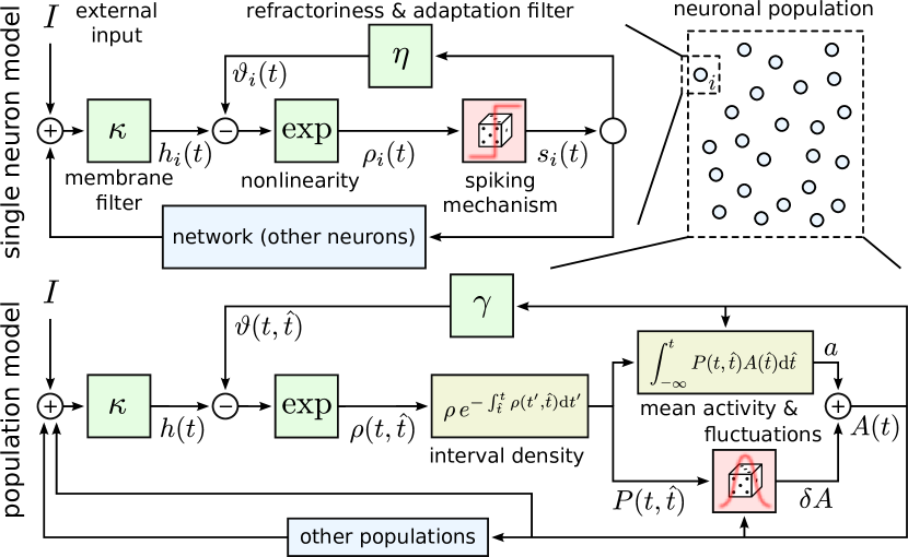
Figure 1: (Color) Schematic of the spike response model (a GLM for spike generation) with exponential escape noise and the derived quasi-renewal population model.

II Results

II.1 Dynamics of globally coupled renewal models. 

Our main quantity of interest is the population activity $A(t)=N^{-1}\sum_{i=1}^{N}s_{i}(t),$ where $s_{i}(t)=\sum_{k}\delta(t-t_{i}^{k})$ is the spike train of neuron $i$ with spike times $t_{i}^{k}$ and $N$ denotes the number of neurons. In experiments or simulations, the measured activity $\bar{A}(t)$ would be determined by temporal filtering of the population activity, i.e. $\bar{A}(t)=\int_{-\infty}^{\infty}A(t-s)f(s)\mathrm{d}s$ with a normalized filter function $f(s)$ with finite support. Below we will use a rectangular filter $f(s)=\theta(s)\theta(\Delta t-s)/\Delta t$, where $\theta(s)$ is the Heaviside step function.

To determine the fluctuation statistics of $A(t)$, we generalize the integral equation of an infinite population (Gerstner, 2000) to large but finite $N$. Let us first consider a homogeneous population of all-to-all connected renewal neurons. In this case, the spikes of each neuron occur with an instantaneous rate or hazard function $\rho_{\mathcal{H}}(t,\hat{t})$, which only depends on its last spike time $\hat{t}\leq t$ and the synaptic input determined by the history $\mathcal{H}(t)=\{A(t^{\prime})\}_{t^{\prime}<t}$ of the population activity. Note that for uncoupled stationary networks, the hazard reduces to $\rho_{\mathcal{H}}(t,\hat{t})=\rho(t-\hat{t})$ as it should be for a renewal model. The probability density of the next spike time $t$ given $\hat{t}$ is given by $P_{\mathcal{H}}(t,\hat{t})=\rho_{\mathcal{H}}(t,\hat{t})S_{\mathcal{H}}(t,\hat{t})$, with the survivor function defined as $S_{\mathcal{H}}(t,\hat{t})=\exp(-\int_{\hat{t}}^{t}\rho_{\mathcal{H}}(t^{\prime},\hat{t})dt^{\prime})$.

Our approach is to use the Gaussian approximation for large $N$, i.e. we calculate the first- and second-order statistics of $A(t)$ as a functional of its past activity (see Appendix B). However, the dynamics of $A$ depends on its own history $\mathcal{H}(t)$ and on the occupation density of refractory states $t-\hat{t}$ across the population (Meyer and van Vreeswijk, 2002). Thus, we have to average over the possible refractory states consistent with a given history $\mathcal{H}$. To perform the Gaussian approximation, the dynamics of the full system is coarse-grained by discretizing time with a small time step $\Delta t$ which is still large enough to include many spikes of the population. For large $N$, the number of neurons that fire in the time bin at $t$ and had their last spike in bin $\hat{t}$ is a Gaussian random number with mean and variance $n_{0}(\hat{t})P_{\mathcal{H}}(t,\hat{t})\Delta t$, where $n_{0}(\hat{t})=N\int_{\hat{t}}^{\hat{t}+\Delta t}A(s)\,ds$ is the past spike count at $\hat{t}<t$. Summing over $\hat{t}$ and treating $\Delta t$ as macroscopically infinitesimal, we find the conditional mean activity (see Appendix B)

$$a(t) =\int_{-\infty}^{t}P_{\mathcal{H}}(t,\hat{t})A(\hat{t})\,\mathrm{d}\hat{t},$$ (1)

which is equal to the population integral (Gerstner, 2000) for the infinite system. For finite $N$, $A(t)$ will be of the form

$$A(t) =a(t)+\delta A(t),$$ (2)

where the deviation $\delta A(t)$ has zero mean and a diverging standard deviation $\sqrt{a(t)/(N\Delta t)}$ because the variance of the spike count in $[t,t+\Delta t]$ is given by $N\Delta t\,a(t)$. Importantly, $\delta A(t)$ cannot be described by a white noise process but future values $\delta A(t+\tau)$, $\tau>0$, are correlated with $\delta A(t)$, because they share a common history $\mathcal{H}(t)$. In fact, a neuron that fired its last spike at $\hat{t}<t$ cannot have its next spike at both times $t$ and $t+\tau$, which induces a negative correlation for the deviations at $t$ and $t+\tau$. We find (see Appendix B) for $\tau\geq 0$ the conditional correlation function

$$\langle\delta A(t+\tau)\delta A(t)\rangle_{\mathcal{H}(t)}=N^{-1}a(t)\delta(\tau)-\\ N^{-1}\int_{-\infty}^{t}P_{\mathcal{H}}(t+\tau,\hat{t})P_{\mathcal{H}}(t,\hat{t})A(\hat{t})\,\mathrm{d}\hat{t},$$ (3)

where $\langle\cdot\rangle_{\mathcal{H}(t)}$ denotes the average conditioned on the history of $A$ before $t$. Thus, the correlation function is in general explicitly time-dependent.

II.2 Adaptation and random connectivity. 

In the presence of adaptation, the instantaneous rate of a neuron depends on all its previous spikes so that it can no longer be described by renewal theory. Here we describe how adapting neurons in networks may still be approximated by a quasi-renewal process. Specifically, we consider a homogeneous population of neurons modeled by the spike-response model with escape-noise (Gerstner, 2000), also known as GLM (Pillow et al., 2008; Truccolo et al., 2010; Mensi et al., 2012), with hazard function

$$\rho_{i}(t) =c\exp\left[(h_{i}(t)-\vartheta_{i}(t))/\delta u\right],$$ (4)

(Fig. 1). That is, neuron $i$ produces a spike in a small time interval $[t,\Delta t)$ with probability $\rho_{i}(t)\Delta t$. This probability depends on the input potential $h_{i}(t)=\left[\kappa\ast\left(\sum_{j=1}^{N}w_{ij}s_{j}(t)+I\right)\right](t)$, which is driven by presynaptic spike trains $s_{j}(t)$ (with synaptic weight $w_{ij}$) and external input $I(t)$. The membrane filter kernel is given by $\kappa(t)=\theta(t-\tau_{\mathrm{s}})\exp(-(t-\tau_{\mathrm{s}})/\tau_{\mathrm{m}})$, where $\tau_{\mathrm{s}}$ and $\tau_{\mathrm{m}}$ are the synaptic delay and the membrane time constant, respectively. The operation $\ast$ denotes the convolution $(f\ast g)(t)=\int_{-\infty}^{\infty}f(t-s)g(s)\mathrm{d}s$ and $\theta(t)$ is the Heaviside step function. The variable $\vartheta_{i}$ defined as $\vartheta_{i}(t)=(s_{i}\ast\eta)(t)$ can be interpreted as a dynamic firing threshold that is triggered by the neuron’s own output spike train $s_{i}(t)$ (Mensi et al., 2012). Here, $\eta(t)$ is a feedback kernel that consists of two parts, $\eta=\eta_{\mathrm{a}}+\eta_{\mathrm{r}}$: a short-range refractory kernel $\eta_{\mathrm{r}}(t)=\theta(t)\left[J_{\mathrm{r}}\theta(t-\tau_{\mathrm{abs}})\exp(-(t-\tau_{\mathrm{abs}})/\tau_{\mathrm{m}})+\theta(\tau_{\mathrm{abs}}-t)D\right]$ mainly affected by the last spike, and a long-range adaptation kernel $\eta_{\mathrm{a}}(t)=J_{\mathrm{a}}\theta(t)\exp(-t/\tau_{\mathrm{a}})$ that accumulates the spike history on a longer time scale $\tau_{\mathrm{a}}$. An absolute refractory period is included in $\eta_{\mathrm{r}}(t)$ by setting it to $D=10^{12}$ for $0<t<\tau_{\mathrm{abs}}$. Our choice of the kernels corresponds to a leaky IF model with dynamic threshold (Liu and Wang, 2001) and a reset by a constant amount $-J_{\mathrm{r}}$ after each spike.

The parameter $c$ in Eq. (4) sets a baseline firing rate and $\delta u$ sets the strength of intrinsic noise (“softness” of threshold). Fits of this model to pyramidal neuron recordings yielded $\delta u\approx 4\mathrm{mV}$ (Jolivet et al., 2006). Our standard parameter set given below corresponds to an amplitude of single post-synaptic potentials of $0.25\mathrm{mV}$ (excitatory, exc.) and $-1.1\mathrm{mV}$ (inhibitory, inh.). In the following, we measure voltage in units of $\delta u$, so that $\delta u=1$ in dimensionless units. For the synaptic weights $w_{ij}$, we use a homogeneous random network as specified in Appendix A, below.

The dependence of the term $\exp(-\vartheta_{i})$ in Eq. (4) which describes the feedback of the neuron’s own spiking history $s_{i}$ can be approximated by the explicit contribution of the last spike of the neuron at $\hat{t}$ and the average effect of previous spikes up to $\hat{t}$ (Naud and Gerstner, 2012):

$$e^{-\vartheta_{i}(t)} \approx e^{-\eta(t-\hat{t})}\langle e^{-\int_{-\infty}^{\hat{t}}s_{i}(t^{\prime})\eta(t-t^{\prime})\,\mathrm{d}t^{\prime}}\rangle_{t_{i}^{k}<\hat{t}}.$$

Here, the average is taken over all previous spike times $t_{i}^{k}<\hat{t}$. As shown in (Naud and Gerstner, 2012), this average can be approximated by $\exp\left[\int_{-\infty}^{\hat{t}}\left(e^{-\eta(t-t^{\prime})}-1\right)\langle s_{i}(t^{\prime})\rangle\,dt^{\prime}\right]$. Replacing further the firing rate $\langle s_{i}(t^{\prime})\rangle$ by the population activity $A(t^{\prime})$, the threshold $\vartheta_{i}(t)$ becomes

$$\vartheta(t,\hat{t}) =\eta(t-\hat{t})+(\gamma_{t-\hat{t}}\ast A)(t),$$ (5)

for all neurons with last spike at $\hat{t}$. The kernel $\gamma_{\tau}(s)=\theta(s-\tau)(1-e^{-\eta(s)})$ represents the effect of adaptation in the quasi-renewal (QR) approximation. Furthermore, for homogeneous random networks and large $N$, the local field $h_{i}$ caused by synaptic input to neuron $i$ is determined by $A$ and an effective weight $\bar{w}=N^{-2}\sum_{i,j}w_{ij}$ (Brunel and Hakim, 1999), hence

$$h(t) =[\kappa\ast(J_{\mathrm{s}}A+I)](t),$$ (6)

where $J_{\mathrm{s}}=N\bar{w}$. The above steps enable us to treat neuronal adaptation and network coupling in a quasi-renewal framework with hazard function

$$\rho_{\mathcal{H}}(t,\hat{t}) =c\exp\left[h(t)-\vartheta(t,\hat{t})\right].$$ (7)

Note that $\rho_{\mathcal{H}}(t,\hat{t})$ is identical for all neurons which have fired their last spike at $\hat{t}$.

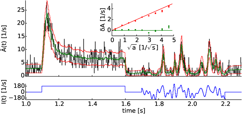
Figure 2: (Color) Quasi-renewal approximation of the population dynamics. Coarse-grained population activity $\bar{A}(t)$ ($\bar{A}(t)=n_{0}(t)/(N\Delta t)$, where $n_{0}(t)$ is the spike count in $[t,t+\Delta t)$, with $\Delta t=2\mathrm{ms}$, black) resulting from 500 randomly connected adapting neurons (4) receiving a common input current ($I(t)$, blue). The theoretical expectation $a(t)$ (green, Eq. 1) based on QR approximation (7), and expected fluctuations (red, one std., $a(t)\pm(N\Delta t)^{-\frac{1}{2}}a(t)^{\frac{1}{2}}$). At time $t$, $a(t)$ depends on the actual history $\bar{A}(t^{\prime})$ (black) for $t^{\prime}<t$. Standard parameters (see Appendix A), except for $I(t)$ as shown and $c=5\mathrm{s}^{-1}$. Inset shows mean (green) and std. (red) of deviations $\delta A(t)=\bar{A}(t)-a(t)$ as a function of $\sqrt{a}$, averaged over $25$ repetitions of the displayed $I(t)$ (dots) vs. theory (lines).

In Fig. 2 the population activity of a spiking neural network simulation is compared to the theoretical prediction (2). To evaluate (1) numerically, we iteratively compute $S_{\mathcal{H}}(t+\Delta t,\hat{t})=S_{\mathcal{H}}(t,\hat{t})(1-\rho_{\mathcal{H}}(t,\hat{t})\Delta t)$, with $S_{\mathcal{H}}(t,t)=1$, and use $P_{\mathcal{H}}=\rho_{\mathcal{H}}S_{\mathcal{H}}$. The QR population integral describes the response of the population activity and its fluctuations for stationary, as well as for slowly or rapidly varying inputs.

II.3 Linearized population dynamics. 

The amount of information transmitted and processed in sensory areas of the brain is limited by the fluctuations of the population activities (Zohary et al., 1994; Mar et al., 1999; Sompolinsky et al., 2001). Likewise, in decision networks, finite-size induced fluctuations determine the reliability of decisions (Wang, 2002; Deco and Rolls, 2006). The spontaneous activity of cortical networks is typically asynchronous, and is believed to underlie cortical information processing (Renart et al., 2010). In order to analytically determine the power spectrum of the spontaneous population activity, we linearize the dynamics around the large $N$ limit. To this end, we assume that in the limit $N\rightarrow\infty$ and for constant external input $I(t)=I_{0}$ the network dynamics has an equilibrium point with activity $A_{0}$ corresponding to an asynchronous firing state. With this equilibrium activity we can associate a renewal neuron model that is obtained from the original model, Eq. (4), by replacing $h_{i}(t)$ and $\vartheta_{i}(t,\hat{t})$ by $h_{0}=\kappa\ast(JA_{0}+I_{0})$ and $\vartheta_{0}(t-\hat{t})=\eta(t-\hat{t})+(\gamma_{t-\hat{t}}\ast A_{0})$, respectively. In the following, we will use the subscript “$0$” to refer to quantities of the associated renewal model. For finite system size, $N<\infty$, the activity will deviate from $A_{0}$. Through (5) and (6) the fluctuations $\Delta A(t)=A(t)-A_{0}$ also lead to fluctuations $\Delta h(t)=h(t)-h_{0}(t)$ and $\Delta\vartheta(t,\hat{t})=\vartheta(t,\hat{t})-\vartheta_{0}(t-\hat{t})$ , which in turn influence $A(t)$. Our goal is to determine the spectral properties of $\Delta A(t)$.

To simplify the derivations, we approximate the QR kernel $\gamma_{\tau}$ by its average over the inter-spike-interval density $P_{0}(\tau)$ ,

$$\gamma(s) = \int_{0}^{\infty}P_{0}(\tau)\gamma_{\tau}(s)\mathrm{d}\tau=(1-e^{-\eta(s)})(1-S_{0}(s))\,.$$ (8)

Expanding (1)-(3) to first order in $\Delta A$, $\Delta h$ and $\Delta\vartheta$, yields the linearized stochastic dynamics (see Appendix C)

$$A(t) = A_{0}+(Q\ast\Delta A)(t)+\sqrt{A_{0}/N}\xi(t).$$ (9a)

Here, $$Q(t)=P_{0}(t)+A_{0}\frac{\mathrm{d}}{\mathrm{d}t}(\mathcal{L}\ast[\kappa J_{\mathrm{s}}-\gamma])(t) a \Delta A \mathcal{L} \mathcal{L}(t)=\theta(t)\int_{0}^{\infty}\rho_{0}(s)S_{0}(s+t)\mathrm{d}s \mathcal{L} \xi(t)$$ determines the linear response of the expected activity to a perturbation . For our model (4), the kernel in this expression is given by but can be derived for most common neuron models (Gerstner, 2000), or, alternatively, may be estimated from neural recordings. The noise term is stationary Gaussian noise with correlation function

$$\langle\xi(t)\xi(t+\tau)\rangle =\delta(\tau)-\int_{0}^{\infty}P_{0}(s+\tau)P_{0}(s)\mathrm{d}s$$ (9b)

for all $\tau$; cf. (3). Eq. (9) shows that the population activity in the stationary state is a Gaussian process with memory, where finite-size fluctuations are described by the colored noise $\xi(t)$.

II.4 Fluctuations in coupled populations. 

Let us now turn to $K$ populations consisting of $\vec{N}=(N_{1},\dots,N_{K})$ neurons. Parameters of neurons and coupling are homogeneous within each population but may differ between one group and the next. To incorporate network coupling, the network input (6) becomes $h{}_{k}(t)=(\kappa_{k}\ast(\mathbf{J}\vec{A})_{k})(t)$ for $k=1,\dotsc,K$, where $\mathbf{J}$ is the coupling matrix and $\vec{A}(t)$ is a vector of population activities. For each population the dynamics are given by (9) but $\mathbf{Q}(t)$ is now a $K\times K$ matrix of coupling kernels. Using the Fourier transform $\tilde{f}(\omega)=\int_{-\infty}^{\infty}f(t)e^{-i\omega t}\mathrm{d}t$, this matrix can be written as $\tilde{\mathbf{Q}}(\omega)=\tilde{\mathbf{P}}_{0}+i\omega\mathbf{A}_{0}\tilde{\mathbf{L}}(\tilde{\mathbf{K}}\mathbf{J}-\tilde{\mathbf{G}})$, where the matrices $\mathbf{P}_{0},\mathbf{A}_{0},\mathbf{L},\mathbf{K},\mathbf{G}$ are defined as the diagonal matrices of the vectors $\vec{P}_{0},\vec{A}_{0},\vec{\mathcal{L}},\vec{\kappa},\vec{\gamma}$, respectively. The power spectrum, defined as the Fourier transform of the correlation function $\mathbf{C}_{A}(\tau)=\langle\Delta\vec{A}(t)\Delta\vec{A}^{T}(t+\tau)\rangle$, can be obtained from the transformed Eq. (9) as $\tilde{\mathbf{C}}_{A}(\omega)=(\mathbf{1}-\tilde{\mathbf{Q}})^{-1}\mathbf{N}^{-1}\mathbf{A}_{0}(\mathbf{1}-\tilde{\mathbf{P}}_{0}\tilde{\mathbf{P}}_{0}^{\dagger})(\mathbf{1}-\tilde{\mathbf{Q}}^{\dagger})^{-1}$. Here, ^† denotes the adjoint matrix (conjugate transpose). It is instructive to rewrite this expression in terms of the power spectrum of the associated renewal model (Stratonovich, 1963) $\tilde{\mathbf{C}}_{0}(\omega)=\mathbf{A}_{0}(\mathbf{1}-\tilde{\mathbf{P}}_{0})^{-1}(\mathbf{1}-\tilde{\mathbf{P}}_{0}\tilde{\mathbf{P}}_{0}^{\dagger})(\mathbf{1}-\tilde{\mathbf{P}}_{0}^{\dagger})^{-1}$ as follows:

$$\tilde{\mathbf{C}}_{A}(\omega) =\tilde{\mathbf{B}}\mathbf{N}^{-1}\tilde{\mathbf{C}}_{0}\tilde{\mathbf{B}}^{\dagger},\,\,\,\,\,\,\tilde{\mathbf{B}}=\left[\mathbf{1}-\tilde{\mathbf{R}}_{0}(\mathbf{J}-\tilde{\mathbf{K}}^{-1}\tilde{\mathbf{G}})\right]^{-1}$$ (10)

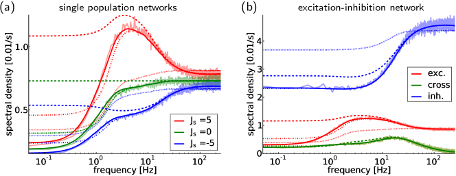
Figure 5: (Color) Spectral density of the population activity in random networks (as Fig. 3(a)-(b)) with comparison to earlier theories (special cases). Simulation (light colored lines) vs. theory (10) (solid lines). For comparison: uncoupled renewal processes ($\tilde{\mathbf{B}}=\mathbf{1}$), dotted; coupled renewal processes ($\tilde{\mathbf{B}}^{-1}=\mathbf{1}-\tilde{\mathbf{R}}_{0}\mathbf{J}$), dash-dotted; Hawkes process ($\tilde{\mathbf{B}}^{-1}=\mathbf{1}-\tilde{\mathbf{R}}_{0}\mathbf{J}$, $\tilde{\mathbf{C}}_{0}=\mathbf{A}_{0}$), dashed lines. (a): single populations ($K=1$), (b): coupled exc.-inh. network ($K=2$). Blue dash-dotted and solid lines coincide because inhibitory neurons here have no adaptation ($J_{\mathrm{a}}=0$). Standard parameters were used except as indicated.

Here, $\tilde{\mathbf{R}}_{0}=i\omega(\mathbf{1}-\tilde{\mathbf{P}}_{0})^{-1}\tilde{\mathbf{A}}_{0}\tilde{\mathbf{L}}\tilde{\mathbf{K}}$ is the diagonal matrix containing the linear response functions of the associated renewal models with respect to current perturbations $\vec{I}(t)$ (Gerstner, 2000). Eq. (10) shows that finite-size fluctuations are characterized by the renewal spectrum $\tilde{\mathbf{C}}_{0}(\omega)$, shaped by recurrent input (via $\mathbf{J}$ and $\tilde{\mathbf{K}}$) and adaptation (via $\tilde{\mathbf{G}}$), and reduced by the factor $\mathbf{N}^{-1}$. There are several known limit cases: first, for vanishing adaptation, $\tilde{\mathbf{G}}=0$, we recover the linear response result of (Lindner et al., 2005; Ávila Åkerberg and Chacron, 2009; Trousdale et al., 2012) for networks of white-noise driven IF neurons. Our formula shows that adaptation appears as an additional diagonal term in the effective coupling matrix $\mathbf{J}-\tilde{\mathbf{K}}^{-1}\tilde{\mathbf{G}}$, and hence can be interpreted as an inhibitory self-coupling. Second, if both adaptation and recurrent connections vanish, $\tilde{\mathbf{G}}=0$ and $\mathbf{J}=0$, we arrive at $\tilde{\mathbf{C}}_{A}(\omega)=\mathbf{N}^{-1}\tilde{\mathbf{C}}_{0}(\omega)$ because the superposition of independent spike trains does not change the shape of the power spectrum. Third, our result also includes the frequently employed Hawkes process (Hawkes, 1971; Pernice et al., 2012; Helias et al., 2013), which is recovered for a constant single neuron spectrum $\tilde{\mathbf{C}}_{0}=\mathbf{A}_{0}$ and vanishing adaptation, $\tilde{\mathbf{G}}=0$. For a comparison of our result to simulations, see Fig. 3, which will be discussed below. In section II.6 we make use of Eq. (10) to quantify information filtering in neural populations (Fig. 4). A comparison to the special cases of Eq. (10) described above is shown in Fig. 5.

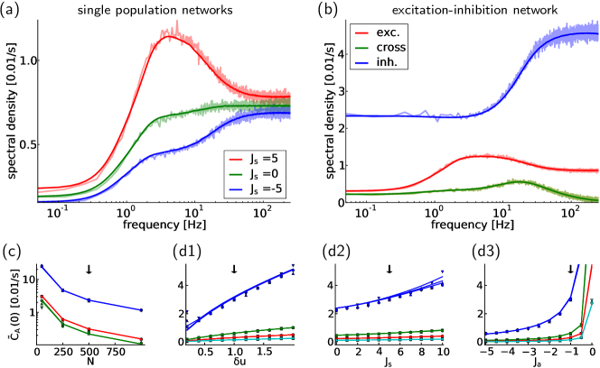
Figure 3: (Color) Spectral density of the population activity in random networks. Simulation (light colored lines) vs. theory (10) (solid lines). (a): single populations ($K=1$), (b-d): coupled exc.-inh. network ($K=2$), (in (b) green lines show the amplitude of the cross-spectrum). (c-d): The limit $\omega\to 0$ in dependence on parameters for the $K=2$ case shown in (b); symbols mark simulation results for different connection probabilities ($\bigtriangledown,\bigtriangleup,\circ$: $p=0.2,\,0.5,\,1$) while keeping $J_{\mathrm{s}}=N\bar{w}$ fixed, solid lines show theory (10). Symbols mostly fall on top of each other indicating independence of results with respect to $p$. In (c) colors are as in (b), in (d1-d3) only exc. population is shown, colors denote number of neurons (blue, green, red, cyan: $N=50,\,250,\,500,\,1000)$. Standard parameters (marked by arrows in (c-d), cf. Appendix A) were used except as indicated.

In Fig. 3(a)-(b) the spectral density is shown compared to simulations, where the frequency equals $\omega/(2\pi)$. The spectra are well described by the novel theory, which captures refractoriness, recurrent feedback and the reduction of power at low frequencies due to adaptation. The latter arises from negative correlations between ISIs typical for adapting neurons (Schwalger and Lindner, 2013). Interestingly, this purely non-renewal effect is well accounted for by our quasi-renewal theory. Since adaptation effects are most prominent at low frequency, we examined the dependence of the power on the model parameters for $\omega\to 0$ (Fig. 3(c)-(d)). Our theory describes the simulations well across the studied parameter range.

II.5 Influence of correlated external signals. 

Neuronal networks in the brain are subject to external influences, either due to sensory input or ongoing activity in other brain areas. How do neuronal populations respond to small, time-dependent input currents $\vec{I}(t)=(I_{1},\dots,I_{L})$ with spectral density $\tilde{\mathbf{C}}_{I}(\omega)$? To answer this question, we proceed as before and linearize Eqs. (1)-(3) with respect to the small fluctuations $\Delta h_{k}(t)=(\kappa_{k}\ast(\mathbf{J}\Delta\vec{A}+\mathbf{M}\vec{I})_{k})(t)$ of the local field. Here, we restrict our analysis to independent inputs $\vec{I}$, such that $\tilde{\mathbf{C}}_{I}$ is diagonal with entries $\tilde{C}_{I,i}$, but also included a $K\times L$ mixing matrix $\mathbf{M}$, which allows us to model shared input. The resulting spectral density is given by the sum

$$\tilde{\mathbf{C}}_{A}(\omega)= \tilde{\mathbf{B}}[\mathbf{N}^{-1}\tilde{\mathbf{C}}_{0}+\tilde{\mathbf{R}}_{0}\mathbf{M}\tilde{\mathbf{C}}_{I}\mathbf{M}^{\dagger}\tilde{\mathbf{R}}_{0}^{\dagger}]\tilde{\mathbf{B}}^{\dagger}.$$ (11)

Thus, additional fluctuations due to the stimulus $\vec{I}$ are shaped by both the single neuron filter $\mathbf{\tilde{R}}_{0}\mathbf{M}$ and the network and adaptation filter $\mathbf{\tilde{B}}$ (10), combining the effects of recurrent connectivity and adaptation.

II.6 Information transmission. 

Our theory allows us to quantify the transmission of information from external input signals $\vec{I}(t)$ through a system of coupled neural populations. The coherence between the signal $j$ and the activity of population $i$

$$\Gamma_{ij}(\omega)=\frac{|\langle\tilde{I}_{j}^{\ast}(\omega)\tilde{A}_{i}(\omega)\rangle|^{2}}{\tilde{C}_{I,j}(\omega)(\tilde{\mathbf{C}}_{A}(\omega))_{ii}}$$ (12)

can be regarded as a frequency resolved measure of information transmission. Information theory (Shannon, 1948; Gabbiani, 1996; Borst and Theunissen, 1999) states that the mutual information rate is bounded from below by $-\int_{0}^{\infty}\log_{2}[1-\Gamma_{ij}(\omega)]\frac{\mathrm{d}\omega}{2\pi}$.

Since adaptation attenuates the response to slowly changing signals, one might expect that it also attenuates low frequency information content. For a single population, however, this is not the case, but instead the coherence is low-pass, i.e. it monotonically decreases for increasing frequency (Ávila Åkerberg and Chacron, 2009). Here we show that in coupled populations of adapting neurons, coherences can be non-monotonic allowing the neural circuit to preferentially encode information in certain frequency bands. Put differently, a multi-population setup can realize an information filter.

Using Eq. (12), we find the general form of the coherence matrix:

$$\Gamma_{ij}(\omega) =\frac{|(\tilde{\mathbf{B}}\tilde{\mathbf{R}}_{0}\mathbf{M})_{ij}|^{2}\tilde{C}_{I,j}}{\sum_{k=1}^{K}|\tilde{B}_{ik}|^{2}\tilde{C}_{0,k}+\sum_{l=1}^{L}|(\tilde{\mathbf{B}}\tilde{\mathbf{R}}_{0}\mathbf{M})_{il}|^{2}\tilde{C}_{I,l}}\,.$$ (13)

In this expression, the numerator represents the contribution of the signal $I_{j}(t)$ to the power spectrum of population $i$. This effective signal power is divided by the total power spectrum of population $i$, which consists of direct ($k=i$) and indirect ($k\neq i$) sources of variability. Both sources contain internally generated noise due to finite size $N_{k}$ as well as signal power. However, the diagonal elements ($k=i$) of the shaping matrices can be much stronger than the off-diagonal elements ($k\neq i$) depending on the coupling matrix $\mathbf{J}$. Therefore, we expect that the direct source of variability dominates in the denominator.

If there is only one population and signal ($K=1$, $L=1$), the term $|\tilde{B}_{11}(\omega)|^{2}$ occurs in both numerator and denominator and cancels. Thus, coupling and adaptation do not shape the coherence in a single population. Furthermore, the signal term $|\tilde{R}_{0,1}(\omega)|^{2}M_{11}\tilde{C}_{I,1}(\omega)$ is matched in both numerator and denominator, which leads to a flat coherence at frequencies where the signal dominates the finite $N$ noise. At high frequencies, the neural response amplitude $|\tilde{\mathbf{R}}_{0}|^{2}$ decays due to the leaky membrane, but the spontaneous spectrum $\tilde{\mathbf{C}}_{0}$ has a constant high-frequency limit equal to $\mathbf{A}_{0}$. One therefore typically observes a low-pass like information transfer characteristics of single neurons or populations (Chacron et al., 2004; Vilela and Lindner, 2009; Ávila Åkerberg and Chacron, 2009).

For several populations ($K>1$), however, we can distinguish two cases: If the signal is read out at a receiving population, $M_{ij}\neq 0$, the signal power in the numerator is matched by the dominating direct signal power in the denominator, and hence the shaping of the signal power cancels. In contrast, if read out at a different population, $M_{ij}=0$, the signal $j$ contributes only indirectly to the power spectrum of population $i$ via synaptic connections. Thus, we expect that the shape of signal power and power spectrum (i.e. numerator and denominator, respectively) is generally different if the transmission path involves multiple populations.

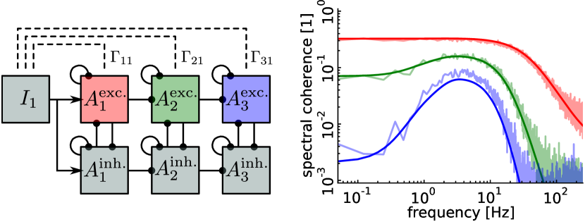
Figure 4: (Color) Signal processing and coherence shaping in a feed-forward chain of recurrently connected neural populations, simulation vs. theory. Left: Schematic of the network. Right: spectral coherences $\Gamma_{i1}$ (13) of $I_{1}$ and $A_{i}^{\mathrm{exc.}}$, theory (13) (lines) vs. simulation result (light colored lines). Colors indicate coherences of signals $I_{1}$ and population activity $A_{i}$. The mutual information rate is closely related to the spectral coherence, see text. Standard parameters, except for increased coupling $J_{\mathrm{s}}=10$. The input current $I_{1}(t)$ is a Gaussian white noise with spectral density $\tilde{C}_{I,1}(\omega)=9\mathrm{s}^{-1}$.

As an example of this mechanism, we show a feed-forward chain of excitatory and inhibitory populations (Fig. 4, $K=6$, $L=1$). In the first layer, the effective signal power is reduced at low frequencies because of adaptation and inhibitory feedback. However, the power spectrum of $A_{\mathrm{exc},1}(t)$ is dominated by the same signal power and hence exhibits a very similar reduction of low-frequency power. Consequently, the coherence (being the ratio of these two spectra) is rather flat at low frequencies and shows a decay at higher frequencies (Fig. 4, red lines). This low-pass characteristics changes at later stages in the chain (green & blue): The signal term is increasingly more shaped by adaptation and coupling properties, whereas the noise spectrum changes less. As a result, the coherence shows a maximum at a finite frequency (Fig. 4, blue lines). This band-pass structure becomes more pronounced from layer to layer, representing a form of information filtering. Coherence functions with band-pass characteristics have been observed in neurons postsynaptic to electro-receptor afferents in electric fish (Chacron et al., 2005; Krahe et al., 2008).

III Conclusions

We have shown that fluctuations in finite-sized networks of spiking neurons are captured by a colored noise term added to the population integral equation of the infinite system. Our approach yields spectral densities of the population activity in randomly or fully connected multi-population networks which are in excellent agreement with simulation results. Our quasi-renewal theory includes refractory effects and adaptation on multiple time scales. In contrast to earlier treatments of neuronal refractory effects in population dynamics (Toyoizumi et al., 2009; Pernice et al., 2012; Helias et al., 2013) or linear response formulas for adaptive neurons (Richardson, 2009), the QR population integral, derived directly from the neuron model definition, captures the time-dependent, non-linear dynamics and adaptation of neural population activity.

We applied our theory to information filtering by coupled populations of spiking neurons with adaptation. We showed that, although impossible in single populations due to a cancellation of signal and noise terms of the coherence, coupled populations can filter information through adaptation mechanisms and neuronal interactions. This mechanism might be exploited in the layered structure of cortical circuits, or in sensory systems of insects where signals traverse a sequence of nuclei.

In this paper we treated populations of point neurons with static synapses and applied linear response theory. How to generalize our theory to incorporate effects of nonlinear dendritic integration, spike-synchrony detection and short-term synaptic plasticity, which all contribute to information filtering (Rosenbaum et al., 2012; Sharafi et al., 2013; Droste et al., 2013), is an important question that merits further investigation. Nonetheless, due to the versatility of GLM models, our theory already provides a useful tool for interpreting neural data at the population level. For example, our theory suggests that in in-vitro experiments with optogenetically evoked input currents and simultaneous measurements of neural activity (El Hady et al., 2013), system parameters may be identified based on the relation of the spectra, Eq. (11). Moreover, large-scale neural systems can now be analyzed as coupled populations of model neurons with single-cell parameters extracted from experiments, and simulated using a muti-scale approach.

Appendix A Network simulations

We compare our theoretical results to simulations of networks of excitatory and inhibitory neurons defined by (4). In the case $K=1$ (Fig. 3(a)), we use $\vec{N}=N$ and $\mathbf{J}=J_{\mathrm{s}}$, in the case $K=2$ (Fig. 3(b)-(d)), $\vec{N}=(\nicefrac{{4}}{{5}}N,\nicefrac{{1}}{{5}}N)$, and $\mathbf{J}=((J_{\mathrm{s}},-1.1\,J_{\mathrm{s}}),(J_{\mathrm{s}},-1.1\,J_{\mathrm{s}}))$. In the case $K=6$ (Fig. 4), each exc. (inh.) population consists of $\nicefrac{{4}}{{5}}N$ ($\nicefrac{{1}}{{5}}N$) neurons and $\mathbf{J}$ with entries as in Fig. 4A, where exc. (inh.) couplings are $J_{\mathrm{s}}$ ($-1.1\,J_{\mathrm{s}}$). Generally, neurons of population $i$ receive synapses from a random subset of $pN_{j}$ neurons of population $j$, each with synaptic weight $w_{ij}=J_{ij}/(pN_{j})$ and delay $\tau_{\mathrm{s}}$. Unless the connection probability $p$ is $1$, self-connections are excluded. Networks were simulated for $2\cdot 10^{4}\mathrm{s}$ using NEST (Gewaltig and Diesmann, 2007) (neuron model pp_psc_delta, temporal resolution $2\mathrm{ms}$). Standard parameters, unless indicated otherwise: $N=500$, $c=10\mathrm{s}^{-1}$, $\tau_{\mathrm{m}}=0.01\mathrm{s}$, $\tau_{\mathrm{a}}=0.3\mathrm{s}$, $\Delta t=\tau_{\mathrm{s}}=\tau_{\mathrm{abs}}=2\mathrm{ms}$, $J_{\mathrm{r}}=3$, $J_{\mathrm{a}}=1$, $J_{\mathrm{s}}=5$, $p=0.2$, $I_{0}=0,$ $\tilde{C}_{I}=0$. In the exc.-inh. network, for the inh. neurons which typically show little adaptation (Mensi et al., 2012) we deactivated adaptation by setting $J_{\mathrm{a}}=0$ and $c=5\mathrm{s}^{-1}$. While it is possible to theoretically approximate the stationary interval distribution $P_{0}$ by searching for a self-consistent rate $A_{0}$ as described in (Naud and Gerstner, 2012), here we use $P_{0}$ from simulated inter-spike-intervals of each population. From the measured $P_{0}(t)$ we derive $A_{0}=1/\int_{0}^{\infty}tP_{0}(t)\mathrm{d}t$, $S_{0}(t)=\int_{t}^{\infty}P_{0}(t^{\prime})\mathrm{d}t^{\prime}$ and $\rho_{0}(t)=P_{0}(t)/S_{0}(t)$.

Appendix B Detailed derivation of Eq. (3)

The aim is to find a dynamical equation for the population activity

$$A(t)=\frac{1}{N}\sum_{i=1}^{N}s_{i}(t)=\lim_{\Delta t\rightarrow 0}\frac{n_{0}(t)}{N\Delta t},$$ (14)

where $n_{0}(t)$ is the total number of spikes in the interval $[t,t+\Delta t]$. More generally, we define $n_{k}(t)$, $k\in\mathbb{Z}$, as the total number of spikes in $[t-k\Delta t,t-(k-1)\Delta t]$, i.e. the activity $k$ time bins in the past. It is useful to consider furthermore the total number of neurons that spiked in the time bin $[t-k\Delta t,t-(k-1)\Delta t]$, $k=1,2,\dotsc$, but had no further spike until time $t$. Let us denote this number by $m_{k}(t)$ (Fig. 6 and Table 1). The number of neurons that spike in $[t,t+\Delta t]$ and had their last spike in the bin $[t-k\Delta t,t-(k-1)\Delta t]$ shall be denoted by $\delta m_{k}(t)$. These neurons decrease the number $m_{k}(t)$ of neurons from group $k$ that had survived until time $t+\Delta t$ in the next time step, i.e.

$$\delta m_{k}(t)=m_{k}(t)-m_{k+1}(t+\Delta t),\qquad k=1,2,\dotsc.$$ (15)

The total number of spikes at time $t$, $n_{0}(t)$, is the sum over all possible last spike times, hence

$$n_{0}(t)=\sum_{k=1}^{\infty}\delta m_{k}(t).$$ (16)

Figure 6: Illustration of negative correlations between $\delta m_{k}(t)$ and $\delta m_{k+1}(t+\Delta t)$. (a): Expected number of spikes from group $k$ in bins $[t,t+\Delta t]$ and $[t+\Delta t,t+2\Delta t]$. (b): A large fluctuation of $\delta m_{k}(t)$ leads to reduction of the number of available spikes $m_{k+1}(t+\Delta t)$. As a consequence, $\delta m_{k+1}(t+1)$ tends to be small.

We will now express the activity $n_{0}(t)$ in terms of the past activity $\mathcal{H}_{t}=\{n_{k}(t)\}_{k=1,2,\dotsc}$, using the Gaussian approximation. This requires to compute the mean and correlation function of $n_{0}(t)$ given the past values $n_{k}(t)$, $k=1,2,\dotsc$. In the following, the averaging bracket $\left\langle\cdot\right\rangle$ has to be understood as the conditional average $\left\langle\cdot\right\rangle_{\mathcal{H}_{t}}=\left\langle\cdot\right\rangle_{\{n_{k}(t)\}_{k=1,2,\dotsc}}$, i.e. we will omit the conditioning subscript for simplicity. Although $n_{k}(t)$, the total number of spikes in bin $t-k\Delta t$, is fixed, the number $m_{k}(t)$ of neurons that had their last spike in bin $t-k\Delta t$ is variable. It is this variability that we will average over (This corresponds to a statistical ensemble of populations that all have an identical history of population activity $n_{k}(t)$, $k=1,2,\dotsc$.).

$n_{0}(t)$	# of neurons which spike in $[t,t+\Delta t]$
$n_{k}(t)$	# of neurons which spiked in
	$[t-k\Delta t,t-(k-1)\Delta t]$ ; $n_{k}(t)=n_{0}(t-k\Delta t)$
$m_{k}(t)$	# of neurons with last spike in
	$[t-k\Delta t,t-(k-1)\Delta t]$
$\delta m_{k}(t)$	# of neurons with last spike in
	$[t-k\Delta t,t-(k-1)\Delta t]$ and next spike in $[t,t+\Delta t]$
$\rho(t,\hat{t})$	hazard function: rate at $t$ given last spike at $\hat{t}$
$S(t,\hat{t})$	survivor function: probability of no spike in $[\hat{t},t]$
$P(t,\hat{t})$	inter-spike-interval density: probability density
	of next spike at $t$ given last spike at $\hat{t}$;   $P=\rho\cdot S$

Table 1: Definitions of symbols used in Appendix B.

Suppose we know the value $m_{k}(t)$ of the group of neurons with their last spike in $[t-k\Delta t,t-(k-1)\Delta t]$. Then the expected number of spikes from that group in the next interval is

$$\langle\delta m_{k}(t)\rangle_{m_{k}(t)} =\rho(t,t-k\Delta t)\cdot\Delta t\cdot m_{k}(t)\,,$$ (17)

where $\rho(t,\hat{t})$ is the hazard function of the neurons (instantaneous rate at time $t$ given last spike at $\hat{t}$), and $\langle x\rangle_{y}$ denotes the expectation of $x$ conditioned on $y$ (in addition to the overall condition of a fixed history $\mathcal{H}_{t}=\{n_{k}(t)\}_{k=1,2,\dotsc}$). But since we do not know the exact value of $m_{k}(t)$ we need to average

$$\langle\delta m_{k}(t)\rangle =\langle\langle\delta m_{k}(t)\rangle_{m_{k}(t)}\rangle$$

$$=\rho(t,t-k\Delta t)\cdot\Delta t\cdot\langle m_{k}(t)\rangle$$ (18)

where we have used (17). We now use this result to calculate the expected number of spikes in the interval $[t,t+\Delta t]$. Averaging over (16) yields

$$\langle n_{0}(t)\rangle =\sum_{k=1}^{\infty}\rho(t,t-k\Delta t)\cdot\Delta t\cdot\langle m_{k}(t)\rangle\,.$$ (19)

The average number of neurons that fired their last spike in $[t-k\Delta t,t-(k-1)\Delta t]$ and survived up to $t$ can be expressed using the survival probability $S(t,\hat{t})=\exp(-\int_{\hat{t}}^{t}\rho(t^{\prime},\hat{t})dt^{\prime})$ as follows:

$$\langle m_{k}(t)\rangle =S(t,t-k\Delta t)n_{k}(t)$$

$$=S(t,t-k\Delta t)n_{0}(t-k\Delta t)\,.$$ (20)

We can now take the limit $\Delta t\to 0$ in (19) and find

$$\frac{\langle n_{0}(t)\rangle}{\Delta t} \to N\int_{-\infty}^{t}P(t,\hat{t})A(\hat{t})\,\mathrm{d}t^{\prime},\quad\Delta t\to 0,$$ (21)

where $P(t,\hat{t})=\rho(t,\hat{t})S(t,\hat{t})$ is the inter-spike-interval density. Eq. (21) is equivalent to Eq. (1).

To obtain the correlation function we can write for $q\in\mathbb{Z}$

$$\langle n_{0}(t)n_{0}(t+q\Delta t)\rangle=\sum_{k,l=1}^{\infty}\langle\delta m_{k}(t)\delta m_{l}(t+q\Delta t)\rangle.$$ (22)

Here, the spike numbers $\delta m_{k}(t)$ and $\delta m_{l}(t+q\Delta t)$ that refer to different groups $k$ and $l-q$ are uncorrelated. Correlations only arise for $\delta m_{k}(t)$ and $\delta m_{k+q}(t+q\Delta t)$, i.e. spikes that refer to the same group in the past. Thus,

$$\langle n_{0}(t)n_{0}(t+q\Delta t)\rangle=\sum_{k,l=1}^{\infty}\langle\delta m_{k}(t)\rangle\langle\delta m_{l}(t+q\Delta t)\rangle\\ +\sum_{k=1}^{\infty}\langle\delta m_{k}(t)\delta m_{k+q}(t+q\Delta t)\rangle\\ -\sum_{k=1}^{\infty}\langle\delta m_{k}(t)\rangle\langle\delta m_{k+q}(t+q\Delta t)\rangle,$$ (23)

so that the covariance is

$$\langle\Delta n_{0}(t)\Delta n_{0}(t+q\Delta t)\rangle=\sum_{k=1}^{\infty}\langle\delta m_{k}(t)\delta m_{k+q}(t+q\Delta t)\rangle\\ -\sum_{k=1}^{\infty}\langle\delta m_{k}(t)\rangle\langle\delta m_{k+q}(t+q\Delta t)\rangle,$$ (24)

where $\Delta n_{0}(t)=n_{0}(t)-\langle n_{0}(t)\rangle$. Therefore we need to compute

$$\langle\delta m_{k}(t)\delta m_{k+q}(t+q\Delta t)\rangle\,.$$ (25)

To this end, let us consider the cases $q=0$ and $q>0$ separately.

For $q=0$ and large $N$, the number of neurons that spike in $[t,t+\Delta t]$ and had their last spike at $t-k\Delta t$ is a Poisson variable with mean and variance $\Delta t\,P(t,\,t-k\Delta t)\,n_{k}(t)$. Thus (25) becomes

$$\left\langle[\delta m_{k}(t)]^{2}\right\rangle=\Delta t\,P(t,\,t-k\Delta t)\,n_{k}(t)+\mathcal{O}(\Delta t^{3}).$$ (26)

For $q>0$, we employ (15) twice and obtain

$$\langle\delta m_{k}(t)\delta m_{k+q}(t+q\Delta t)\rangle=\langle m_{k}(t)\,m_{k+q}(t+q\Delta t)\rangle\\ -\langle m_{k+1}(t+\Delta t)\,m_{k+q}(t+q\Delta t)\rangle\\ -\langle m_{k}(t)\,m_{k+q+1}(t+(q+1)\Delta t)\rangle\\ +\langle m_{k+1}(t+\Delta t)\,m_{k+q+1}(t+(q+1)\Delta t)\rangle.$$ (27)

In order to evaluate each of these four correlators, we note that the probability that a neuron from group $k$ “survives” until time $t+q\Delta t$ given that it survived until time $t$ is $S(t+q\Delta t,t-k\Delta t)/S(t,t-k\Delta t)$ according to Bayes law. Thus, out of the $m_{k}(t)$ neurons that survived until time $t,$ on average

$$\left\langle m_{k+q}(t+q\Delta t)\right\rangle{}_{m_{k}(t)}=\frac{S(t+q\Delta t,t-k\Delta t)}{S(t,t-k\Delta t)}\cdot m_{k}(t),$$ (28)

also survive until $t+q\Delta t$. Therefore, the correlator for $0\leq l<q$ can be written as

$$\left\langle m_{k+l}(t+l\Delta q)m_{k+q}(t+q\Delta t)\right\rangle=\\ =\left\langle m_{k+l}(t+l\Delta q)\left\langle m_{k+q}(t+q\Delta t)\right\rangle_{m_{k+l}(t+l\Delta t)}\right\rangle,\\ =\frac{S(t+q\Delta t,t-k\Delta t)}{S(t+l\Delta t,t-k\Delta t)}\cdot\left\langle m_{k+l}^{2}(t+l\Delta t)\right\rangle.$$

Applying this result to (27), we obtain

$$\langle\delta m_{k}(t)\delta m_{k+q}(t+q\Delta t)\rangle=\\ \left[S(t+(q+1)\Delta t,t-k\Delta t)-S(t+q\Delta t,t-k\Delta t)\right]\\ \times\left(\frac{\langle[m_{k+1}(t+\Delta t)]^{2}\rangle}{S(t+\Delta t,t-k\Delta t)}-\frac{\langle[m_{k}(t)]^{2}\rangle}{S(t,t-k\Delta t)}\right)$$ (29)

How can we calculate the second moment of $m_{k}(t)$? Recall that $m_{k}(t)$ is the part of the $n_{k}(t)$ neurons firing in bin $t-k\Delta t$ that survived until time $t$. Thus $m_{k}(t)$ can be regarded as a binomially distributed random number with $n=n_{k}(t)$ trials and survival probability $p=S(t,\,t-k\Delta t)$. This random number has mean $np$ and variance $np(1-p)$. Hence, the second moment reads

$$\langle[m_{k}(t)]^{2}\rangle=\langle[m_{k}(t)-\langle m_{k}(t)\rangle]^{2}\rangle+\underbrace{\langle m_{k}(t)\rangle^{2}}_{\mathcal{O}(\Delta t^{2})}\\ =n_{k}(t)S(t,\,t-k\Delta t)\left[1-S(t,\,t-k\Delta t)\right]+\mathcal{O}(\Delta t^{2}).$$ (30a)

Likewise,

$$\langle[m_{k+1}(t+\Delta t)]^{2}\rangle=n_{k}(t)S(t+\Delta t,t-k\Delta t)\\ \times\left[1-S(t+\Delta t,t-k\Delta t)\right]+\mathcal{O}(\Delta t^{2})$$ (30b)

because $n_{k+1}(t+\Delta t)=n_{k}(t)$. Inserting (30a) into (29) we find

$$\langle\delta m_{k}(t)\delta m_{k+q}(t+q\Delta t)\rangle=n_{k}(t)\,\Delta t^{2}\\ \times\frac{S(t+(q+1)\Delta t,t-k\Delta t)-S(t+q\Delta t,t-k\Delta t)}{\Delta t}\\ \times\frac{S(t,t-k\Delta t)-S(t+\Delta t,t-k\Delta t)}{\Delta t}\\ =-P(t+q\Delta t,t-k\Delta t)P(t,\,t-k\Delta t)\,n_{k}(t)\,\Delta t^{2}\,,.$$ (31)

Here, we have identified the derivative $\nicefrac{{\mathrm{d}}}{{\mathrm{d}t}}S(t,\hat{t})=-P(t,\hat{t})$. Note that this expression is of order $\mathcal{O}(\Delta t^{3})$, whereas $\langle\delta m_{k}(t)\rangle\langle\delta m_{k+q}(t+q\Delta t)\rangle$ is of order $\mathcal{O}(\Delta t^{4})$. So we can neglect the second term on the right-hand side of Eq. (24).

Putting all together, we find

$$\frac{1}{\Delta t^{2}}\langle\Delta n_{0}(t)\Delta n_{0}(t^{\prime}=t+q\Delta t)\rangle\\ =\frac{1}{\Delta t^{2}}\sum_{k=1}^{\infty}\langle\delta m_{k}(t)\delta m_{k+q}(t+q\Delta t)\rangle\\ =\frac{1}{\Delta t}\delta_{q,0}\left[\sum_{k=1}^{\infty}P(t,\,t-k\Delta t)n_{k}(t)+\mathcal{O}(\Delta t)\right]\\ -\sum_{k=1}^{\infty}P(t+q\Delta t,\,t-k\Delta t)P(t,\,t-k\Delta t)n_{k}(t)\\ \xrightarrow[\Delta t\to 0]{}\,N\delta(t-t^{\prime})\int_{-\infty}^{t}P(t,t^{\prime\prime})A(t^{\prime\prime})\,\mathrm{d}t^{\prime\prime}\\ -N\int_{-\infty}^{t}P(t,t^{\prime\prime})P(t^{\prime},t^{\prime\prime})A(t^{\prime\prime})\,\mathrm{d}t^{\prime\prime}.$$ (32)

Thus, using (21), we arrive at the final result

$$A(t)=\int_{-\infty}^{t}P(t,t^{\prime})A(t^{\prime})\,\mathrm{d}t^{\prime}+\delta A(t)$$ (33)

where $\delta A(t)$ is Gaussian with conditional correlation function

$$\langle\delta A(t)\delta A(t+\tau)\rangle=N^{-1}\delta(\tau)\int_{-\infty}^{\infty}P(t,t^{\prime})A(t^{\prime})\,\mathrm{d}t^{\prime}\\ -N^{-1}\int_{-\infty}^{\infty}P(t+\tau,t^{\prime})P(t,t^{\prime})A(t^{\prime})\,\mathrm{d}t^{\prime}$$ (34)

for $\tau\geq 0$. In the latter expression we extended the limits of integration to infinity, which is possible if we assume $P(t,t^{\prime})=0$ for $t<t^{\prime}$. Equation (34) tells us that the noise correlation function consists of two parts: a white ($\delta$-correlated) part and a negative correlation due to neural refractoriness. Intuitively, since $\delta m_{k}(t)$ and $\delta m_{k+1}(t+\Delta t)$ share the same number of available neurons $m_{k}(t)$, a positive fluctuation of the number of spikes in the bin $t$ of the neurons of group $k$ reduces the number of neurons with last spike in bin $k$ more than on average. Thus, the number of neurons of group $k$ that can still fire in time bin $t+\Delta t$ is smaller than on average, which explains the negative correlations (Fig. 6).

Appendix C Detailed derivation of Eq. (9)

We aim to linearize the population integral $a(t)=\int_{-\infty}^{t}P(t,\hat{t})A(\hat{t})\,\mathrm{d}\hat{t}$, Eq. (1), around an equilibrium point $A_{0}$, with small fluctuations $\Delta A(t)=A(t)-A_{0}$ with a mean of zero. To this end, let us first note that the hazard function Eq. (7) then can be written as

$$\rho(t,\hat{t}) =ce^{h_{0}-\vartheta_{0}(t-\hat{t})}e^{\Delta h(t)-\Delta\vartheta(t,\hat{t})}=\rho_{0}(t-\hat{t})e^{\Delta g(t,\hat{t})}.$$ (35)

Furthermore, recall that $P(t,\hat{t})=-\nicefrac{{\mathrm{d}}}{{\mathrm{d}t}}S(t,\hat{t})$, where $S(t,\hat{t})=\exp\left(-\int_{\hat{t}}^{t}\rho(s,\hat{t})\mathrm{d}s\right)$. Expanding to first order in $\Delta A$ yields $S(t,\hat{t})=S_{0}(t-\hat{t})+\Delta S(t,\hat{t})$ and $P(t,\hat{t})=P_{0}(t-\hat{t})-\nicefrac{{\mathrm{d}}}{{\mathrm{d}t}}\Delta S(t,\hat{t})$, where $S_{0}(t)=\exp(-\int_{0}^{t}\rho_{0}(t^{\prime})\mathrm{d}t^{\prime})$ and $P_{0}(t)=-\nicefrac{{d}}{{dt}}S_{0}(t)$ define the zeroth-order terms. Thus, the linearized population integral reads

$$a(t) =A_{0}+(P_{0}\ast\Delta A)(t)-A_{0}\frac{\mathrm{d}}{\mathrm{d}t}\int_{-\infty}^{t}\Delta S(t,\hat{t})\,\mathrm{d}\hat{t},$$ (36)

where we used the normalization of $P_{0}(t)$ and the boundary condition $\Delta S(t,t)=0$.

The perturbation is given by

$$\Delta S(t,\hat{t}) =\int_{-\infty}^{\infty}\left.\frac{\delta S(t,\hat{t})}{\delta\Delta g(s,\hat{t})}\right|_{\Delta g=0}\cdot\Delta g(s,\hat{t})\,\mathrm{d}s.$$

The functional derivative at $\Delta g=0$ reads

$$\left.\frac{\delta S(t,\hat{t})}{\delta\Delta g(s,\hat{t})}\right|_{\Delta g=0} =\left.\frac{\delta\exp\left(-\int_{\hat{t}}^{t}\rho_{0}(t^{\prime}-\hat{t})e^{\Delta g(t^{\prime},\hat{t})}dt^{\prime}\right)}{\delta\Delta g(s,\hat{t})}\right|_{\Delta g=0}$$

$$=-\theta(t-s)\theta(s-\hat{t})S_{0}(t,\hat{t})\rho_{0}(s-\hat{t}).$$

We insert this expression to compute the integral in (36)

$$-\int_{-\infty}^{t}\Delta S(t,\hat{t})\mathrm{d}\hat{t}=\int_{-\infty}^{t}\int_{-\infty}^{\infty}\theta(s-\hat{t})\theta(t-s)\\ \times S_{0}(t-\hat{t})\rho_{0}(\underbrace{s-\hat{t}}_{x(\hat{t})})\Delta g(s,\hat{t})\,\mathrm{d}s\,\mathrm{d}\hat{t}\\ =\int_{-\infty}^{\infty}\theta(t-s)\int_{0}^{\infty}\theta(x)S_{0}(t-s+x)\rho_{0}(x)\Delta g(s,s-x)\mathrm{d}x\mathrm{d}s\\ \overset{[8]}{=}\int_{-\infty}^{\infty}\Delta g(s)\underbrace{\theta(t-s)\int_{0}^{\infty}\theta(x)S_{0}(t-s+x)\rho_{0}(x)\,\mathrm{d}x}_{\mathcal{L}(t-s)}\,\mathrm{d}s\,.$$

In the last step, we have used the approximation Eq. (8), $\Delta g(t,\hat{t})=\Delta g(t)=[(\kappa J_{\mathrm{s}}-\gamma)\ast\Delta A](t)$, which has no dependence on the time of the last spike. Hence (36) becomes

$$a(t) =A_{0}+(P_{0}\ast\Delta A)(t)+A_{0}\frac{\mathrm{d}}{\mathrm{d}t}(\mathcal{L}\ast\Delta g)(t).$$ (37)

This linearized equation for the mean activity is valid for any small $\Delta A$ and $\Delta g$ in the past, also if due to finite size fluctuations. Eqs. (35)-(37) generalize to additional time-dependent inputs $\Delta I(t)$ by extending the definition of $\Delta g$ to $\Delta g(t)=[(\kappa J_{\mathrm{s}}-\gamma)\ast\Delta A+\kappa\ast\Delta I](t)$.

Furthermore, the noise correlation function Eq. (34) becomes to leading order

$$\langle\xi(t+\tau)\xi(t)\rangle=\delta(\tau)-\int_{-\infty}^{t}P_{0}(t+\tau-\hat{t})P_{0}(t-\hat{t})\,\mathrm{d}\hat{t},$$ (38)

with $\sqrt{A_{0}/N}\xi(t)=\delta A(t)$. Eqs. (37) and (38) are equivalent to Eq. (9).

References

- Klein and Shinoda (2008) M. L. Klein and W. Shinoda, Science 321, 798 (2008).
- Ayton et al. (2007) G. S. Ayton, W. G. Noid, and G. A. Voth, Curr Opin Struct Biol 17, 192 (2007).
- Peter and Kremer (2009) C. Peter and K. Kremer, Soft Matter 5, 4357 (2009).
- Pielke (2002) R. A. Pielke, Mesoscale Meteorological Modeling (Academic Press, 2002).
- Benaïm and Le Boudec (2008) M. Benaïm and J.-Y. Le Boudec, Perform Evaluation 65, 823 (2008).
- Gerstner et al. (2012) W. Gerstner, H. Sprekeler, and G. Deco, Science 338, 60 (2012).
- Lefort et al. (2009) S. Lefort, C. Tomm, J.-C. F. Sarria, and C. C. H. Petersen, Neuron 61, 301 (2009).
- Hubel and Wiesel (1962) D. H. Hubel and T. N. Wiesel, J Physiol 160, 106 (1962).
- Mensi et al. (2012) S. Mensi, R. Naud, C. Pozzorini, M. Avermann, C. C. H. Petersen, and W. Gerstner, J Neurophysiol 107, 1756 (2012).
- Brunel and Hakim (1999) N. Brunel and V. Hakim, Neural Comput 11, 1621 (1999).
- Gerstner (2000) W. Gerstner, Neural Comput 12, 43 (2000).
- Pillow et al. (2008) J. W. Pillow, J. Shlens, L. Paninski, A. Sher, A. M. Litke, E. J. Chichilnisky, and E. P. Simoncelli, Nature 454, 995 (2008).
- Frost and Melamed (1994) V. Frost and B. Melamed, IEEE C M 32, 70 (1994).
- Mirollo and Strogatz (1990) R. E. Mirollo and S. H. Strogatz, SIAM J Appl Math 50, 1645 (1990).
- Mattia and Del Giudice (2002) M. Mattia and P. Del Giudice, Phys Rev E 66, 051917 (2002).
- Buice and Chow (2013) M. A. Buice and C. C. Chow, PLoS Comput Biol 9, e1002872 (2013).
- Toyoizumi et al. (2009) T. Toyoizumi, K. R. Rad, and L. Paninski, Neural Comput 21, 1203 (2009).
- Hawkes (1971) A. G. Hawkes, Journal of the Royal Statistical Society. Series B (Methodological) 33, 438 (1971).
- Pernice et al. (2012) V. Pernice, B. Staude, S. Cardanobile, and S. Rotter, Phys Rev E 85, 031916 (2012).
- Helias et al. (2013) M. Helias, T. Tetzlaff, and M. Diesmann, New J Phys 15, 023002 (2013).
- Soula and Chow (2007) H. Soula and C. C. Chow, Neural Comput 19, 3262 (2007).
- Buice and Cowan (2007) M. A. Buice and J. D. Cowan, Phys Rev E 75, 051919 (2007).
- Bressloff (2009) P. C. Bressloff, SIAM J Appl Math 70, 1488 (2009).
- Benayoun et al. (2010) M. Benayoun, J. D. Cowan, W. van Drongelen, and E. Wallace, PLoS Comput Biol 6, e1000846 (2010).
- Touboul and Ermentrout (2011) J. D. Touboul and G. B. Ermentrout, J Comput Neurosci 31, 453 (2011).
- Dumont et al. (2014) G. Dumont, G. Northoff, and A. Longtin, Phys Rev E 90, 012702 (2014).
- Lagzi and Rotter (2014) F. Lagzi and S. Rotter, Front Comput Neurosci 8, 142 (2014).
- Lindner et al. (2005) B. Lindner, B. Doiron, and A. Longtin, Phys Rev E 72, 061919 (2005).
- Ávila Åkerberg and Chacron (2009) O. Ávila Åkerberg and M. J. Chacron, Phys Rev E 79, 011914 (2009).
- Trousdale et al. (2012) J. Trousdale, Y. Hu, E. Shea-Brown, and K. Josić, PLoS Comput Biol 8, e1002408 (2012).
- Benda and Herz (2003) J. Benda and A. V. M. Herz, Neural Comput 15, 2523 (2003).
- Lundstrom et al. (2008) B. N. Lundstrom, M. H. Higgs, W. J. Spain, and A. L. Fairhall, Nat Neurosci 11, 1335 (2008).
- Pozzorini et al. (2013) C. Pozzorini, R. Naud, S. Mensi, and W. Gerstner, Nat Neurosci 16, 942 (2013).
- Farkhooi et al. (2013) F. Farkhooi, A. Froese, E. Muller, R. Menzel, and M. P. Nawrot, PLoS Comput Biol 9, e1003251 (2013).
- Prescott and Sejnowski (2008) S. A. Prescott and T. J. Sejnowski, J Neurosci 28, 13649 (2008).
- Schwalger (2013) T. Schwalger, The interspike-interval statistics of non-renewal neuron models, Ph.D. thesis, Humboldt-Universität zu Berlin (2013).
- Schwalger and Lindner (2013) T. Schwalger and B. Lindner, Front Comput Neurosci 7, 164 (2013).
- Naud and Gerstner (2012) R. Naud and W. Gerstner, PLoS Comput Biol 8, e1002711 (2012).
- Cox and Isham (1980) D. Cox and V. Isham, Point processes (Chapman and Hall, 1980).
- Wilson and Cowan (1972) H. R. Wilson and J. D. Cowan, Biophys J 12, 1 (1972).
- Deger et al. (2010) M. Deger, M. Helias, S. Cardanobile, F. M. Atay, and S. Rotter, Phys Rev E 82, 021129 (2010).
- Truccolo et al. (2010) W. Truccolo, L. R. Hochberg, and J. P. Donoghue, Nat Neurosci 13, 105 (2010).
- Meyer and van Vreeswijk (2002) C. Meyer and C. van Vreeswijk, Neural Comput 14, 369 (2002).
- Liu and Wang (2001) Y. H. Liu and X. J. Wang, J Comput Neurosci 10, 25 (2001).
- Jolivet et al. (2006) R. Jolivet, A. Rauch, H.-R. Lüscher, and W. Gerstner, J Comput Neurosci 21, 35 (2006).
- Zohary et al. (1994) E. Zohary, M. N. Shadlen, and W. T. Newsome, Nature 370, 140 (1994).
- Mar et al. (1999) D. J. Mar, C. C. Chow, W. Gerstner, R. W. Adams, and J. J. Collins, Proc Natl Acad Sci U S A 96, 10450 (1999).
- Sompolinsky et al. (2001) H. Sompolinsky, H. Yoon, K. Kang, and M. Shamir, Phys Rev E 64, 051904 (2001).
- Wang (2002) X.-J. Wang, Neuron 36, 955 (2002).
- Deco and Rolls (2006) G. Deco and E. T. Rolls, Eur J Neurosci 24, 901 (2006).
- Renart et al. (2010) A. Renart, J. de la Rocha, P. Bartho, L. Hollender, N. Parga, A. Reyes, and K. D. Harris, Science 327, 587 (2010).
- Stratonovich (1963) R. L. Stratonovich, Topics in the theory of random noise I, Mathematics and its applications; vol. 3 (New York: Gordon and Breach, 1963).
- Shannon (1948) C. E. Shannon, Bell Syst. Tech. J. 27, 379 (1948).
- Gabbiani (1996) F. Gabbiani, Network Comp Neural 7, 61 (1996).
- Borst and Theunissen (1999) A. Borst and F. E. Theunissen, Nat Neurosci 2, 947 (1999).
- Chacron et al. (2004) M. J. Chacron, B. Lindner, and A. Longtin, Phys Rev Lett 92, 080601 (2004).
- Vilela and Lindner (2009) R. D. Vilela and B. Lindner, Phys Rev E 80, 031909 (2009).
- Chacron et al. (2005) M. J. Chacron, L. Maler, and J. Bastian, Nat Neurosci 8, 673 (2005).
- Krahe et al. (2008) R. Krahe, J. Bastian, and M. J. Chacron, J Neurophysiol 100, 852 (2008).
- Richardson (2009) M. J. E. Richardson, Phys Rev E 80, 021928 (2009).
- Rosenbaum et al. (2012) R. Rosenbaum, J. Rubin, and B. Doiron, PLoS Comput Biol 8, e1002557 (2012).
- Sharafi et al. (2013) N. Sharafi, J. Benda, and B. Lindner, J Comput Neurosci 34, 285 (2013).
- Droste et al. (2013) F. Droste, T. Schwalger, and B. Lindner, Front Comput Neurosci 7, 86 (2013).
- El Hady et al. (2013) A. El Hady, G. Afshar, K. Bröking, O. M. Schlüter, T. Geisel, W. Stühmer, and F. Wolf, Front Neural Circuits 7, 167 (2013).
- Gewaltig and Diesmann (2007) M.-O. Gewaltig and M. Diesmann, Scholarpedia 2, 1430 (2007).