MEE

Validity of covariance models for the analysis of geographical variation


Gilles Guillot, René L. Schilling, Emilio Porcu and Moreno Bevilacqua

Summary

1. Due to the availability of large molecular data-sets, covariance models are increasingly used to describe the structure of genetic variation as an alternative to more heavily parametrised biological models.

2. We focus here on a class of parametric covariance models that received sustained attention lately and show that the conditions under which they are valid mathematical models have been overlooked so far.

3. We provide rigorous results for the construction of valid covariance models in this family.

4. We also outline how to construct alternative covariance models for the analysis of geographical variation that are both mathematically well behaved and easily implementable.

Keywords: isolation by distance, isolation by ecology, landscape genetics, geostatistics, positive-definite function.

Background

The spatial auto-covariance function quantifies the linear statistical dependence between observations of a variable measured repeatedly across space. It has long been considered a useful tool in studies that involve spatially structured variables in ecology and evolution. It is indeed used at an exploratory and descriptive stage to identify characteristic scales of variation of the data (Levin, 1992; Jackson & Caldwell, 1993; Perry et al., 2002), it plays a central role in methods for spatial prediction (Robertson, 1987; Liebhold et al., 1993; Hay et al., 2009) and it is also involved in regression-type analyses where an explicit spatial model is used as a way to avoid confounding effects due to spatial auto-correlation (Diniz-Filho et al., 2003; Diggle et al., 2007; Rahbek et al., 2007). In recent years, the advent of new genotyping techniques has triggered a flood of population genetics data in ecology. These data-sets are large and of ever increasing sizes, therefore they can not be handled with heavily parametrised models. This situation has rekindled interest in approaches based on the covariance structure of data. Indeed, although of rather descriptive nature compared to biologically explicit models, covariance-based approaches can capture characteristic scales in a parcimonious way and offer computationally efficient ways to recover information about evolutionary processes.

In a recent paper, Bradburd et al. (2013) introduced a method to quantify the relative effects of geographic and ecological isolation on genetic differentiation, making it possible to investigate the role of these two factors on migration and gene flow. In the model considered, a sample of individuals from a locality is indexed by its geographic coordinates $x$ and a quantitative environmental variable $e$. The frequency of an allele $f(x,e)$ is assumed to be a suitable transform of a Gaussian random variable $y(x,e)$. One of the key assumptions of the method is that the covariance structure of $y(x,e)$ is of the form:

$$\textrm{Cov}\left[y(x,e),y(x^{\prime},e^{\prime})\right]=C(h,u)=\frac{1}{\alpha_{0}}\exp\left[-\left(\alpha_{G}h+\alpha_{E}u\right)^{\alpha_{2}}\right]$$ (1)

hereafter referred to as BRC model. In the formula (1), $h$ and $u$ denote the geographic and environmental distances between samples indexed by $(x,e)$ and $(x^{\prime},e^{\prime})$. The parameters $\alpha_{0},\alpha_{G},\alpha_{E}$ and $\alpha_{2}$ are positive numbers which have to be inferred from the data. The ratio $\alpha_{E}/\alpha_{G}$ can be interpreted as the geographic distance equivalent to a unit environmental distance. Plots of the spatial margins of this covariance function are shown in Figure 1.

This model is an extension of a simpler model which is known as the stable (or powered exponential) covariance (Chilès & Delfiner, 1999; Diggle & Ribeiro, 2007) and defined as

$$K(h)=\frac{1}{\alpha_{0}}\exp[-(\alpha_{G}h)^{\alpha_{2}}].$$ (2)

The latter has been used by Wasser et al. (2004, 2007) and Rundel et al. (2013) to perform spatial continuous assignment from genetic data, by Novembre & Stephens (2008) to investigate the pattern in principal components of geographically structured population genetics data and by Guillot & Santos (2009) to assess the effect of spatial sampling on the performances of spatial clustering methods.

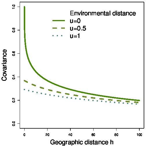
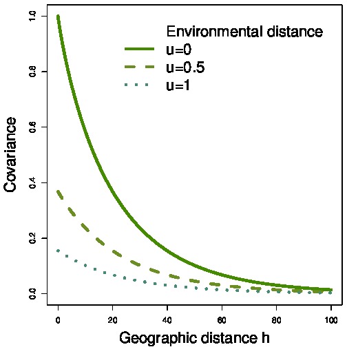
Figure 1: Cross-sections of the BRC covariance function $C(h,u)=1/\alpha_{0}\exp\left[-\left(\alpha_{G}h+\alpha_{E}u\right)^{\alpha_{2}}\right]$ with $\alpha_{0}=1$, $\alpha_{G}=1/20$ and $\alpha_{E}=2$. Left panel $\alpha_{2}=0.3$, right panel: $\alpha_{2}=0.9$.

The use of spatial covariance functions has a long tradition in statistics and the model and method proposed by Bradburd et al. (2013) can be advocated as well grounded alternative to the widely criticized partial Mantel test (Guillot & Rousset, 2013). The stable covariance and the BRC extension in particular can capture complex patterns of genetic variation, yet they depend on a small number of parameters; as such, they are potentially useful tools for modelling spatial variation in ecology and evolution. Despite its apparent simplicity, this family of covariance functions contains a subtle, but crucial, difficulty: not every function is a covariance function.
In this note, we first clarify what is involved in the specification of a covariance model and show that some of the models used earlier are not valid. Then, standing on a firm mathematical footing, we provide results on the range of validity of the models defined above and outline alternative way of constructing valid covariance models. We conclude by discussing implications of our findings for earlier works.

A covariance model must be a positive-definite function

Theoretical aspects

Considering values $y(x_{i},e_{i})$ at $n$ locations in the geographical $\times$ environmental domain, the variance of a weighted sum can be written

$$\textrm{Var}\bigg{[}\sum_{i=1}^{n}\lambda_{i}y(x_{i},e_{i})\bigg{]}=\sum_{i=1}^{n}\sum_{j=1}^{n}\lambda_{i}\lambda_{j}\textrm{Cov}[y(x_{i},e_{i}),y(x_{j},e_{j})]$$ (3)

and it is $\geqslant 0$ for any combination of weights $\lambda_{1},\ldots,\lambda_{n}$. Using a mathematical phrasing: the covariance function $\textrm{Cov}[y(x_{i},e_{i}),y(x_{j},e_{j})]$ is a positive-definite function. Consequently, if one intends to use a certain covariance function considered suitable (e.g. for modelling or computational reasons), one has to make sure that it is positive-definite, i.e. the expression in Equation (3) has to be non-negative.

A scientist using a covariance model without this property is likely to face negative variances and undefined probability densities when embedding this covariance function into a Gaussian model. This would also thwart any simulation algorithm based on the Choleski decomposition. In other words, this model would make little sense. It is therefore important to know whether the functions $C$ and $K$ defined by Equations (1-2) are valid in this respect, or in mathematical parlance: When are $C$ and $K$ positive-definite functions? This question has been overlooked so far and holds a number of subtleties, among others the fact that (i) validity in a certain dimension does not imply validity in higher dimensions, and importantly here, (ii) the answer depends on the way distances are measured (for example Euclidean in the plan vs. geodesic distance on the earth’s surface).

A worked example: spatial prediction of tree abundance data with an invalid covariance model

We illustrate some of the consequences of using an invalid covariance model on abundance data for a tree genus in the moist forest of the Congo basin. These data have been published by Mortier et al. (2013) and made publicly available via the R package SCGLR. The variable considered here consists of abundance in thousand 8km by 8 km plots. The location of sampling sites and abundance data are shown in Figure 2.

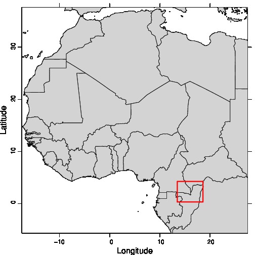
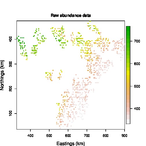
Figure 2: Study area and tree abundance data in the tropical forest of the Congo-Basin in thousand 8km$\times$8km plots.

The empirical covariance function for this variable displays a regular decrease and the exponential covariance $C(h)=\alpha_{0}^{-1}\exp(-\alpha_{G}|h|)$ provides a reasonably good fit as shown in Figure 3. Since the decrease of the empirical covariance is approximately linear, one may want to use a function of the form $C(h)=\alpha_{0}^{-1}(1-\alpha_{G}|h|)_{+}$, where $(a)_{+}$ denotes positive part of $a$, that is $C(h)=\alpha_{0}^{-1}\left(1-\alpha_{G}|h|\right)$ whenever $\quad|h|<\frac{1}{\alpha_{G}}$ and $0$ elsewhere. This covariance is known as the triangle model in the Geostatistics literature. This function provides visually an even better fit (Fig. 3).

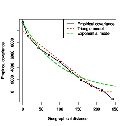
Figure 3: Empirical and theoretical covariances for the tree abundance data. Distances are in kilometers.

Unfortunately, this covariance is valid in one dimension but not in two dimensions (Chilès & Delfiner, 1999), which has consequences illustrated below. Using the exponential covariance as a covariance model for tree abundance (which is a valid model in any dimension) enables us to perform spatial prediction (Fig. 4 top left panel) and to derive an assessment of the error realized by the prediction known as kriging variance (Fig. 4 top right panel). Both maps are well behaved and seem to make sense ecologically and statistically. Using the triangle model to compute spatial prediction and kriging variance does not bring any difficulty computer-wise. The fact that the triangle function is not positive-definite shows up in the kriging variance: the latter displays spatial variation that does not mirror the location of the sampling sites, it is negative in several areas (Fig. 4 bottom right panel) and takes a minimum of $\sigma^{2}_{K}=-5720$. For short, using the triangle covariance in 2 dimensions leads to non-sensical results.

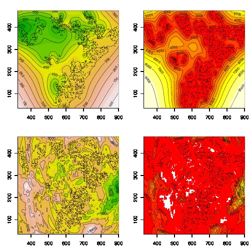
Figure 4: Spatial prediction of tree abundance data in the tropical forest of the Congo-Basin. Top: computations with an exponential covariance function. Bottom: computations with a triangular function. Left: abundance map obtained by simple kriging. Right: kriging variance (white areas in bottom right panel correspond to negative kriging variances). Eastings and Northings in kilometers.

Validity of the stable and the BRC models

In addition to $\alpha_{2}$, the models we consider involve three or four parameters. Positive-definiteness is, however, not influenced by $\alpha_{0},\alpha_{G}$ and $\alpha_{E}$ as long as they are positive. Therefore, without loss of generality on the mathematical side, we assume from now on that $\alpha_{0}=\alpha_{G}=\alpha_{E}=1$.

Euclidean distance

If $h$ is $\|x-x^{\prime}\|=\sqrt{(x_{1}-x_{1}^{\prime})^{2}+\ldots+(x_{d}-x_{d}^{\prime})^{2}}$ (the Euclidean distances in ${{\mathds{R}}^{d}}$) the stable covariance $K(h)=\exp\left[-h^{\alpha_{2}}\right]$ is a valid covariance model in ${{\mathds{R}}^{d}}$ if and only if $\alpha_{2}\in[0,2]$. Arguments proving these results are given by Schoenberg (1938).

For $u$ defined as $|e-e^{\prime}|$, the BRC model defined by $C(h,u)=\exp\left[-\left(h+u\right)^{\alpha_{2}}\right]$ is a valid covariance model on ${{\mathds{R}}^{d}}\times\mathds{R}$ if and only if $\alpha_{2}\in[0,1]$. We give a proof of this original result in the Appendix.

Geodesic distance

We denote by $\mathbb{S}^{d-1}$ the unit sphere in ${{\mathds{R}}^{d}}$ and define now $h$ as $\arccos\Big{(}\sum_{i=1}^{d}x_{i}x_{i}^{\prime}\Big{)}$ (geodesic or great circle distance on the sphere) while keeping $u=|e-e^{\prime}|$. The stable model is a valid covariance model in $\mathbb{S}^{d-1}$ if and only if $\alpha_{2}\in[0,1]$. Arguments proving this result are given by Gneiting (2013).

For the general BRC model on $\mathbb{S}^{d-1}\times\mathds{R}$, we found counter-examples showing that for $\alpha_{2}=1.001$, the model is not valid. Using a continuity argument, this means that no model with $\alpha_{2}\geqslant 1.001$ will be valid. An instance is as follows: we consider three points on the sphere with (Lon,Lat) coordinates $x_{1}=(-60.0,60)$, $x_{2}=(-60.1,60)$, $x_{3}=(-60.2,60)$ and values $e_{1}=0.1$, $e_{2}=0.2$, $e_{3}=0.3$ of an environmental variable. We also set $\alpha_{0}=1$, $\alpha_{G}=\alpha_{e}=1/300$, and $\alpha_{2}=1.01$. Under the BRC model the covariance matrix associated to this configuration is a $9\times 9$ matrix whose minimum eigenvalue is approximately $-1.84\times 10^{-5}$, which shows that the matrix is not positive-definite. A general theoretical result similar to the case of Euclidean distances is still lacking, but we conjecture that the BRC model on $\mathbb{S}^{d-1}\times\mathds{R}$ is valid if and only if $\alpha_{2}\in[0,1]$.

Other distances in the plan or the sphere

It is a common practice in ecology to measure distances in terms of cumulative cost for an individual to move from a geographical location to another. This is referred to as cost or resistance distance. There is considerable flexibility in the way such a distance can be obtained and the validity of the BRC model should be checked on a case by case basis. From the previous paragraphs, it is clear that the choice of the distance is not innocuous and that a distance that makes sense ecologically may not lead to a model that is well behaved mathematically. We note also that if the cost distance is obtained via numerical values (without a mathematical expression), there is little hope for proving the validity of a covariance model as this would involve checking all possible sums of the form given in Equation (3).

Alternate covariance models for applications in evolutionary biology

Valid gluing of the Euclidean geographical distance and the environmental distances

If the distance on ${{\mathds{R}}^{d}}\times\mathds{R}$ is defined as

$$d[(x,e),(x^{\prime},e^{\prime})]=\sqrt{\sum_{i=1}^{d}(x_{i}-x_{i}^{\prime})^{2}+(e-e^{\prime})^{2}}$$ (4)

then any valid covariance model on ${{\mathds{R}}^{d}}\times\mathds{R}$ can be used. In particular, $\exp(-d^{\;\alpha_{2}})$ is a valid model for $\alpha_{2}\in(0,2]$. See classical textbooks by Chilès & Delfiner (1999) and Diggle & Ribeiro (2007) for alternative choices. With a valid model in hands, quantifying the relative effect of distance and environment variables as suggested by Bradburd et al. (2013) can be done by re-scaling the distance as $\sqrt{\sum_{i=1}^{d}\alpha_{G}(x_{i}-x_{i}^{\prime})^{2}+\alpha_{E}(e-e^{\prime})^{2}}$.

For data gathered at large scale, one has to use geographic distances on the sphere and there seems to be no straightforward way to combine the geodesic distance with the environmental distance along this line to obtain a valid model.

Sums and products of valid models

If $C_{G}(h)$ is a valid model on ${{\mathds{R}}^{d}}$ or $\mathbb{S}^{d-1}$ and $C_{E}(u)$ is a valid model on $\mathds{R}$, then

$$C_{1}(h,u)=C_{G}(h)+C_{E}(u)$$ (5)

and

$$C_{2}(h,u)=C_{G}(h)\times C_{E}(u)$$ (6)

are valid models for which we give examples in Table 1.

Space-time covariance models

Covariance models developed to handle spatio-temporal data can be used readily for the analysis of data of the form considered by Bradburd et al. (2013). The list of such models on ${{\mathds{R}}^{d}}\times\mathds{R}$ or $\mathbb{S}^{d-1}\times\mathds{R}$ is still limited but it comes with clear guidelines about the valid range of parameters. We refer interested readers to recent spatial statistics books Gelfand et al. (2010) and Porcu et al. (2010).

Model name	Covariance function	Parameter range
Stable	$C(h)=\exp\left(-h^{\alpha}\right)$	$\alpha\in(0,2]$ on $\mathds{R}^{d}$
		$\alpha\in(0,1]$ on $\mathbb{S}^{d-1}$
BRC	$C(h,u)=\exp\left(-(h+u)^{\alpha}\right)$	$\alpha\in(0,1]$ on $\mathds{R}^{d}\times\mathds{R}$
		Unknown for $\mathbb{S}^{d-1}\times\mathds{R}$
Modified BRC	$C((x,e),(x^{\prime},e^{\prime}))=$
	$\exp\left(-\sqrt{\sum_{i=1}^{d}(x_{i}-x_{i}^{\prime})^{2}+(e-e^{\prime})^{2}}^{\;\alpha}\right)$	$\alpha\in(0,2]$ on $\mathds{R}^{d}\times\mathds{R}$
Sum of stable	$C(h,u)=\exp\left(-h^{\alpha})+\exp(-u^{\beta}\right)$	$(\alpha,\beta)\in(0,2]\times(0,2]$ on $\mathds{R}^{d}\times\mathds{R}$
models		$(\alpha,\beta)\in(0,1]\times(0,2]$ on $\mathbb{S}^{d-1}\times\mathds{R}$
Product of stable	$C(h,u)=\exp\left(-h^{\alpha})\times\exp(-u^{\beta}\right)$	$(\alpha,\beta)\in(0,2]\times(0,2]$ on $\mathds{R}^{d}\times\mathds{R}$
models		$(\alpha,\beta)\in(0,1]\times(0,2]$ on $\mathbb{S}^{d-1}\times\mathds{R}$

Table 1: Summary of covariance models with range of validity. In the table, $u$ is the environmental distance $|e-e^{\prime}|$ while $h$ refers to the Euclidean distance $\|x-x^{\prime}\|=\sqrt{\sum_{i=1}^{d}(x_{i}-x_{i}^{\prime})^{2}}$ on $\mathds{R}^{d}$, and to the geodesic distance $\arccos\Big{(}\sum_{i=1}^{d}x_{i}x_{i}^{\prime}\Big{)}$ on the unit sphere $\mathbb{S}^{d-1}$ of ${{\mathds{R}}^{d}}$.

Conclusion

There are limitations on the parameter range for the stable and the BRC models and they depend on the way distances are measured. We provide clear guidelines for the case of Euclidean distances while the case of geodesic distances still requires more work. For cost distances, a general theoretical statement is not possible and checking the validity for numerically-derived distances seems out of reach. We recommend users to be cautious when using cost distances in this context. These limitations have remained un-noticed so far and some of the earlier works making use of these models have been based on invalid parameter ranges. However, in agreement with our findings, none of these earlier studies reported empirically estimated values outside the valid ranges we establish. Our work provides some guidelines to update corresponding programs and we are happy to note that they are currently used to update the BEDASSLE computer program (G. Bradbrud, personal communication).

Funding

E.P. is funded by Proyecto Fondecyt Regular n. 1130647, M.B. by Proyecto Fondecyt Iniciación n. 11121408, G.G by Agence Nationale de la Recherche project ANR-09-BLAN-0145-01 and the Danish e-Infrastructure Cooperation.

Appendix A Appendix: valid parameter range for the BRC model

We determine here for which values of $\alpha_{2}$ the function from Equation (1) is a covariance function. A map $\gamma$ from $\mathds{R}^{d}\times\mathds{R}$ into $\mathds{R}$ is called a variogram if it represents the variance of the increments of an intrinsically stationary random field, i.e.

$$\gamma\left(x_{j}-x_{i},e_{j}-e_{i}\right)=\textrm{Var}\left(Z(x_{j},e_{j})-Z(x_{i},e_{i})\right).$$

Variograms are real-valued negative definite functions, i.e. for any finite family of points $\{(x_{i},e_{i})\}_{i=1}^{N}$ and constants $\{a_{i}\}_{i=1}^{N}$ with $\sum_{i=1}^{N}a_{i}=0$, we have

$$\sum_{i=1}^{N}\sum_{j=1}^{N}\gamma\left(x_{j}-x_{i},e_{j}-e_{i}\right)a_{i}a_{j}\leq 0.$$

The connection between variograms and covariance functions is due to Schoenberg (1938): $C:{{\mathds{R}}^{d}}\times\mathds{R}\to\mathds{R}$ is a covariance function if and only if $C(x,e)=\exp(-r\gamma(x,e))$ where $\gamma(x,e)$ is a variogram.

Thus, we can re-cast the question about the valid range of parameter in the following way:

for which $$\alpha_{2}>0 (h,u)\mapsto\left(h+u\right)^{\alpha_{2}}$$ is the function a variogram? (7)

As before, $h=\|x\|=\sqrt{x_{1}^{2}+\ldots+x_{d}^{2}}$ is the Euclidean distance (taken from the origin) in ${{\mathds{R}}^{d}}$ and $u=|e|$ is the ecological distance (in $\mathds{R}$, also relative to the origin). In order to simplify the notation, we write $\alpha$ instead of $\alpha_{2}$.

It is known that every continuous variogram on ${{\mathds{R}}^{n}}$ is given by a Lévy–Khintchine formula:

$$\gamma(\eta)=\frac{1}{2}\eta\cdot Q\eta+\int_{y\neq 0}\Big{(}1-\cos\Big{(}{\textstyle\sum\limits_{i=1}^{n}\eta_{i}y_{i}}\Big{)}\Big{)}\,\nu(dy),\quad\eta\in{{\mathds{R}}^{n}},$$ (8)

where $Q$ is a symmetric positive semi-definite $n\times n$ matrix, and $\nu$ is a measure on ${{\mathds{R}}^{n}}\setminus\{0\}$ such that $\int_{y\neq 0}\|y\|^{2}/(1+\|y\|^{2})\,\nu(dy)<\infty$; $\gamma$ is uniquely determined by $(Q,\nu)$ and vice versa. Typical examples of continuous variograms on ${{\mathds{R}}^{n}}$ are

$$\|\eta\|^{2},\quad\eta\cdot Q\eta,\quad 1-\cos y\cdot\eta,\quad\log(1+\|\eta\|^{2}),\quad\|\eta\|^{\alpha}\;(0<\alpha<2).$$

A good source for variograms (which are also known as negative definite real functions) are the monographs by Berg & Forst (1975) and R.L. Schilling & Vondraček (2012). We only need the following properties.

(A)

Subadditivity: If $\gamma(\eta)$ is a continuous variogram, then $\sqrt{\gamma(\eta+\eta)}\leqslant\sqrt{\gamma(\eta)}+\sqrt{\gamma(\eta)}$. In particular, $\gamma(\eta)$ grows at most like $\|\eta\|^{2}$ as $\|\eta\|\to\infty$.

(B)

Closure under pointwise limits: If $\gamma_{j}(\eta),j=1,2,\ldots$ are continuous variograms such that the limit $\gamma(\eta):=\lim_{j\to\infty}\gamma_{j}(\eta)$ exists and is continuous, then $\gamma(\eta)$ is a continuous variogram.

(C)

Let $\eta\mapsto\gamma(\eta)$ be a continuous variogram on $\mathds{R}^{d}$ and write $\eta=(\eta^{\prime},\eta^{\prime\prime})$ where $\eta^{\prime}\in{{\mathds{R}}^{n}}$, $\eta^{\prime\prime}\in\mathds{R}^{d-n}$. Then $\eta^{\prime}\mapsto\gamma(\eta^{\prime},0)$ is a continuous variogram on ${{\mathds{R}}^{n}}$.

(D)

Let $\gamma(\eta^{\prime})$, $\psi(\eta^{\prime\prime})$ be continuous variograms on ${{\mathds{R}}^{n}}$ and $\mathds{R}^{m}$, respectively. Then $(\eta^{\prime},\eta^{\prime\prime})\mapsto\gamma(\eta^{\prime})+\psi(\eta^{\prime\prime})$ is a continuous variogram on ${{\mathds{R}}^{d}}=\mathds{R}^{n+m}$.

The variogram property is also preserved under a technique called Bochner’s subordination, cf. R.L. Schilling & Vondraček (2012). At the level of the random variables this corresponds to a mixture of the processes with a further infinitely divisible random variable, at the level of variograms this is just a composition with the class of so-called Bernstein functions. These are also given by a Lévy–Khintchine formula

$$f(\lambda)=b\lambda+\int_{0+}^{\infty}(1-e^{-s\lambda})\,\mu(ds),\quad\lambda\geqslant 0,$$

where $b\geqslant 0$ and $\mu$ is a measure on $(0,\infty)$ such that $\int_{0}^{\infty}s(1+s)^{-1}\,\mu(ds)<\infty$. Typical examples of Bernstein functions are

$$\lambda,\quad\lambda^{\alpha}\;(0<\alpha<1),\quad\log(1+\lambda).$$

Theorem 1.

If $\gamma(\eta)$ is a continuous variogram and $f$ is a Bernstein function, then $f(\gamma(\eta))$ is again a continuous variogram.

We now have all ingredients for the

Proof of the valid parameter range.

Note that $\psi(\eta)=\|\eta\|=\sqrt{\eta_{1}^{2}+\ldots+\eta_{d}^{2}}$ and $\phi(\tau)=|\tau|$ are continuous variograms in $\mathds{R}^{d}$ and $\mathds{R}$, respectively. Moreover, take the Bernstein function $f(\lambda)=\lambda^{\alpha}$, $\lambda>0$; the corresponding mixing random variables are one-sided $\alpha$-stable random variables (if $0<\alpha<1$) or a deterministic drift (if $\alpha=1$). By property (D) and subordination,

$$(\eta,\tau)\mapsto\gamma_{\alpha}(\eta,\tau):=(\|\eta\|+|\tau|)^{\alpha},\quad 0<\alpha\leqslant 1,$$ (9)

is a continuous variogram.

On the other hand, by the quadratic growth property, see (A), it is clear that $\gamma_{\alpha}(\eta,\tau)$ is not a variogram if $\alpha>2$.

Let us now consider the case where $\alpha\in(1,2]$. Assume first that $\alpha=2$. Then

$$(\|\eta\|+|\tau|)^{2}=\|\eta\|^{2}+2\,\|\eta\|\cdot|\tau|+\tau^{2}.$$

Since $\|\eta\|^{2}+\tau^{2}$ would appear in the Lévy–Khintchine formula (8) as part of the expression involving the matrix $Q$, it is enough to prove or disprove that the mixed term $c(\eta,\tau):=\|\eta\|\cdot|\tau|$ is a continuous variogram. But

$$\sqrt{\|\eta\|\cdot|\tau|}=\sqrt{c(\eta,\tau)}\geqslant\sqrt{c(\eta,0)}+\sqrt{c(0,\tau)}=0,$$

which means that $\sqrt{c(\eta,\tau)}$ is not sub-additive, violating the subadditivity property (A), i.e.

$$(\eta,\tau)\mapsto(\|\eta\|+|\tau|)^{2}\quad\text{is not a variogram}.$$

Now we use the property (B): Clearly, $\lim_{j\to\infty}(\|\eta\|+|\tau|)^{2-1/j}=(\|\eta\|+|\tau|)^{2}$. Since variograms are preserved under pointwise limits, we conclude from this, and the subordination argument, that there is some $1\leqslant b<2$ such that

$$(\eta,\tau)\mapsto(\|\eta\|+|\tau|)^{\alpha}\quad\text{is\ \ }\begin{cases}\text{\ a continuous variogram if}&0<\alpha\leqslant b\\ \text{\ not a continuous variogram if}&\alpha>b.\end{cases}$$

We conclude the proof by showing that necessarily $b=1$. Use Property (C) above, and suppose that the function in Equation (9) is a variogram on $\mathds{R}^{d}$. Then the function

$$\tilde{\gamma}(\eta_{1},\tau):=\gamma_{\alpha}\left((\eta_{1},0,\ldots,0),\tau\right)$$

is a variogram on $\mathds{R}\times\mathds{R}$. Arguments by Zastavnyi (2000) show that this is true if and only if $\alpha\leq 1$, which completes the proof. ∎

References

- Berg & Forst (1975) Berg, C. & Forst, G. (1975). Potential Theory on Locally Compact Abelian Groups. Springer, Berlin.
- Bradburd et al. (2013) Bradburd, G., Ralph, P. & Coop, G. M. (2013). Disentangling the effects of geographic and ecological isolation on genetic differentiation. Evolution, doi:10.1111/evo.12193.
- Chilès & Delfiner (1999) Chilès, J. & Delfiner, P. (1999). Geostatistics: Modeling Spatial Uncertainty. Wiley, Hoboken, NJ, USA.
- Diggle & Ribeiro (2007) Diggle, P. & Ribeiro, P. (2007). Model-based geostatistics. Spinger, New York.
- Diggle et al. (2007) Diggle, P. J., Thomson, M. C., Christensen, O. F., Rowlingson, B., , Obsomer, V., Gardon, J., Wanji, S., Takougang, I., Enyong, P., Kamgno, J., Remme, J. H., Boussinesq, M. & Molyneux, D. H. (2007). Spatial modelling and the prediction of Loa loa risk: decision making under uncertainty. Annals of Tropical Medicine and Parasitology, 6, 499–509.
- Diniz-Filho et al. (2003) Diniz-Filho, J., Bini, L. & Hawkins, B. (2003). Spatial autocorrelation and red herrings in geographical ecology. Global Ecology and Biogeography, 12, 53–64.
- Gelfand et al. (2010) Gelfand, A. E., Diggle, P., Guttorp, P. & Fuentes, M., eds. (2010). Handbook of Spatial Statistics. Handbooks of Modern Statistical Methods. Chapman & Hall/CRC.
- Gneiting (2013) Gneiting, T. (2013). Strictly and Non-Strictly Positive Definite Functions on Spheres. Bernoulli. To appear.
- Guillot & Rousset (2013) Guillot, G. & Rousset, F. (2013). Dismantling the Mantel tests. Methods in Ecology and Evolution, 4, 336–344.
- Guillot & Santos (2009) Guillot, G. & Santos, F. (2009). A computer program to simulate multilocus genotype data with spatially auto-correlated allele frequencies. Molecular Ecology Resources, 9, 1112 – 1120.
- Hay et al. (2009) Hay, S. I., Guerra, C. A., Gething, P. W., Patil, A. P., Tatem, A. J., Noor, A. M., Kabaria, C. W., Manh, B. H., Elyazar, I. R., Brooker, S. et al. (2009). A world malaria map: Plasmodium falciparum endemicity in 2007. PLoS medicine, 6, e1000048.
- Jackson & Caldwell (1993) Jackson, R. & Caldwell, M. (1993). Geostatistical patterns of soil heterogeneity around individual perennial plants. Journal of Ecology, pp. 683–692.
- Levin (1992) Levin, S. A. (1992). The problem of pattern and scale in ecology: the Robert H. MacArthur award lecture. Ecology, 73, 1943–1967.
- Liebhold et al. (1993) Liebhold, A. M., Rossi, R. E. & Kemp, W. P. (1993). Geostatistics and geographic information systems in applied insect ecology. Annual Review of Entomology, 38, 303–327.
- Mortier et al. (2013) Mortier, F., Trottier, C., Cornu, G. & Bry, X. (2013). SCGLR - An R Package for Supervised Component Generalized Linear Regression. Journal of Statistical Software. Submitted.
- Novembre & Stephens (2008) Novembre, J. & Stephens, M. (2008). Interpreting principal component analyses of spatial population genetic variation. Nature Genetics, 40, 646–649.
- Perry et al. (2002) Perry, J., Liebhold, A., Rosenberg, M., Dungan, J., Miriti, M., Jakomulska, A. & Citron-Pousty, S. (2002). Illustrations and guidelines for selecting statistical methods for quantifying spatial pattern in ecological data. Ecography, 25, 578–600.
- Porcu et al. (2010) Porcu, E., Montero, J. & Schlather, M., eds. (2010). Advances and Challenges in Space-time Modelling of Natural Events. Springer, Heidelberg Dordrecht London New York.
- Rahbek et al. (2007) Rahbek, C., Gotelli, N. J., Colwell, R. K., Entsminger, G. L., Rangel, T. F. L. & Graves, G. R. (2007). Predicting continental-scale patterns of bird species richness with spatially explicit models. Proceedings of the Royal Society B: Biological Sciences, 274, 165–174.
- R.L. Schilling & Vondraček (2012) R.L. Schilling, R. S. & Vondraček, Z. (2012). Bernstein Functions: Theory and Applications. De Gruyter, Berlin. (2nd ed).
- Robertson (1987) Robertson, G. P. (1987). Geostatistics in ecology: interpolating with known variance. Ecology, 68, 744–748.
- Rundel et al. (2013) Rundel, C., Wunder, M., Alvarado, A., Ruegg, K., Harrigan, R., Schuh, A., Kelly, J. F., Siegel, R. B., DeSante, D., Smith, T. B. & Novembre, J. (2013). Novel statistical methods for integrating genetic and stable isotope data to infer individual-level migratory connectivity. Molecular ecology, 16, 4163–76.
- Schoenberg (1938) Schoenberg, I. J. (1938). Metric Spaces and Completely Monotone Functions. Annals of Mathematics, 39, 811–841.
- Wasser et al. (2007) Wasser, S., Mailand, C., Booth, R., Mutayoba, B., Kisamo, E. & Stephens, M. (2007). Using DNA to track the origin of the largest ivory seizure since the 1989 trade ban. Proceedings of the National Academy of Sciences, 104, 4228–4233.
- Wasser et al. (2004) Wasser, S., Shedlock, A., Comstock, K., Ostrander, E., Mutayoba, B. & Stephens, M. (2004). Assigning African elephants DNA to geographic region of origin: applications to the ivory trade. Proceedings of the National Academy of Sciences, 101, 14847–14852.
- Zastavnyi (2000) Zastavnyi, V. (2000). On Positive Definiteness of Some Functions. Journal of Multivariate Analysis, pp. 55–81.