Quantum probes for the spectral properties of a classical environment

Abstract

We address the use of simple quantum probes for the spectral characterization of classical noisy environments. In our scheme a qubit interacts with a classical stochastic field describing environmental noise and is then measured after a given interaction time in order to estimate the characteristic parameters of the noise. In particular, we address estimation of the spectral parameters of two relevant kinds of non-Gaussian noise: random telegraph noise with Lorentzian spectrum and colored noise with $1/f^{\alpha}$ spectrum. We analyze in details the estimation precision achievable by quantum probes and prove that population measurement on the qubit is optimal for noise estimation in both cases. We also evaluate the optimal interaction times for the quantum probe, i.e. the values maximizing the quantum Fisher information (QFI) and the quantum signal-to-noise ratio. For random telegraph noise the QFI is inversely proportional to the square of the switching rate, meaning that the quantum signal-to-noise ratio is constant and thus the switching rate may be uniformly estimated with the same precision in its whole range of variation. For colored noise, the precision achievable in the estimation of “color”, i.e. of the exponent $\alpha$, strongly depends on the structure of the environment, i.e. on the number of fluctuators describing the classical environment. For an environment modeled by a single random fluctuator estimation is more precise for pink noise, i.e. for $\alpha=1$, whereas by increasing the number of fluctuators, the quantum signal-to-noise ratio has two local maxima, with the largest one drifting towards $\alpha=2$, i.e. brown noise.

In any communication channel or measurement scheme, the interaction of the information carriers with the external environment introduces noise in the system, thus degrading the overall performances. The precise characterization of the noise is thus a crucial ingredient for the design of high-precision measurements and reliable communication protocols. In many physical situations, the main source of noise is associated to the fluctuations of bistable quantities. In these cases, a suitable description of the noise is given in terms of classical stochastic processes band13 ; berman12 ; galp06 . In particular, in the case of phase damping, i.e. pure dephasing, it has been shown that the interaction of a quantum system with a quantum bath can be written in terms of a random unitary evolution driven by a classical stochastic process joynt13 ; helm11 .

The characterization of classical noise is often performed by collecting a series of measurements to estimate the autocorrelation function and the spectral properties hur51 ; per03 ; barunik10 ; kend99 ; salomon13 ; magd13 . This procedure is generally time consuming and may require the control of a complex system. A question thus arises on whether more effective techniques may be developed. To this purpose, we address the use of quantum probes to estimate the parameters of classical noise. We assume to have a quantum system interacting with the classical fluctuating field generating the noise and explore the performances of quantum measurements performed at a fixed interaction time to extract information about the classical noise. The power and implications of this idea are undeniable: the features of a complex system may be determined by monitoring a small probe, which is usually characterized by few and easily controllable degrees of freedom. The simplest and paradigmatic example of this situation is that of a qubit interacting with a noisy environment. After a given interaction time, which may be suitably optimized, quantum-limited measurements on the qubit may be used to characterize the environment, e.g. to estimate the parameters describing its noise spectrum.

In this paper we focus on the characterization of two classes of classical noise: random telegraph noise (RTN) with Lorentzian spectrum and the power-law $1/f^{\alpha}$ colored spectra arising from the interaction with a collection of random bistable fluctuators. Both RTN and colored noise are examples of classical non-Gaussian noise occurring in several system of interest. Indeed, the microscopic models underlying these kinds of noise have been extensively analyzed in the literature galperin ; benIJ ; bordonefnl ; weissman ; paladinorev ; benedettipra ; bus13 . The relevant parameters characterizing this kinds of noise are the switching rate of the RTN and the exponent $\alpha$ in the case of power-law spectra. Both quantities do not correspond to observables in a strict sense and therefore we have to resort to indirect measurements performed on the quantum probe to infer their value. In order to optimize this inference procedure we employ tools from local quantum estimation theory hel76 ; mal93 ; brau94 ; brody99 ; paris09 ; esch12 , which have already been proved useful in the estimation of static noise parameters hotta05 ; monras07 ; fuj01 ; ji08 ; dau06 and in several other scenarios, as for example the estimation of quantum correlations brida2010 ; brida2011 ; blandino2012 ; benedetti2013 , Gaussian states mon10 ; pinel13 ; monar , optical phase monras06 ; kac10 ; cable10 ; durk10 ; genoni2011 ; spagnolo2012 , critical systems zan08 ; inver08 and quantum thermometry brunelli2011 . In particular, we will optimize the initial preparation of the qubit and the interaction time in order to maximize the quantum Fisher information and the quantum signal-to-noise ratio. Furthermore, we show that population measurement provides optimal inference for both the noise models.

This paper is organized as follows: in Section I we introduce the physical dephasing model employed throughout the paper and describe the main features of RTN and colored noise. In Section II we briefly review the main tools of quantum estimation theory, whereas in Section III we present our results on the precision achievable by quantum probes in the estimation of the spectral properties of noisy random environments. Section IV closes the paper with concluding remarks.

I The Physical Model

In order to gain information about a complex environment, we analyze its influence on the dynamics of a quantized information carrier. In the simplest case this corresponds to a qubit interacting with a classical stochastic field. Two different field spectra will be considered: the Lorentzian spectrum generated by a random telegraph noise and the $1/f^{\alpha}$ colored spectrum stemming from a collection of random bistable fluctuators. In both cases the noise induced by the classical field is described by a non-Gaussian process, meaning that the sole knowledge of the second-order statistics is not sufficient to fully characterize the process.

We focus attention on situations where the dominant process induced by the environmental noise is pure dephasing. This corresponds to have the quantum probe, a qubit, coupled to a classical field in a given direction, say $x$. The Hamiltonian of the qubit thus reads

$$\mathcal{H}(t)=\epsilon\;\mathbb{I}+\nu\,c(t)\,\sigma_{x},$$ (1)

where $\epsilon$ is the energy of the qubit eigenstates assumed to be degenerate, $c(t)$ is the stochastic non-Gaussian process, $\sigma_{x}$ is the Pauli matrix, $\nu$ describes the coupling strength with the environment and $\hbar$ was set to 1. We also assume that the qubit is initially prepared in a generic pure state

$$|\psi_{0}\rangle=\cos\frac{\theta}{2}\,|0\rangle+e^{i\phi}\sin\frac{\theta}{2}\,|1\rangle.$$ (2)

Upon studying the dynamics of the qubit subject to noise we gain information about the spectral properties of the environment.

I.1 Random telegraph noise

Random telegraph noise describes the fluctuations induced by the interaction with a classical bistable fluctuator, i.e. a physical system which flips between two given configurations with a fixed switching rate. RTN is characterized by an exponential autocorrelation function and a Lorentzian power spectrum. In mathematical terms, RTN corresponds to an interaction Hamiltonian as in Eq. (1) with $c(t)$ flipping between the values $c(t)=\pm 1$ at a switching rate $\xi$.

Hereafter we work with dimensionless quantities by scaling the time and the switching rate in unit of $\nu$. In particular, we substitute $t\rightarrow\tau=\nu t$ and $\xi\rightarrow\gamma=\xi/\nu$.

The density matrix of a qubit interacting with a RTN classical environment is obtained averaging the unitary evolved state over all possible temporal sequences of the stochastic process $c(t)$ benedetti1 ; paladino ; abel :

$$\rho(\tau,\gamma,\theta,\phi)=\langle U(\tau)\rho_{0}U^{\dagger}(\tau)\rangle_{c(t)}$$ (3)

where $U(\tau)=e^{-i\int_{0}^{\tau}{\mathcal{H}}(s)ds}$ is the evolution operator, $\rho_{0}=|\psi_{0}\rangle\langle\psi_{0}|$ is the initial density matrix, and $\langle\dots\rangle_{c(t)}$ denotes average over the process. The density matrix in the computational basis $\{|0\rangle,|1\rangle\}$ reads:

$$\rho(\tau,\gamma, \theta,\phi)=$$

$$\frac{1}{2}(\cos\theta\,\mathbb{I}+D(\tau,\gamma)\,\sigma_{z}+$$

$$\sin\theta\,\cos\phi\,\sigma_{x}-\sin\theta\,\sin\phi\,D(\tau,\gamma)\,\sigma_{y})$$ (4)

with

$$D(\tau,\gamma) \equiv\langle\text{exp}\left[-i\int_{0}^{\tau}c(s)\,ds\right]\rangle_{c(t)}$$

$$=e^{-\gamma\tau}\left(\cosh\delta\tau+\frac{\gamma\sinh\delta\tau}{\delta}\right)$$ (5)

and where $\delta\equiv\delta(\gamma)=\sqrt{\gamma^{2}-4}$. For $\gamma<2$, $D(\tau,\gamma)$ is a damped oscillating function of time, while for $\gamma\geq 2$ $D(\tau,\gamma)$ decays monotonically in time. The first case is often referred to as slow RTN and corresponds to a non-Markovian map bpm13 , while the second is called fast RTN and leads to a Markovian dynamics.

I.2 Colored noise

A complex environment characterized by a noise spectrum of the form $1/f^{\alpha}$ in a given frequency range $[\gamma_{1},\gamma_{2}]$, correspond to a collection of one or more bistable fluctuators whose switching rates assume random values $f\in[\gamma_{1},\gamma_{2}]$ according to the probability distribution

$$p_{\alpha}(\gamma)=\left\{\begin{array}[]{ll}\frac{1}{\gamma\,\ln(\gamma_{2}/\gamma_{1})}&\alpha=1\\ &\\ \frac{\alpha-1}{\gamma^{\alpha}}\left[\frac{(\gamma_{1}\gamma_{2})^{\alpha-1}}{\gamma_{2}^{\alpha-1}-\gamma_{1}^{\alpha-1}}\right]&\alpha\neq 1\end{array}\right.$$ (9)

We assume colored noise with $\alpha<2$ and, in particular, focus attention on classical noise with exponent in the range $\alpha\in[1/2,2]$. The case $\alpha=1$ is usually referred to as pink noise and the case $\alpha=2$ as Brown(ian) noise.

For colored noise the field $c(t)$ in Eq. (1) is a superposition of $N$ random bistable fluctuators $c(t)=\sum_{j=1}^{N}c_{j}(t)$, where the $c_{j}(t)$ are classical stochastic fields describing independent RTN sources with random switching rates extracted from the distribution (9). The density matrix of a qubit interacting with colored noise is obtained as the average over all the environmental degrees of freedom benedettipra :

$$\rho(\tau,\alpha,\theta,\phi)=\int_{\gamma_{1}}^{\gamma_{2}}\!\!\rho(\tau,\gamma,\theta,\phi)\;p_{\alpha}(\gamma)\;d\gamma$$ (10)

where $\rho(\tau,\gamma,\theta,\phi)$ is the expression of Eq. (3) with the average taken over the global field $c(t)$. Eq. (10) my be re-written as:

$$\rho(\tau,\alpha, \theta,\phi)=$$

$$\frac{1}{2}(\cos\theta\,\mathbb{I}+\Lambda(\tau,\alpha,N)\,\sigma_{z}+$$

$$\sin\theta\,\cos\phi\,\sigma_{x}-\sin\theta\,\sin\phi\,\Lambda(\tau,\alpha,N)\,\sigma_{y})$$ (11)

where $N$ is the number of fluctuators, $\Lambda(\tau,\alpha,N)=\left[\Lambda(\tau,\alpha)\right]^{N}$, and

$$\Lambda(\tau,\alpha)=\int_{\gamma_{1}}^{\gamma_{2}}\!\!p_{\alpha}(\gamma)D(\tau,\gamma)d\gamma\,.$$ (12)

The dynamics of the qubit is governed by the function $\Lambda$, which can be easily evaluated numerically, either by numerical integration of Eq. (12) or by the equivalent series representation reported in Appendix A.

II Local quantum estimation theory

In this section we review the main tools of local QET. Let us consider a family of quantum states $\rho_{\lambda}$ depending on a parameter $\lambda$. We are interested in inferring the value of the parameter and to this aim we perform repeated measurements on the system and then process the overall sample of outcomes. An estimator $\bar{\lambda}=\bar{\lambda}(x_{1},x_{2}\dots x_{M})$ is a function of the outcomes $\{x_{i}\}$ and we denote by $V(\bar{\lambda})$ the corresponding mean square error. The smaller is $V(\bar{\lambda})$, the more precise the estimator is. In fact, there is a bound to the precision of any unbiased estimator, given by the Cramer-Rao (CR) inequality:

$$V(\bar{\lambda})\geq\frac{1}{M\,F(\lambda)}$$ (13)

where $M$ is the number of measurements and $F(\lambda)$ is the Fisher information:

$$F(\lambda)=\int\!\!dx\,p(x|\lambda)\,\left[\partial_{\lambda}\log p(x|\lambda)\right]^{2},$$ (14)

where $p(x|\lambda)$ is the conditional probability of obtaining the outcome $x$ when the true value of the parameter is $\lambda$. In the case of a qubit, we may for instance consider the population measurement. The Fisher is given by:

$$F(\lambda)=\frac{(\partial_{\lambda}\rho_{00})^{2}}{\rho_{00}}+\frac{(\partial_{\lambda}\rho_{11})^{2}}{\rho_{11}}$$ (15)

where $\rho_{ii}$ are the two diagonal elements of the density matrix in the population basis. In order to compute the ultimate bound to precision as posed by quantum mechanics, the FI must be maximized over all possible measurements. Upon introducing the Symmetric Logarithmic Derivative $L_{\lambda}$ as the operator which satisfies the relation:

$$\frac{L_{\lambda}\rho_{\lambda}+\rho_{\lambda}L_{\lambda}}{2}=\partial_{\lambda}\rho_{\lambda}$$ (16)

the quantum CR bound is found:

$$V(\lambda)\geq\frac{1}{M\,H(\lambda)}.$$ (17)

Here $H(\lambda)=\text{Tr}[\rho_{\lambda}L_{\lambda}^{2}]$ is the so-called quantum Fisher information. In the case of a qubit, the expression of the QFI can be found after diagonalizing the density matrix $\rho_{\lambda}=\sum_{n=1}^{2}\rho_{n}|\phi_{n}\rangle\langle\phi_{n}|$:

$$H(\lambda)=\sum_{n=1}^{2}\frac{(\partial_{\lambda}\rho_{n})^{2}}{\rho_{n}}+2\sum_{n\neq m}\frac{(\rho_{n}-\rho_{m})^{2}}{\rho_{n}+\rho_{m}}|\langle\phi_{m}|\partial_{\lambda}\phi_{n}\rangle|^{2}.$$ (18)

The first term in Eq. (18) is the classical FI of the distribution $\{\rho_{n}\}$, while the second term has a quantum nature and vanishes when the eigenvectors of $\rho_{\lambda}$ do not depend upon the parameter $\lambda$. When the condition $F(\lambda)=H(\lambda)$ is fulfilled, the measurement is said to be optimal. If equality in Eq. (13) is satisfied the corresponding estimator is said to be efficient.

A global measure of the estimability of a parameter is given by the single-measurement signal-to-noise ratio ${\rm SNR}=\lambda^{2}/V(\lambda)$. Using the Cramer-Rao bound we have that the SNR is bounded by the so-called quantum signal-to-noise ratio ${\rm QSNR}$ $R=\lambda^{2}H(\lambda)$, which represents the ultimate quantum bound to the estimability of a parameter.

III Parameter estimation by quantum probes

The goal of an estimation procedure is not only to determine the value of an unknown parameter, but also to infer this value with the largest possible precision. The quantum CR inequality set a bound to the ultimate precision that can be achieved in estimating a parameter and, in turn, on the corresponding signal-to-noise ratio.

In this section we discuss optimization of parameter estimation by quantum probes. In other words, we determine the initial qubit preparation and the interaction time that maximize the QFI, and show that the corresponding ultimate precision may be achieved by population measurement on the qubit. We then discuss in detail under which conditions it is possible to estimate efficiently the spectral properties of the environmental noise.

Let us start by considering a generic pure dephasing model

$$\rho=\frac{1+\Gamma(\lambda)}{2}\rho_{0}+\frac{1-\Gamma(\lambda)}{2}\sigma_{x}\rho_{0}\sigma_{x}$$ (19)

where $\Gamma(\lambda)$ is a real coefficient taking both negative and positive values between $\pm 1$. If we set $\phi=0$ in Eq. (2), the QFI can be analytically computed and it takes the expression:

$$H(\lambda)=\cos^{2}(\theta)\;\frac{\big{[}\partial_{\lambda}\Gamma(\lambda)\big{]}^{2}}{1-\Gamma^{2}(\lambda)}.$$ (20)

As it is apparent from Eq. (20) the QFI is maximized for $\theta=0$. In this case the optimal initial state preparation is the state $|\psi\rangle=|0\rangle$. If we consider the most general initial state (2) with $\phi\neq 0$, we have numerical evidence that the QFI is still maximized by the state $|0\rangle$ for any choice of $\Gamma(\lambda)$.

III.1 Random telegraph noise

In the case of a RTN the parameter to be estimated is the switching rate $\gamma$. Starting from the qubit prepared in the state $|0\rangle$ and using Eq. (4), the family of possible evolved states may be written as

$$\rho(\tau,\gamma)=\frac{1}{2}\left(\begin{array}[]{cc}1+D(\tau,\gamma)&0\\ 0&1-D(\tau,\gamma)\\ \end{array}\right).$$ (23)

We know that the optimal measurement is a projective one barn00 ; luati . Besides, the eigenvectors of the matrix (23) do not depend on the parameter $\gamma$ and the second term in Eq. (18) vanishes. Looking at the very form of the matrices in Eq. (23) one immediately recognizes that the QFI coincides with the FI of population measurement and can be written as:

$$H(\tau,\gamma)=\frac{[\partial_{\gamma}D(\tau,\gamma)]^{2}}{1-D(\tau,\gamma)^{2}},$$ (24)

which is the analogue of Eq. (20) with the coefficient $\Gamma(\lambda)$ replaced by coefficient $D(\tau,\gamma)$. The two different regimes of slow and fast RTN give rise to different behaviors for the QFI, which are illustrated in Fig. 1. For slow RTN $H$ is shown in the upper panel of Fig. 1: the QFI is characterized by an oscillating behavior and, in particular, for $\gamma\ll 2$ the peaks are located at multiples of $\tau=\frac{\pi}{2}$. In the fast RTN case (see the lower panel of Fig. 1), $H$ has only one peak and its maximum value decreases with $\gamma$.

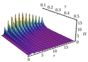
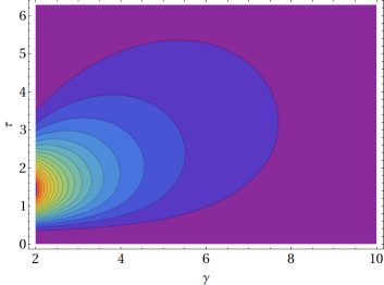
Figure 1: (Color online): The upper panel shows the QFI $H(\tau,\gamma)$ as a function of the interaction time $\tau$ and the switching rate $\gamma$ for slow RTN. The lower panel shows a contour plot of of $H(\tau,\gamma)$ for fast RTN.

In order to optimize the inference procedure we look for the interaction time that maximizes the QFI $H(\tau,\gamma)$ (and, in turn, the QSNR $R$) at each fixed value of the switching rate $\gamma$. The maximization of the QFI has been performed numerically, leading to the following approximation

$$\tau_{{\rm opt}}(\gamma)\simeq\left\{\begin{array}[]{cc}\text{nint}\left[\frac{1}{2\gamma}\right]\frac{\pi}{2}&\quad\gamma<2\\ &\\ \frac{2}{5}\gamma&\quad\gamma>2\end{array}.\right.$$ (25)

The approximation is very good for $\gamma$ in range [$10^{-3},10^{3}$] except for $\gamma\simeq 2$ where the peaks are not exactly located at multiples of $\tau=\frac{\pi}{2}$ and Eq. (25) is valid only to a first approximation. In order to further illustrate the behavior of the QFI in the slow RTN regime, in Fig. 2 we show the optimal interaction time $\tau_{{\rm opt}}$ as a function of the switching rate. The step-like behavior of $\tau_{{\rm opt}}$ is due to the oscillating behavior of the QFI. On the other hand, in the fast RTN regime, the maximum moves continuously as a function of $\gamma$.

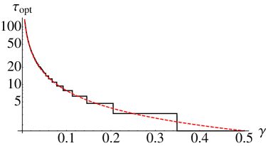
Figure 2: (Color online): The optimal interaction time $\tau_{{\rm opt}}$, maximizing the quantum Fisher information $H(\tau,\gamma)$ for slow RTN, as a function of the switching rate $\gamma$ (black line). The dashed red curve denotes the function $\pi/4\gamma$.

As seen from Eq. (25), optimal times increase with decreasing $\gamma$ in the slow RTN regime and with increasing $\gamma$ in the fast RTN regime. When small switching rates are considered, long times are necessary to see the effect of the environment on the probe, in agreement with the non Markovian character of the corresponding evolution map Sun10 ; bpm13 . In the case $\gamma\gg 2$, the qubit and the external fluctuators act as if they were decoupled, so long observation times are required to see the influence of the external noise on the dynamics of the qubit. In both cases, the maximum values $H(\tau_{{\rm opt}},\gamma)$ of the QFI are inversely proportional to $\gamma^{2}$. In particular, a numerical fit in range [$10^{-3},10^{3}$] leads to

$$H(\gamma)\approx\frac{a}{\gamma^{2}}.$$ (26)

where $a$ is of the order of 0.1. The quantum signal-to-noise ratio ${\rm QSNR}=\gamma^{2}H(\gamma)\simeq a$ is thus constant, meaning that quantum probes allow one for a uniform estimation of the switching rate in the whole range of values we have considered.

III.2 Colored noise

In the case of a collection of random bistable fluctuators, the relevant parameter to be estimated is the “color” of the noise, i.e. the exponent $\alpha$. Following the general arguments mentioned at the beginning of this Section we assume that the probe qubit is initially prepared in the state $|0\rangle$. Its time evolution is thus described by the density matrix:

$$\rho(\tau,\alpha,N)=\frac{1}{2}\left(\begin{array}[]{cc}1+\Lambda(\tau,\alpha,N)&0\\ 0&1-\Lambda(\tau,\alpha,N)\\ \end{array}\right).$$ (29)

Also for colored noise the eigenvectors do not depend on the parameter $\alpha$ and thus the FI for population measurement coincides with the QFI, which is given by

$$H(\tau,\alpha,N)=N^{2}\;\frac{\Lambda(\tau,\alpha)^{2N-2}\,}{1-\Lambda(\tau,\alpha)^{2N}}\Big{[}\partial_{\alpha}\Lambda(t,{\alpha})\Big{]}^{2}\,.$$ (30)

For colored environment realized by a single random fluctuator the above formula reduces to

$$H(\tau,\alpha)=\frac{\big{[}\partial_{\alpha}\Lambda(\tau,\alpha)\big{]}^{2}}{1-\Lambda(\tau,\alpha)^{2}}\,.$$ (31)

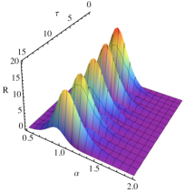
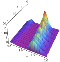
Figure 3: (Color online) Spectral characterization of colored noise: The left panel shows the QSNR $R(\tau,\alpha,N)$ as a function of the interaction time and the exponent $\alpha$ for a single fluctuator $N=1$. The right panel shows the same quantity for $N=10$.

The QFI depends on the interaction time $\tau$, the exponent $\alpha$ and the number of fluctuators $N$. Different values for $\alpha$ and $N$ may lead to considerably different temporal behaviors for the QFI. This is illustrated in Fig. 3, where we show the QSNR $R(\tau,\alpha,N)=\alpha^{2}H(\tau,\alpha,N)$ as a function of $\alpha$ and $\tau$ for two different numbers of fluctuators. When a single fluctuator is considered, the QSNR has a maximum located at $\alpha=1$, which corresponds to the best estimable value for the parameter. The situation is totally reversed in the case of $N=10$ fluctuators, where values of $\alpha$ close to one correspond to a very low QSNR.

In order to further illustrate this behavior, in Fig. 4 we show the QSNR, already maximized over the interaction time, as a function of $\alpha$ for (three) fixed numbers of fluctuators. For a single fluctuator the QSNR exhibits a single maximum located at $\alpha=1$, i.e. pink noise is more precisely estimable than other kind of noise. On the other hand, when the number of fluctuators increases, two maxima appear and their location move away from $\alpha=1$ for increasing $N$, with the largest maximum drifting towards $\alpha=2$.

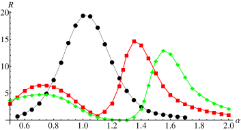
Figure 4: (Color online) Spectral characterization of colored noise: The plot shows the QSNR $R(\tau_{{\rm opt}},\alpha,N)$ as a function of $\alpha$ for different numbers of fluctuators: $N=1$ (black circles), $N=10$ (red squares) and $N=50$ (green rhombuses). Lines are guides for the eyes.

To complete our analysis we also investigate with some more details the dependence of the QFI on the structure of the environment, i.e. on the number of fluctuators describing the environment. In Fig. 5 we show the number of fluctuators $N_{\max}$ maximizing the QFI as a function of $\alpha$. We first notice that there is indeed a dependence, and that $N_{\max}$ may be considerably different for, say, pink or brown noise. As it is apparent from Fig. 5 $N_{\max}$ decreases with increasing $\alpha$ until it reaches the value $N_{\max}=1$ for values of $\alpha$ close to 1. Then it increases with $\alpha$, up to $N_{\max}=540$ for $\alpha=2$.

As a final remark, we also notice that when the number of fluctuators is taken equal to $N_{\max}$, than the optimal interaction time maximizing the QFI is $\tau\simeq\pi/2$ independently on $\alpha$.

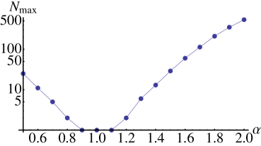
Figure 5: (Color online) Spectral characterization of colored noise: The plots shows the number of fluctuators $N_{\max}$ that maximizes the QFI as a function of the exponent $\alpha$. The line is a guide for the eyes.

IV Conclusions

In this paper we have addressed the estimation of the spectral properties of classical environments using a qubit as a quantum probe. In particular, we have focused attention on the estimation of the switching rate $\gamma$ of random telegraph noise and of the exponent of colored noise with $1/f^{\alpha}$ spectrum. In both cases we have evaluated the quantum Fisher information and found the optimal initial preparation and the optimal interaction time that maximize its value. We have also shown that population measurement on the qubit is optimal, that is the Fisher information coincides with the quantum Fisher information.

For random telegraph noise the (maximized) QFI is inversely proportional to the square of the switching rate, meaning that the quantum signal-to-noise ratio is constant and thus the switching rate may be estimated with uniform precision in its whole range of variation. The corresponding value of the optimal interaction time decreases with increasing $\gamma$ and is located at multiple of $\pi/2$ in the slow RTN regimes, whereas it grow linearly with $\gamma$ in the fast RTN regime.

For colored noise, we studied the estimability of the color of the spectrum, i.e. of the exponent $\alpha$. Our results show that two different cases emerges: if the environment is modeled by a single random fluctuator, then estimation is more precise for pink noise, i.e. for $\alpha=1$. On the other hand, when the environment is instead described as a collection of several fluctuators, the QFI is has two local maxima, whose positions drift towards the boundaries of the interval $[0.5,2]$ as $N$ is increased. The largest quantum signal-to-noise ratio is obtained for brown noise, i.e. for $\alpha\simeq 2$. We also find that for any fixed value of $\alpha$ there is a specific number of fluctuators maximizing the QFI for the interaction time $\tau\simeq\pi/2$, independently on the value of $\alpha$.

Overall, our results show that the features of a complex environment may be reliably determined by monitoring a small quantum probe with more easily controllable degrees of freedom. In particular, our results show that quantum probes permit to reliably estimate the characteristic parameters of classical noise using measurements performed after a fixed optimal interaction time, rather than collecting a series of measurements to estimate the autocorrelation function of the underlying stochastic process.

Appendix A Series representation for $\Lambda(\tau,\alpha)$

Using the expression (9) of the distribution $p_{\alpha}(\gamma)$ Eq. (12) may be rewritten as

$$\Lambda(\tau,\alpha)= N_{\alpha}(\gamma_{1},\gamma_{2})\int^{\gamma_{2}}_{\gamma_{1}}\!\!d\gamma\,e^{-\gamma\tau}\gamma^{-\alpha}$$

$$\times\Big{[}\cosh\delta\tau+\gamma\tau\frac{\sinh\delta\tau}{\delta\tau}\Big{]}$$ (32)

where $\delta=\sqrt{\gamma^{2}-4}$ and the normalization reads as follows

$$N_{\alpha}(\gamma_{1},\gamma_{2})=\left\{\begin{array}[]{ll}\frac{1}{\ln\gamma_{2}-\ln\gamma_{1}}&\alpha=1\\ &\\ (\alpha-1)\left[\frac{(\gamma_{1}\gamma_{2})^{\alpha-1}}{\gamma_{2}^{\alpha-1}-\gamma_{1}^{\alpha-1}}\right]&\alpha\neq 1\end{array}\right.\,.$$ (36)

Using the new variable $y=\gamma\tau$ we may write

$$\Lambda(\tau,\alpha)=N_{\alpha}(\gamma_{1},\gamma_{2})\Big{[}F(\gamma_{2}\tau,\alpha,\tau)-F(\gamma_{1}\tau,\alpha,\tau)\Big{]}\,,$$ (37)

where

$$F(y,\alpha,\tau)=\tau^{\alpha-1}\Big{[}F_{1}(y,\alpha,\tau)+F_{2}(y,\alpha,\tau)\Big{]}\,,$$

and

$$F_{1}(y,\alpha,\tau) =\int\!\!dy\,e^{-y}\,y^{-\alpha}\,\cosh\sqrt{y^{2}-4\tau^{2}}\,,$$ (38)

$$F_{2}(y,\alpha,\tau) =\int\!\!dy\,e^{-y}\,y^{-\alpha+1}\,\frac{\sinh\sqrt{y^{2}-4\tau^{2}}}{\sqrt{y^{2}-4\tau^{2}}}\,.$$ (39)

Upon expanding the hyperbolic functions and using the relation

$$\int\!\!dy\,e^{-y}\,y^{-\alpha}\,(y^{2}-4\tau^{2})^{k}= \sum_{p=0}^{k}\,(-)^{1+k+p}\,(2\tau)^{2(k-p)}$$

$$\times\left(\begin{array}[]{c}k\\ p\end{array}\right)\Gamma(2p+1-\alpha,y)\,,$$ (42)

where $\Gamma(a,x)$ is the (incomplete) Euler Gamma function, the two functions $F_{k}$ may be rewritten as

$$F_{1}(y,\alpha,\tau)= \sum_{k=0}^{\infty}\sum_{p=0}^{k}\,(-)^{1+k+p}\,\frac{\tau^{2(k-p)}}{(2k)!}$$

$$\times\left(\begin{array}[]{c}k\\ p\end{array}\right)\Gamma(2p+1-\alpha,y)\,,$$ (45)

$$F_{2}(y,\alpha,\tau)= \sum_{k=0}^{\infty}\sum_{p=0}^{k}\,(-)^{1+k+p}\,\frac{\tau^{2(k-p)}}{(2k+1)!}$$

$$\times\left(\begin{array}[]{c}k\\ p\end{array}\right)\Gamma(2p+2-\alpha,y)\,.$$ (48)

We now introduce the new index $s=k-p$ and rearrange series as

$$\sum_{k=0}^{\infty}\sum_{p=0}^{k}...=\sum_{p=0}^{\infty}\sum_{k=p}^{\infty}...=\sum_{p=0}^{\infty}\sum_{s=0}^{\infty}...\,,$$

thus arriving at

$$F_{1}(y,\alpha,\tau)= \sum_{p=0}^{\infty}\sum_{s=0}^{\infty}\frac{(-)^{1+s}}{[2(p+s)]!}\left(\begin{array}[]{c}p+s\\ s\end{array}\right)(2\tau)^{s}$$ (51)

$$\times\Gamma(2p+1-\alpha,y)$$

$$= -\sum_{p=0}^{\infty}\frac{1}{(2p)!}\,\Phi_{p+\frac{1}{2}}(-\tau^{2})\,\Gamma(2p+1-\alpha,y)\,,$$ (52)

where $\Phi_{n}(x)$ denotes the confluent hypergeometric function ${}_{0}F_{1}(n,x)$. Analogously, we arrive at

$$F_{2}(y,\alpha,\tau)= -\sum_{p=0}^{\infty}\frac{1}{(2p+1)!}\,\Phi_{p+\frac{3}{2}}(-\tau^{2})\,\Gamma(2p+2-\alpha,y)\,.$$ (53)

Upon substituting Eqs. (52) and (53) in Eq. (37) we obtain a series representation for the quantity $\Lambda(\tau,\alpha)$. As a matter of fact, truncating the series at the first term, i.e. $p=0$ in Eqs. (52) and (53), already provides an excellent approximation for $\alpha\gtrsim 3/2$ and any value of $\tau$. In formula

$$\Lambda(\tau,\alpha)\simeq \frac{1}{2}N_{\alpha}(\gamma_{1},\gamma_{2})\tau^{\alpha-2}\big{[}2\tau\cos 2\tau\,\Gamma(1-\alpha,\gamma_{1}\tau,\gamma_{2}\tau)$$

$$+\sin 2\tau\,\Gamma(2-\alpha,\gamma_{1}\tau,\gamma_{2}\tau)\big{]},$$ (54)

where $\Gamma(a,x,y)=\Gamma(a,x)-\Gamma(a,y)$. On the other hand, for $\alpha\lesssim 3/2$ the number of terms needed for a reliable approximation rapidly grows.

References

- (1) P. Szakowski, M. Trippenbach, and Y. B. Band, Phys. Rev. E 87, 052112 (2013).
- (2) A. I. Nesterov, G. P. Berman, Phys. Rev. A 85, 052125 (2012).
- (3) Y. M. Galperin, B. L. Altshuler, J. Bergli, and D. V. Shantsev, Phys. Rev. Lett. 96, 097009 (2006).
- (4) D. Crow, R. Joynt, arXiv:1309.6383v1.
- (5) J. Helm, W. T. Strunz, S. Rietzler, and L. E. Warflinger, Phys. Rev. A 83, 042103 (2011).
- (6) H. E. Hurst, Trans. Am. Soc. Civil. Eng. 116, 770 (1951).
- (7) D. B. Percival, Metrologia 40, S289 (2003).
- (8) J. Barunik, L. Kristoufek, Physica A 389, 3844 (2010).
- (9) C. M. Kendziorski, J. B. Bassingthwaighte, P. J. Tonellato, Physica A 273, 439 (1999).
- (10) L. A. Salomon, J. C. Fort, J. Stat. Comp. Simul. 83, 542 (2013).
- (11) M. Magdziarz, J. K. Slezak, J. Wojcik, J. Phys. A 46, 325003 (2013).
- (12) J. Bergli, Y. M. Galperin and B. L. Altshuler, New J. Phys. 11 025002 (2009).
- (13) C. Benedetti, F. Buscemi, P. Bordone, M. G. A. Paris, Int. J. Quantum Inf. 10, 1241005 (2012).
- (14) P. Bordone, F. Buscemi, and C. Benedetti, Fluct. Noise Lett. 11, 1242003 (2012).
- (15) M. B. Weissman Rev. Mod. Phys. 60 537 (1998).
- (16) E. Paladino, Y. M. Galperin, G. Falci, B. L. Altshuler, arXiv:1304.7925v1.
- (17) C. Benedetti, F. Buscemi, P. Bordone, M. G. A. Paris, Phys. Rev. A 87, 052328 (2013).
- (18) F. Buscemi, P. Bordone, Phys. Rev. A 87, 042310 (2013).
- (19) C. W. Helstrom, Quantum Detection and Estimation Theory (Academic Press, New York, 1976).
- (20) J. D. Malley, J. Hornstein, Statist. Sci. 8, 433 (1993).
- (21) S. Braunstein, C. Caves, Phys. Rev. Lett. 72, 3439 (1994).
- (22) D. C. Brody, L. P. Hughston, Proc. Roy. Soc. Lond. A 454, 2445 (1998); A 455, 1683 (1999).
- (23) M. G. A. Paris, Int. J. Quant. Inf. 7, 125 (2009).
- (24) B. M. Escher, L. Davidovich, N. Zagury, R. L. de Matos Filho, Phys. Rev. Lett. 109, 190404 (2012); B. M. Escher, R. L. de Matos Filho, and L. Davidovich, Braz. J. Phys. 41, 229 (2011).
- (25) M. Hotta, T. Karasawa, M. Ozawa, Phys. Rev. A 72, 052334 (2005).
- (26) A. Monras, M. G. A. Paris Phys. Rev. Lett. 98, 160401 (2007).
- (27) A. Fujiwara, Phys. Rev. A 63, 042304 (2001); A. Fujiwara, H. Imai, J. Phys. A 36, 8093 (2003).
- (28) Z. Ji, G. Wang, R. Duan, Y. Feng, M. Ying IEEE Trans. Inf. Theory, 54, 5172 (2008).
- (29) V. D’Auria, C. de Lisio A. Porzio, S. Solimeno, and M. G. A. Paris J. Phys. B 39, 1187 (2006).
- (30) G. Brida, I. Degiovanni, A. Florio, M. Genovese, P. Giorda, A. Meda, M. G. A. Paris, A. Shurupov, Phys. Rev. Lett. 104, 100501 (2010).
- (31) G. Brida, I. P. Degiovanni, A. Florio, M. Genovese, P. Giorda, A. Meda, M. G. A. Paris, and A. P. Shurupov, Phys. Rev. A 83, 052301 (2011) .
- (32) R. Blandino, M. G. Genoni, J. Etesse, M. Barbieri, M. G. A. Paris, P. Grangier, and R. Tualle-Brouri, Phys. Rev. Lett. 109, 180402 (2012).
- (33) C. Benedetti, A. P. Shurupov, M. G. A. Paris, G. Brida, and M. Genovese, Phys. Rev. A 87, 052136 (2013).
- (34) A. Monras, F. Illuminati Phys. Rev. A 81, 062326 (2010); Phys. Rev. A 83, 012315 (2011).
- (35) D. Braun, J. Martin, Nat. Comm. 2, 223 (2011); O. Pinel, P. Jian, N. Treps, C. Fabre, and D. Braun Phys. Rev. A 88, 040102(R) (2013)
- (36) A. Monras, preprint ArXiv:1303.3682.
- (37) A. Monras, Phys. Rev. A 73, 033821 (2006).
- (38) M. Kacprowicz, R. Demkowicz-Dobrzanski, W. Wasilewski, K. Banaszek, I. A. Walmsley, Nature Phot. 4, 357 (2010).
- (39) H. Cable, G. A. Durkin, Phys. Rev. Lett. 105, 013603 (2010).
- (40) G. A. Durkin, New J. Phys. 12 023010 (2010).
- (41) M. G. Genoni, S. Olivares, M. G. A. Paris, Phys. Rev. Lett. 106, 153603 (2011); M. G. Genoni, S. Olivares, D. Brivio, S. Cialdi, D. Cipriani, A. Santamato, S. Vezzoli, M. G. A. Paris, Phys. Rev. A 85, 043817 (2012).
- (42) N. Spagnolo, C. Vitelli, V. G. Lucivero, V. Giovannetti, L. Maccone, and F. Sciarrino, Phys. Rev. Lett. 108, 233602 (2012).
- (43) P. Zanardi, M. G. A. Paris, L. Campos-Venuti, Phys. Rev. A 78, 042105 (2008).
- (44) C. Invernizzi, M. Korbmann, L. Campos-Venuti, M. G. A. Paris, Phys. Rev. A 78, 042106 (2008).
- (45) M. Brunelli, S. Olivares, M. G. A. Paris, Phys. Rev. A 84, 032105 (2011); M. Brunelli, S. Olivares, M. Paternostro, M. G. A. Paris, Phys. Rev. A 86, 012125 (2012).
- (46) C. Benedetti, F. Buscemi, P. Bordone, M. G. A. Paris, Int. J. Quant. Inf. 10, 1241005 (2012).
- (47) R Lo Franco, A D’Arrigo, G Falci, G Compagno and E Paladino, Physica Scripta T147, 014019 (2012).
- (48) B. Abel and F. Marquardt, Phys. Rev. B 78, 201302(R) (2008).
- (49) C. Benedetti, M. G. A. Paris and S. Maniscalco, arXiv:1309.5270v2.
- (50) O. E. Barndorff-Nielsen, R. D. Gill, J. Phys. A 33, 4481 (2000).
- (51) A. Luati, Annals of Statistics 32, 1770, (2004).
- (52) X.-M. Lu, X. Wang, C. P. Sun, Phys. Rev. A 82, 042103 (2010).