Renormalization and Scaling in Quantum Walks

Abstract

We show how to extract the scaling behavior of quantum walks using the renormalization group (RG). We introduce the method by efficiently reproducing well-known results on the one-dimensional lattice. As a nontrivial model, we apply this method to the dual Sierpinski gasket and obtain its exact, closed system of RG-recursions. Numerical iteration suggests that under rescaling the system length, $L^{\prime}=2L$, characteristic times rescale as $t^{\prime}=2^{d_{w}}t$ with the exact walk exponent $d_{w}=\log_{2}\sqrt{5}=1.1609\ldots$. Despite the lack of translational invariance, this is very close to the ballistic spreading, $d_{w}=1$, found for regular lattices. However, we argue that an extended interpretation of the traditional RG formalism will be needed to obtain scaling exponents analytically. Direct simulations confirm our RG-prediction for $d_{w}$ and furthermore reveal an immensely rich phenomenology for the spreading of the quantum walk on the gasket. Invariably, quantum interference localizes the walk completely with a site-access probability that declines with a powerlaw from the initial site, in contrast with a classical random walk, which would pass all sites with certainty.

I Introduction

Following Grover’s work,Grover (1997) it was shown that discrete-time quantum walksAharonov et al. (2001); Shenvi et al. (2003); Bach et al. (2004); Ambainis et al. (2005); Portugal (2013) can access any chosen site of a regular lattice in two or more dimensions at least in $O(\sqrt{N\ln N})$ steps. Such a quadratic speed-up over classical $O(N)$ first-passage times is one of the promising aspects of quantum computing, for instance, to search for items in an unsorted list. The fundamental importance of search algorithms to databases can not be overstated, especially for hierarchical networks without translational invariance. We only need to mention Google’s page-rank algorithm, for which a quantum version was recently proposed.Paparo et al. (2013) As fundamental as the random walk is to the description of classical diffusion and transport phenomena in physicsWeiss (1994); Redner (2001) or the mixing times of randomized algorithms in computer sciences,Moore and Mertens (2011) the analogous quantum walk is rapidly rising in importance to describe a range of phenomena. Already, there are a number of experimental realizations of quantum walks, such as in waveguides,Perets et al. (2008); Martin et al. (2011) photonics,Sansoni et al. (2012); Crespi et al. (2013) and optical lattices.Weitenberg et al. (2011) Therefore, classifying the physical behavior of quantum walks, their entanglement, localization, and interference effects in complex environments, is interesting in its own right.

To date, only very few analytical meansPortugal (2013); Carteret et al. (2003) exist to describe the wealth of experimental and numerical observations. Aside from path-integral methods, these are mostly based on using a Fourier decomposition of the walk equation that presupposes a translational or re-labeling symmetry between all sites. Accordingly, the general quantum walk on a simple line is by now relatively well explored,Aharonov et al. (2001); Shenvi et al. (2003); Bach et al. (2004) with a few forays into specific instances of two-dimensional lattices.Mackay et al. (2002); Ambainis et al. (2005); Oliveira et al. (2006) However, insistence on translational invariance leaves us with a limited understanding of the full impact of quantum interference effects, which are the origin of the quadratic speed-up in the spreading on regular lattices. However, the range of studied systems remains too narrow to assess – let alone, predict – how interference causes any particular scaling. In addition, localization effects emerge as soon as lattices possess loopsInui and Konno (2005); Inui et al. (2005); Falkner and Boettcher (2014) or disorder.Shikano and Katsura (2010)

Here, we develop the venerable real-space renomalization group (RG)Wilson (1971); Goldenfeld (1992); Pathria (1996) to discover the long-range behavior of discrete-time quantum walks in more complex geometries. We introduce RG for the simple line, where we show how to reproduce the well-known ballistic spreading exponent, $d_{w}=1$, by extending the traditional fixed point analysis into the complex plane.Boettcher et al. (2013) For quantum walks on the dual Sierpinski gasket (DSG), iterating our exact recursions to $k=21$ generations, corresponding to a gasket with $N\approx 3^{21}\approx 10^{10}$ nodes, shows that time $t$ rescales with base-line length $L$ as $t\sim L^{d_{w}}$ with $d_{w}=1.16096\ldots=\log_{2}\sqrt{5}$, not quite ballistic but spreading faster than a random walk on DSG,Weber et al. (2010) for which $d_{w}^{RW}=\log_{2}5$. However, we find that localization effects diminish the magnitude of the wave function almost everywhere by $\left|\psi\right|\sim L^{-\beta}$ with $\beta=0.424(3)$, such that extensive transport (that can still reach the boundaries for increasing $L$) decays with a power of $L$ that is bounded between $d_{w}$ and $d_{w}+2\beta$, and we have $1<d_{w}<d_{w}+2\beta<d_{w}^{RW}$. We test our predictions with direct simulations on DSG with up to $k=12$ generations.

This paper is organized as follows. In the next section, we introduce a formulation of the walk problem that allows to study classical and quantum walks on comparable footing. In Sec. III, we apply the RG for walks, classical and quantum, on the simple line. In Sec. IV, we study the RG for the dual Sierpinski gasket. In Sec. V, we discuss the unusual aspects of the RG for quantum walks. In Sec. VI, we conclude with a summary of our results and outline future work.

II Formulation of the Walk Problem

The generic master-equation for a discrete-time walk with a coin, whether classical or quantum, is

$$\left|\Psi\left(t+1\right)\right\rangle={\cal U}\left|\Psi\left(t\right)\right\rangle,$$ (1)

where the time-evolution operator (or propagator) is written as

$${\cal U}={\cal S}\left({\cal C}\otimes{\cal I}\right),$$ (2)

containing the “shift” operator ${\cal S}$ and the coin ${\cal C}$. In the $d$-dimensional site-basis $\left|\vec{n}\right\rangle$, we can describe the state of the system in terms of the site amplitudes $\psi_{\vec{n},t}=\left\langle\vec{n}|\Psi\left(t\right)\right\rangle$, simply the probability density to be at that site for a classical walk, but representing in the quantum walk a vector in coin-space with each component holding the amplitude for transitioning out of site $\vec{n}$ along one of its links. Application of the coin ${\cal C}$ entangles these components, with subsequent redistribution of the walk to neighboring sites by the shift operator ${\cal S}$, based on those amplitudes. On the line, the shift operator for a homogeneous nearest-neighbor walk is

$${\cal S}=\sum_{x}\left\{P\otimes\left|x-1\right\rangle\left\langle x\right|+Q\otimes\left|x+1\right\rangle\left\langle x\right|+R\otimes\left|x\right\rangle\left\langle x\right|\right\}$$ (3)

with the shift matrices $P$ and $Q$ for moving left or right, and $R$ for staying in place, for instance,

$$P=\left(\begin{array}[]{cc}1&0\\ 0&0\end{array}\right),\quad Q=\left(\begin{array}[]{cc}0&0\\ 0&1\end{array}\right),\quad R=\left(\begin{array}[]{cc}0&0\\ 0&0\end{array}\right).$$ (4)

From Eq. (2), we get the propagator

$${\cal U}=\sum_{x}\left\{A\otimes\left|x-1\right\rangle\left\langle x\right|+B\otimes\left|x+1\right\rangle\left\langle x\right|+M\otimes\left|x\right\rangle\left\langle x\right|\right\}$$ (5)

with $A=P{\cal C}$, $B=Q{\cal C}$, and $M=R{\cal C}$, and the unitary coin-matrix ${\cal C}$, most generally,Portugal (2013)

$${\cal C}=\left(\begin{array}[]{cc}\sin\eta&e^{i\chi}\,\cos\eta\\ e^{i\vartheta}\,\cos\eta&-e^{i\left(\chi+\vartheta\right)}\,\sin\eta\end{array}\right).$$ (6)

In a quantum walk, the “hopping” operators $A$, $B$, and $M$ are constrained by the requirement of unitary propagation, ${\cal I}={\cal U}^{\dagger}{\cal U},$ which give the conditions in coin-space,

$${\cal I}_{d} = A^{\dagger}A+B^{\dagger}B+M^{\dagger}M,$$

$$0 = A^{\dagger}M+M^{\dagger}B=A^{\dagger}B,$$ (7)

implying that $A+B+M$ is unitary. As ${\cal C}$ is unitary, these conditions equally apply to $P$, $Q$, and $R$. They can not be satisfies by scalars (except for trivial cases).Meyer (1996); Portugal et al. (5166)

The algebra in Eq. (7) requires at least two-dimensional matrices, and matching the dimension $c$ of the coin space and the degree of each site represents a natural and commonly studied choice. For the $d$-dimensional hypercubic lattice, this means $c=2d$, but higher dimensional coinsInui et al. (2005); Falkner and Boettcher (2014) and even coinless alternativesMeyer (1996); Patel et al. (2005); Falk (2013); Ambainis et al. (0172); Portugal et al. (5166) have been studied.

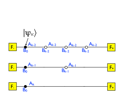
Figure 1: (Color Online) Absorption model for a simple line, indicating the three final recursion steps. Boxes represent absorbing sites, black-marked sites the initial conditions $\left|\psi_{IC}\right\rangle$. Labels $A$ and $B$ indicate the respective hopping parameters for each site.

III Renormalization of the Quantum Walk on a Line

We introduce generating functions,Redner (2001); Boettcher et al. (2008)

$$\tilde{\psi}_{x}\left(z\right)={\textstyle\sum_{t=0}^{\infty}}\psi_{x,t}z^{t},$$ (8)

to eliminate the explicit time-dependence, which allows us to obtain the RG-recursions. The asymptotic behavior for $t\to\infty$ is obtained in the limit of $z\to 1$, which puts more weight on terms with high values of $t$ in Eq. (8). In the inverse-transform of Eq. (8), the limit $z\to 1$ is intimately related to the large-time limit due to the cross-over at $t(1-z)\sim 1$ in $z^{t}=\exp\{t\ln z\}\sim\exp\{-t(1-z)\}$, see Ref. Redner (2001) or any textbook on generating functions.

The master equation (1) with ${\cal U}$ in Eq. (5) then becomes

$$\tilde{\psi}_{x}=zM\tilde{\psi}_{x}+zA\tilde{\psi}_{x-1}+zB\tilde{\psi}_{x+1}+\delta_{x,0}\psi_{IC}.$$ (9)

For simplicity, we merely consider initial conditions (IC) localized at the origin, $\psi_{x,t=0}=\delta_{x,0}\psi_{IC}$. As depicted in Fig. 1, we recursively eliminate $\tilde{\psi}_{x}$ for all sites for which $x$ is an odd number, then set $x\to x/2$ and repeat, step-by-step for $k=0,1,2,\ldots$. Each such step corresponds to a rescaling of the system size by a factor of 2, and after $k$ iterations, $\tilde{\psi}_{x}^{(k)}$ represents the renormalized wave-function describing a domain of size $2^{k}$, and the corresponding renormalized hopping parameters describe the effective transport in and out of that domain.

To wit, starting at $k=0$ with the “raw” hopping coefficients $A_{0}=zA$, $B_{0}=zB$, and $M_{0}=zM$, after each step, the master equation becomes self-similar in form when redefining the renormalized hopping coefficients $A_{k}$, $B_{k}$, $M_{k}$. For example, for consecutive sites near any even site $x$ at step $k$ we have:Boettcher et al. (2013)

$$\tilde{\psi}_{x-1} = M_{k}\tilde{\psi}_{x-1}+A_{k}\tilde{\psi}_{x-2}+B_{k}\tilde{\psi}_{x},$$

$$\tilde{\psi}_{x} = M_{k}\tilde{\psi}_{x}+A_{k}\tilde{\psi}_{x-1}+B_{k}\tilde{\psi}_{x+1}+\delta_{x,0}\psi_{IC},$$ (10)

$$\tilde{\psi}_{x+1} = M_{k}\tilde{\psi}_{x+1}+A_{k}\tilde{\psi}_{x}+B_{k}\tilde{\psi}_{x+2}.$$

Solving for the central site $x$ yields

$$\tilde{\psi}_{x}=M_{k+1}\tilde{\psi}_{x}+A_{k+1}\tilde{\psi}_{x-2}+B_{k+1}\tilde{\psi}_{x+2}+\delta_{x,0}\psi_{IC},$$ (11)

with RG “flow”

$$A_{k+1} = A_{k}\left(I-M_{k}\right)^{-1}A_{k},$$

$$B_{k+1} = B_{k}\left(I-M_{k}\right)^{-1}B_{k},$$ (12)

$$M_{k+1} = M_{k}+A_{k}\left(I-M_{k}\right)^{-1}B_{k}+B_{k}\left(I-M_{k}\right)^{-1}A_{k},$$

where the hopping parameters in general are matrices.

III.0.1 Example: RG for the Classical Random Walk

In the classical analysisRedner (2001); Boettcher et al. (2008) for a random walk with a Bernoulli coin $p$, Eqs. (12) reduce to

$$a_{k+1} =\frac{a_{k}^{2}}{1-m_{k}},$$

$$b_{k+1} =\frac{b_{k}^{2}}{1-m_{k}},$$ (13)

$$m_{k+1} =m_{k}+\frac{2a_{k}b_{k}}{1-m_{k}},$$

with scalar quantities, which initiate at $k=0$ with $a_{0}=zp$, $b_{0}=z\left(1-p\right)$, and $m_{0}=0$. The fixed points (FP) arising from this RG-flow for $k\sim k+1\to\infty$ at $z\to 1$ are $\left(a_{\infty},b_{\infty},m_{\infty}\right)=(0,0,m_{\infty})$, $\left(1-m_{\infty},0,m_{\infty}\right)$, or $\left(0,1-m_{\infty},m_{\infty}\right)$ for any value of $m^{*}$ on the unit interval.

Perturbing the RG-flow in Eqs. (13) via $\{a,b,m\}_{k}\sim\{a,b,m\}_{\infty}+(1-z)\{\alpha,\beta,\mu\}_{k}$ for $z\to 1$ and large $k$, we find the linear system $(\alpha,\beta,\mu)_{k+1}=J\circ(\alpha,\beta,\mu)_{k}$ with the Jacobian

$$J = \left.\frac{\partial\left(a_{k+1},b_{k+1},m_{k+1}\right)}{\partial\left(a_{k},b_{k},m_{k}\right)}\right|_{k\to\infty},$$ (14)

$$= \left(\begin{array}[]{ccc}\frac{2a_{\infty}}{1-m_{\infty}},&0,&\frac{2b_{\infty}}{1-m_{\infty}}\\ 0,&\frac{2b_{\infty}}{1-m_{\infty}},&\frac{2a_{\infty}}{1-m_{\infty}}\\ \frac{a_{\infty}^{2}}{\left(1-m_{\infty}\right)^{2}},&\frac{b_{\infty}^{2}}{\left(1-m_{\infty}\right)^{2}},&1+\frac{2a_{\infty}b_{\infty}}{\left(1-m_{\infty}\right)^{2}}\end{array}\right).$$ (18)

The largest eigenvalue $\lambda_{w}$ of this Jacobian, via $t(1-z)\sim 1$, then describes how time rescales, $t_{k}=\lambda_{w}t_{k-1}$, when doubling system length, $L_{k}=2L_{k-1}$. Assuming a similarity solution for the probability density function of the walk, $\rho\left(x,t\right)\sim f\left(x^{d_{w}}/t\right)$, the scaling Ansatz relating distance and time, $t_{k}\sim L_{k}^{d_{w}}$, thus provides

$$d_{w}=\log_{2}\lambda_{w}.$$ (19)

Inserting the 2nd and 3rd FP in $J$ easily yield the ballistic solutions, $d_{w}=1$, for drifting either to the left or to the right only. In contrast, the indeterminedness of $m_{\infty}$ in the 1st FP is peculiar. In fact, for $z=1$, $a_{k}+b_{k}+m_{k}=1$ for all $k$ and starting from symmetric initial values $a_{0}=b_{0}$, i.e., $p=\frac{1}{2}$, both remain identical and vanish together, $a_{k}\equiv b_{k}\to 0$, and $m_{k}\to m_{\infty}=1$. Since both numerators and denominators in the Jacobian vanish, a correlated solution has to be constructed that “peals off” the leading behavior to glance into the boundary layer. Using $a_{k}\equiv b_{k}\sim a_{k}^{\prime}\epsilon^{k}$ and $m_{k}\sim 1-m_{k}^{\prime}\epsilon^{k}$ assuming large $k$ and $\left|\epsilon\right|<1$, results in

$$a_{k+1}^{\prime}=\frac{a_{k}^{\prime 2}}{\epsilon m_{k}^{\prime}},\qquad m_{k+1}^{\prime}=\frac{1}{\epsilon}m_{k}^{\prime}-\frac{2a_{k}^{\prime 2}}{\epsilon m_{k}^{\prime}}$$ (20)

with a single FP that self-consistently determines $\frac{a_{\infty}^{\prime}}{m_{\infty}^{\prime}}=\epsilon=\frac{1}{2}$. The Jacobian of these recursions, $J^{\prime}=\frac{\partial\left(a_{k+1}^{\prime},m_{k+1}^{\prime}\right)}{\partial\left(a_{k}^{\prime},m_{k}^{\prime}\right)}|_{k\to\infty}$, at its FP gives $\lambda_{w}=4$ as the largest eigenvalue, i.e., $d_{w}=2$ for the diffusive solution. In this formulation, even if we start with vanishing self-term initially, $m_{0}=0$, the self-term ultimately dominates, $m_{k}\to 1$, reflecting the fact that in diffusion the renormalized domain of length $L_{k}\sim 2^{k}$ outgrows the walk such that almost all hops remain within that domain.

We note that the RG projects the salient properties of the walk into three “universality classes:” diffusive and ballistic motion either to the left or right, characterized by an exponent $d_{w}=2$ or 1. Each characterizes a fixed point of the dynamics, reached either for $p=\frac{1}{2}$ or $p\not=\frac{1}{2}$.

III.0.2 RG for the Quantum Walk on a Line

For the quantum walk, we set

$$A_{k}=P_{k}{\cal C},\qquad B_{k}=Q_{k}{\cal C},\qquad M_{k}=R_{k}{\cal C},$$ (21)

where initially $P_{0}=zP$, $Q_{0}=zQ$, and $R_{0}=zR$ from Eq. (4). To gain an intuition, we evolve the RG-flow (12) for a few iterations from these raw values. Each iteration consists of assembling the hopping parameters at level $k$ according to Eq. (21), the actual RG-step of applying Eqs. (12), and then of inverting Eq. (21) with ${\cal C}^{-1}$ to arrive at $P_{k+1}$, $Q_{k+1}$, and $R_{k+1}$. Already after two steps, a recurring pattern emerges that suggests the parametrization

$$P_{k}=\left(\begin{array}[]{cc}a_{k}&0\\ 0&0\end{array}\right),\enskip Q_{k}=\left(\begin{array}[]{cc}0&0\\ 0&-a_{k}\end{array}\right),\enskip R_{k}=\left(\begin{array}[]{cc}0&m_{k}\\ m_{k}&0\end{array}\right).$$ (22)

Indeed, for $a_{k}$ and $m_{k}$, the RG-flow (12) closes after each iteration with

$$a_{k+1} = \frac{a_{k}^{2}\sin\eta}{1-2m_{k}\cos\eta+m_{k}^{2}},$$

$$m_{k+1} = m_{k}+\frac{\left(m_{k}-\cos\eta\right)a_{k}^{2}}{1-2m_{k}\cos\eta+m_{k}^{2}}$$ (23)

for $0<\eta<\pi/2$ (setting $\chi=\vartheta=0$). These recursions have a single fixed point at $\left(a_{\infty},m_{\infty}\right)=\left(\sin\eta,\cos\eta\right)$, yet, its Jacobian at $k\to\infty$ is $\eta$-independent and has a degenerate eigenvalue $\lambda_{w}=2$, suggesting $d_{w}=\log_{2}\lambda=1$. This reflects the well-known universality of the large-scale dynamics of the quantum walk on the line with respect to the chosen coin.Bach et al. (2004)

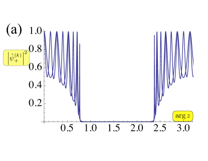
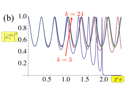
Figure 2: (Color Online) Plot of $\left|\tilde{\psi}_{+}^{\left(k\right)}\left(z\right)\right|$ at $\eta=\pi/4$ and generic initial conditions $\psi_{IC}=\left(0,1\right)$ (a) for $\arg z$ after $k=2,3$ iterations and (b) for the rescaled variable $2^{k}\theta$, $z=-e^{i\theta}$, to collapse all data up to $k=24$ for $\theta\to 0$. As (a) shows, the integrand is periodic with period $\pi$ and has significant support only for $|\theta|<\eta$ and $\pi-|\theta|<\eta$.

As we will show in Sec. V, though, this picture may be incomplete, a lucky accident due to the fact that the “fractal” exponent, $d_{f}=\log_{2}\lambda_{f}=1$, and the walk exponent $d_{w}$ coincide. To exemplify this aspect here, let us consider the probability $F_{a}$ of ever being absorbed at a site $x=a$ as a simple and generic observable.Ambainis et al. (2001); Bach et al. (2004) From Eq. (8), for a random walk with $\rho\left(x,t\right)=\psi_{x,t}$, it is simply $F_{a}=\sum_{t}\psi_{a,t}=\lim_{z\to 1}\tilde{\psi}_{a}\left(z\right)$. For a quantum walk, it is instead $\rho\left(x,t\right)=\left|\psi_{x,t}\right|^{2}$, and hence,

$$F_{a}=\sum_{t=0}^{\infty}\left|\psi_{a,t}\right|^{2}=\oint\frac{dz}{2\pi iz}\,\left|\tilde{\psi}_{a}\left(z\right)\right|^{2}=\int_{-\pi}^{\pi}\frac{d\theta}{2\pi}\,\left|\tilde{\psi}_{a}\left(\theta\right)\right|^{2},$$ (24)

where we choose

$$z=-e^{i\theta}\qquad\left(-\pi<\theta\leq\pi\right),$$ (25)

i.e., $z\to-1$ for $\theta\to 0$ as reference point (see below). While the random walk merely entails a local analysis for real $z\to 1$,Redner (2001) the unitarity of quantum walks generally demands an analysis along the entire unit circle in the complex-$z$ plane. Let us put the quantum walk on the line between two absorbing walls, $F_{\pm}$, as shown in Fig. 1, with $F_{-}^{(k)}$ at $x_{-}=-1$ right next to the starting site $x=0$, from which the wall $F_{+}^{(k)}$ at site $x_{+}=2^{k}$ recedes further away with every iteration of the flow equations. In Fig. 2(a), we plot the integrand $\left|\tilde{\psi}_{+}^{(k)}\left(z\right)\right|$ for $\arg z=\pi-\theta$, on the unit circle. Some algebra shows that $\tilde{\psi}_{+}^{(k)}\left(z\right)\propto a_{k}$, which depends on $z$ through $a_{0}$. The asymptotic behavior of $a_{k}$ in Eq. (23) for large $k$ at fixed $\theta$ falls into one of four different cases: (i) at $\theta=0$ and $\theta=\pi$, the stationary behavior for the aforementioned fixed point is obtained; (ii) for $0<\left|\theta\right|<\eta$ and $0<\pi-\left|\theta\right|<\eta$, $a_{k}$ varies chaotically with $k$; (iii) for $\left|\theta\right|=\eta$ and $\left|\theta\right|=\pi-\eta$ local analysis recovers classical diffusive scaling; and (iv) for $\eta<\left|\theta\right|<\pi-\eta$, $a_{k}$ vanishes exponentially with $N=2^{k}$. We argue that only the chaotic regimes, $\left|\theta\right|<\eta$ and $\pi-\left|\theta\right|<\eta$, with the stationary point at their center contributes to extensive quantum transport. To wit, it can be shown that for $\eta\to 0$ the “velocity” of the ballistically spreading quantum walk decreases to zero and it eventually becomes localized for $\eta=0$, exactly when both chaotic regimes shrink to zero, while the stationary point remains inside.

Clearly, quantum transport here is determined by properties of the entire wave-function, $\tilde{\psi}_{x}\left(z\right)$, not just the limit $z\to z_{0}$ near some fixed point $z_{0}$. We will analyze this situation in more detail in Sec. V.

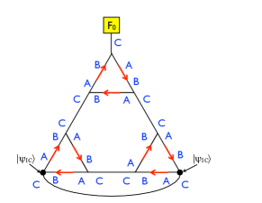
Figure 3: (Color Online) Absorption model for the dual Sierpinski gasket at generation $k=1$. Boxes represent absorbing site, black-marked sites harbor the initial conditions $\left|\psi_{IC}\right\rangle$. Labels $A,B,C$ indicate the respective hopping parameters for leaving each site. Note that for increasing generation $k$, the minimal separation between initiating sites and the sole absorbing site will increase as $\sim 2^{k}$.

IV Renormalization of the Quantum Walk on the Dual Sierpinski Gasket

The DSG is a degree-3 lattice, see Fig. 3, and unitarity requires at least a $c=3$-dimensional coin. As the most general such coin has six real parameters, we focuses here only on the real and symmetric Grover coin,

$${\cal C}=\frac{1}{3}\left(\begin{array}[]{ccc}-1&2&2\\ 2&-1&2\\ 2&2&-1\end{array}\right),$$ (26)

and defer generalizations to future discussions. Note that DSG has several advantages over the more familiar Sierpinski gasket (of which it is dual). DSG is of regular degree 3, while Sierpinski itself is a regular degree-4 lattice. However, it is not merely the higher degree that provides difficulties for quantum walks on the original Sierpinski gasket. The internal coin degrees of freedom provide a labeling problem that severely complicates its consideration, already in evidence in Ref. Lara et al., 2013. Interestingly, none of these problems exist for the classical random walk, and the Sierpinski gasket (or its dual) serves as a popular example of a simple demonstration of the RG, as its hierarchical structure and high degree of symmetry affects an RG-flow in a single real hopping parameter. For the quantum walk, we will find instead five coupled complex recursions with a large number of terms.

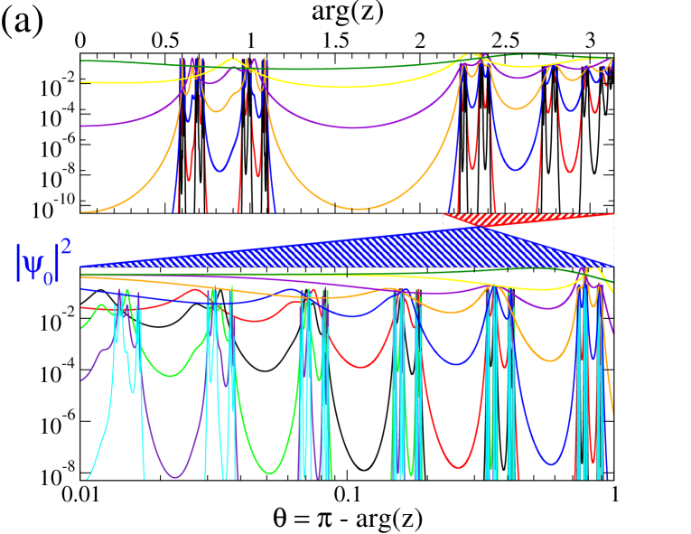
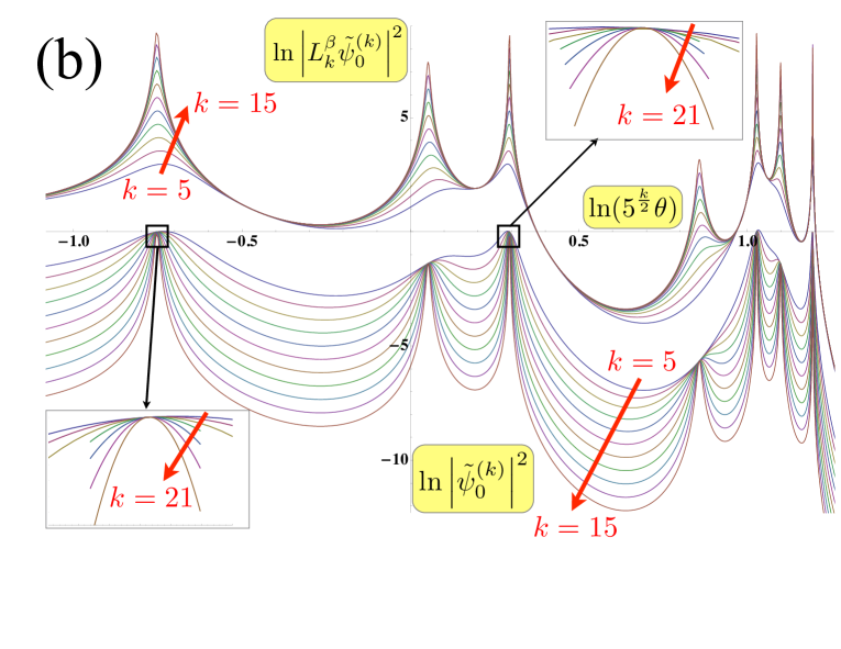
Figure 4: (Color Online) (a) Log-plot of the integrand $\left|\tilde{\psi}_{0}^{\left(k\right)}\left(z\right)\right|$ in Eq. (24) for $0\leq\arg z\leq\pi$ for $k=1,\ldots 6$. Decaying almost everywhere, the integrand has most support near the fixed point, $\arg z\to\pi$. A logarithmic scale with $\theta=\pi-\arg z\to 0$ reveals a self-similar sequence of periodic structures. (b) Scaling collapse of $\left|L_{k}^{\beta}\tilde{\psi}_{0}^{\left(k\right)}\left(z\right)\right|$ with $L_{k}=2^{k}$ for $\ln\left(\lambda_{w}^{k}\theta\right)$ at $k=5,\ldots,15$ using $\lambda_{w}=\sqrt{5}$. At $\beta=0$, all data lines up, in particular, all peaks remain constant (=1 up to $k=21$, see insets) but narrow. At $\beta=0.424(3),$ all data in the fast-decaying intervals collapse but the peaks now diverge.

IV.1 Renormalization of the Dual Sierpinski Gasket

Fig. 3 shows the elementary graph-let of nine sites that is used to construct the dual Sierpinski gasket (DSG). It also represents the basic unit from which we can extract the flow equations by tracing out the wave functions $\tilde{\psi}_{4},\ldots,\tilde{\psi}_{9}$ on the six inner sites to leave only the three corner sites $\tilde{\psi}_{1},\ldots,\tilde{\psi}_{3}$ and the renormalized hopping coefficients between them. Note the systematic labeling for the three out-direction of each site that determines, in effect, which shift operator applies to that direction. The master equations relating those nine sites are:

$$\tilde{\psi}_{1} = M_{k}\tilde{\psi}_{1}+C_{k}\tilde{\psi}_{\bar{1}}+A_{k}\tilde{\psi}_{4}+B_{k}\tilde{\psi}_{5},$$

$$\tilde{\psi}_{2} = M_{k}\tilde{\psi}_{2}+C_{k}\tilde{\psi}_{\bar{2}}+A_{k}\tilde{\psi}_{6}+B_{k}\tilde{\psi}_{7},$$

$$\tilde{\psi}_{3} = M_{k}\tilde{\psi}_{3}+C_{k}\tilde{\psi}_{\bar{3}}+A_{k}\tilde{\psi}_{8}+B_{k}\tilde{\psi}_{9},$$

$$\tilde{\psi}_{4} = M_{k}\tilde{\psi}_{4}+C_{k}\tilde{\psi}_{9}+A_{k}\tilde{\psi}_{5}+B_{k}\tilde{\psi}_{1},$$

$$\tilde{\psi}_{5} = M_{k}\tilde{\psi}_{5}+C_{k}\tilde{\psi}_{6}+A_{k}\tilde{\psi}_{1}+B_{k}\tilde{\psi}_{4},$$ (27)

$$\tilde{\psi}_{6} = M_{k}\tilde{\psi}_{6}+C_{k}\tilde{\psi}_{5}+A_{k}\tilde{\psi}_{7}+B_{k}\tilde{\psi}_{2},$$

$$\tilde{\psi}_{7} = M_{k}\tilde{\psi}_{7}+C_{k}\tilde{\psi}_{8}+A_{k}\tilde{\psi}_{2}+B_{k}\tilde{\psi}_{6},$$

$$\tilde{\psi}_{8} = M_{k}\tilde{\psi}_{8}+C_{k}\tilde{\psi}_{7}+A_{k}\tilde{\psi}_{9}+B_{k}\tilde{\psi}_{3},$$

$$\tilde{\psi}_{9} = M_{k}\tilde{\psi}_{9}+C_{k}\tilde{\psi}_{4}+A_{k}\tilde{\psi}_{3}+B_{k}\tilde{\psi}_{8}.$$

Here, $\tilde{\psi}_{\bar{1}},\ldots,\tilde{\psi}_{\bar{3}}$ refer to the corner sites of the respective neighboring graph-lets, which themselves also do not get renormalized.

It drastically reduces the algebraic effort to trace out $\tilde{\psi}_{4},\ldots,\tilde{\psi}_{9}$ in a symmetrical way. When eliminated, each of those amplitudes must be a function of the remaining three, $\tilde{\psi}_{1},\ldots,\tilde{\psi}_{3}$, in a cyclically permuted manner. Thus, we start with the Ansatz

$$\tilde{\psi}_{4} = a\tilde{\psi}_{1}+b\tilde{\psi}_{2}+c\tilde{\psi}_{3},$$

$$\tilde{\psi}_{5} = d\tilde{\psi}_{1}+e\tilde{\psi}_{2}+f\tilde{\psi}_{3},$$ (28)

and similarly for the inner sites at there other two corners, $\left(\tilde{\psi}_{6},\tilde{\psi}_{7}\right)$ and $\left(\tilde{\psi}_{8},\tilde{\psi}_{9}\right)$, by appropriately permuting the indices on $\tilde{\psi}_{1},\ldots,\tilde{\psi}_{3}$. Inserting these prospective solutions into the right-hand side of the last six relations in Eqs. (27) and comparing coefficients with Eqs. (28) provides self-consistency relations for the matrices $a,\ldots,f$. This step eliminates $\tilde{\psi}_{4},\ldots,\tilde{\psi}_{9}$ by transforming the problem into one of expressing the matrices $a,\ldots,f$ in terms of $A_{k},B_{k},C_{k},$ and $M_{k}$, or with simpler notation: $\bar{A}=\left(I-M_{k}\right)^{-1}A_{k}$, $\bar{B}=\left(I-M_{k}\right)^{-1}B_{k}$, and $\bar{C}=\left(I-M_{k}\right)^{-1}C_{k}$. Most importantly, this Ansatz has disentangled the original six equations into two equivalent, closed sets of three relations that can be solved independently: Since comparing coefficients provides a bipartite set of relations initially,

$$\begin{array}[]{rclcrcl}a&=&\bar{A}d+\bar{C}e+\bar{B},&&d&=&\bar{B}a+\bar{C}c+\bar{A},\\ b&=&\bar{A}e+\bar{C}f,&&e&=&\bar{B}b+\bar{C}a,\\ c&=&\bar{A}f+\bar{C}d,&&f&=&\bar{B}c+\bar{C}b,\end{array}$$ (29)

(noting that these are non-commuting matrices), we write

$$a = \bar{A}\bar{B}a+\bar{A}\bar{C}c+\bar{A}^{2}+\bar{C}\bar{B}b+\bar{C}^{2}a+\bar{B},$$

$$b = \bar{A}\bar{B}b+\bar{A}\bar{C}a+\bar{C}\bar{B}c+\bar{C}^{2}b,$$ (30)

$$c = \bar{A}\bar{B}c+\bar{A}\bar{C}b+\bar{C}\bar{B}a+\bar{C}^{2}c+\bar{C}\bar{A},$$

and an corresponding set for $d,e,f$ by identifying $a\Leftrightarrow d$, $b\Leftrightarrow f$, $c\Leftrightarrow e$, and $\bar{A}\Leftrightarrow\bar{B}$, while $\bar{C}$ remains in place. To minimize the number of matrix-multiplications, it is now convenient to abbreviate

$$V = \left(I-\bar{A}\bar{B}-\bar{C}^{2}\right)^{-1},$$

$${\cal A} = V\bar{A}\bar{C},$$

$${\cal B} = V\bar{C}\bar{B},$$

$$W = \left(I-{\cal B}{\cal A}\right)^{-1},$$ (31)

$$X = {\cal A}^{2}+{\cal B},$$

$$Y = W\left({\cal A}+{\cal B}^{2}\right),$$

$$Z = WV\left(A^{2}+B\right).$$

With those, we find

$$c = \left[I-{\cal A}{\cal B}-XY\right]^{-1}\left(V\bar{C}\bar{A}+XZ\right),$$

$$a = Yc+Z,$$ (32)

$$b = {\cal A}a+{\cal B}c,$$

and the complementing set for $d,e,$ and $f$. Finally, inserting $\tilde{\psi}_{4},\tilde{\psi}_{5}$ from Eqs. (28) into the relation for $\tilde{\psi}_{1}$ (or, respectively, inserting $\tilde{\psi}_{6},\tilde{\psi}_{7}$ into the relation for $\tilde{\psi}_{2}$, or $\tilde{\psi}_{8},\tilde{\psi}_{9}$ for $\tilde{\psi}_{3}$) yields the renormalization-flow

$$M_{k+1} = M_{k}+A_{k}a+B_{k}d,$$

$$A_{k+1} = A_{k}c+B_{k}f,$$

$$B_{k+1} = A_{k}b+B_{k}e,$$ (33)

$$C_{k+1} = C_{k}.$$

(Note that $C_{k}$ does not renormalize.) While tedious to derive, these equations are exact and easily implemented on a computer algebra system.

IV.2 Parametrizing the RG-Flow for the Dual Sierpinski Gasket

Similar to Sec. III.0.2, we define shift matrices

$$P=\left[\begin{array}[]{ccc}1&0&0\\ 0&0&0\\ 0&0&0\end{array}\right],\quad Q=\left[\begin{array}[]{ccc}0&0&0\\ 0&1&0\\ 0&0&0\end{array}\right],\quad R=0.$$ (34)

Since $C_{k}=C_{0}$, it will require no parametrization. We initiate the recursions at $k=0$ with $A_{0}=zPC$, $B_{0}=zQ{\cal C}$, and $M_{0}=zR{\cal C}=0$. After a single iteration, a recursive pattern emerges that suggests a 5-parameter Ansatz:

$$P_{k} = \left(\begin{array}[]{ccc}a_{k}^{(1)}&a_{k}^{(2)}&0\\ a_{k}^{(2)}&a_{k}^{(3)}&0\\ 0&0&0\end{array}\right),\quad Q_{k}=\left(\begin{array}[]{ccc}a_{k}^{(3)}&a_{k}^{(2)}&0\\ a_{k}^{(2)}&a_{k}^{(1)}&0\\ 0&0&0\end{array}\right),$$ (41)

$$R_{k} = \frac{1}{2}\left(\begin{array}[]{ccc}m_{k}^{(1)}-m_{k}^{(2)}&m_{k}^{(1)}+m_{k}^{(2)}&0\\ m_{k}^{(1)}+m_{k}^{(2)}&m_{k}^{(1)}-m_{k}^{(2)}&0\\ 0&0&0\end{array}\right),$$ (45)

Iteration provides of closed set of five complex recursions, $\left\{a_{k+1}^{(1,2,3)},m_{k+1}^{(1,2)}\right\}={\cal R}\left(\left\{a_{k}^{(1,2,3)},m_{k}^{(1,2)}\right\};z\right)$, each a ratio of polynomials similar to Eqs. (23) but with dozens of terms and an explicit dependence on $z$ due to $C_{0}$. Again, the algebra is easily handled on the computer, however, these recursions prove numerically unstable, and numerical precision is quickly lost near points of interest, such as $z=-1$.

IV.3 Asymptotic properties of the RG-flow

As a specific observable to study, we again focus on the probability to ever get absorbed at a wall, as shown in Fig. 3. With increasing length $L$, the sole absorbing site at one corner of DSG recedes from the starting point of the quantum walk (IC), chosen at the opposite corners. Thus, the total absorption $F_{0}^{(k)}$ is a measure of quantum transport across the system. Fig. 4(a) shows the integrand $\left|\tilde{\psi}_{0}^{\left(k\right)}\left(z\right)\right|^{2}$ of $F_{0}$ in Eq. (24) for $0\leq\arg z\leq\pi$ (all observables are symmetric around the real-$z$ axis). We derive the expression for $\tilde{\psi}_{0}$ in Eq. (53) in the Appendix. Compared to Fig. 2(a) for the line, remarkably complex patterns emerge for a quantum walk on DSG:

1. There is an isolated stationary point at $\arg z=\pi$, i.e., $\theta=0$, see Eq. (25), where $a_{k}^{(1,2,3)}=-m_{k}^{(1)}=-\frac{1}{3}$ and $m_{k}^{(2)}=1$ for all $k\geq 2$.

2. A sequence of sparse, rugged peaks that slowly decay seem to accumulate for $\theta\to 0$ with increasing $k$.

3. Everywhere else the function decays rapidly for increasing $k$, where $a_{k}^{(1)}\sim a_{k}^{(2)}\sim a_{k}^{(3)}\to 0$ and $\left|m_{k}^{(1,2)}\right|\to 1$. There is no finite oscillatory domain to signal extensive quantum transport. Instead, since $\tilde{\psi}_{0}^{\left(k\right)}\sim a_{k}^{(1,2,3)}$, it is easy to show from the five recursions that for any fixed value of $\theta\not=0$, $\left|\tilde{\psi}_{0}^{\left(k\right)}\left(z\right)\right|\to 0$ for $k\to\infty$, suggesting that for large systems quantum transport ceases such that the absorption approaches zero.

Unlike for translation-invariant lattices, where some fraction of quantum walks might localize, on DSG the entire walk eventually gets trapped. However, unlike the sharp localization on lattices,Inui et al. (2005); Falkner and Boettcher (2014) the entrapped portion of the wave-function has broad tails here. Only at $\theta=0$ do we find a fixed point. Its Jacobian has a largest eigenvalue of $\lambda_{f}=3$, which coincides with the fractal exponent of DSG, $d_{f}=\log_{2}3$. Yet, the data collapse in Fig. 4(b) demonstrates that the limit $\theta\to 0$ is singular: all data aligns and collapses according to Eq. (46) but with an eigenvalue smaller than the Jacobian. This collapse occurs in a regime such that $\lambda_{w}^{k}\theta\sim 1$, while the fixed point at $\ln\theta\to-\infty$ seems infinitely far away and irrelevant. We will discuss this point in more detail in Sec. V.

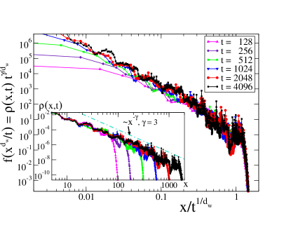
Figure 5: (Color Online) Simulations of quantum walks on DSG for the collapse $f\left(x^{d_{w}}/t\right)\sim\rho\left(x,t\right)t^{\gamma/d_{w}}$ with $d_{w}=\log_{2}\sqrt{5}$ for the probability density function $\rho\left(x,t\right)=\left|\psi_{x,t}\right|^{2}$ (see inset) for finding the walker at any site $x$ hops away from the initial sites at times $t=2^{l}$, $l=7,\ldots,12$, on a DSG of size $N\sim 3^{12}$, before the absorbing wall is reached. To fit not only the cut-off but also the bulk distribution, we estimate a power-law decay with exponent $\gamma\approx 3$ for $\rho$ as a function of $x$, see inset.

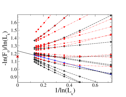
Figure 6: (Color Online) Extrapolation for the scaling exponent in the decay of the simulated absorption $F_{0}$ with system length $L_{k}=2^{k}$, $k\leq 12$, based on a power-law, for many different symmetric ($+$) and asymmetric ($\bullet$) initial conditions (IC). All data appears to extrapolate to the same intercept ($L_{k}\to\infty$) at about $1.23(1)$, with the most linear fit (extended line) provided by the symmetric $\psi_{IC}\propto\left(1,2,1\right)$. This exponent is closely bounded below by $d_{w}=\log_{2}\sqrt{5}$ ($\times$).

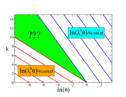
Figure 7: (Color Online) Depiction of the characteristic trajectories along which the RG-flow remains invariant, where $\theta=\arg(z-z_{0})$ is a measure of the angular distance from the fixed point at $z_{0}$ in the complex unit circle. In this picture, the fixed point is off to the left at $\ln\theta=-\infty$, where the data collapses by way of the fractal exponent $d_{f}=\log_{2}\lambda_{f}$ (red trajectories), resulting from the largest Jacobian eigenvalue, $\lambda_{f}$. On the right, where $\lambda_{w}^{k}\theta\gtrsim 1$ (blue trajectories), a far more subtle collapse as that shown in Fig. 4 results. Note that those trajectories can not ever reach the fixed point, since $\lambda_{w}<\lambda_{f}$, and will require some intermediate scaling Ansatz (except for the quantum walk on a line, where $\lambda_{f}=\lambda_{w}$). The green-shaded area between those different characteristics marks an unknown cross-over region.

The exponents $\lambda_{w}$ and $\beta$ from Eq. (46) can be determined recursively with high accuracy from the collapse with computational cost linear in $k$ (i.e., logarithmic in system size). As shown at the bottom of Fig. 4(b) and especially the insets, lining-up the data for $\left|\tilde{\psi}_{0}^{\left(k\right)}\left(z\right)\right|$, $k=5,\ldots,21$, without resizing ($\beta=0$) yields $\lambda_{w}=2.23607(2)$, which we identify as $\lambda_{w}=\sqrt{5}$, such that $d_{w}=\log_{2}\lambda_{w}=\log_{2}\sqrt{5}$. (The only limitation in the ability to determine the value of $\lambda_{w}$ to arbitrary accuracy numerically is set by the chaotic nature of the RG-recursions; initiating $z$ near $\theta\to 0$ with 1500 digits accuracy, none remains after only $k=25$ iterations.)

To demonstrate the relevance of this eigenvalue $\lambda_{w}$ for the asymptotic spreading of the quantum walk, we have conducted large-scale numerical simulations directly of the master equation, see Fig. 5. This value of $d_{w}=\log_{2}\sqrt{5}$ provides data collapse for $\rho\left(x,t\right)\sim f\left(x^{d_{w}}/t\right)/t^{\gamma/d_{w}}$ with $\gamma\approx 3$ from fitting $\rho\left(x,t\right)\sim x^{-\gamma}$, see inset of Fig. 5. (The origin of this power-law decay, in contrast to a Gaussian kernel for diffusion, is of yet unknown.) In particular, the inset shows that the cut-off in $\rho\left(x,t\right)$ scales perfectly as $x_{co}\sim t^{1/d_{w}}$, leading to the collapse in the main panel.

Yet, this shift in $\theta$ alone results in a set of functions that uniformly decay with increasing $k$ everywhere but in isolated points, see down-arrows in Fig. 4(b). Using $\beta=0.424(3)$ in Eq. (46) collapses the data everywhere except for isolated peaks that now grow with $k$, see up-arrows in Fig. 4(b). The absorption integral from Eq. (24) that receives most of its support near $\left|\theta\right|<\epsilon\ll 1$ yields $F_{0}^{(k)}\sim F_{0}^{(k-1)}/\left(\lambda_{w}2^{2\beta}\right)$, using Eq. (46), with solution $F_{0}^{(k)}\sim L_{k}^{-(d_{w}+2\beta)}$, $L_{k}\sim 2^{k}$, as a lower bound on the adsorption. Thus, the true $F_{0}^{(k)}$ vanishes with length $L$ as a power law with exponent at least as large as $d_{w}$ ($\beta=0$) but not larger than $d_{w}+2\beta\approx 2.01(1)$. Simulations of quantum walks on DSG up to $k=12$ generations shown in Fig. 6 suggest a unique exponent $\approx 1.23(1)$ that is only minutely above $d_{w}$, independent of the IC.

V How RG-Fixed Points Fail to Determine Asymptotic Properties

As Sec. IV.1 has shown, extracting the scaling $\rho\left(x,t\right)\sim f\left(x^{d_{w}}/t\right)$ from the fixed point proves insufficient for the quantum walk on DSG. While the fixed point of the RG for the quantum walk on the line naively appears to reproduce the known scaling properties, the discussion shows that this is likely a coincidence for this rather simple scenario. The examples of the line in Sec. III and of DSG in Sec. IV shows, the fixed point found in both cases appears to coincide with the fractal exponent, $d_{f}=\log_{2}\lambda_{f}$, that refers to structural properties of the lattice, rather then to the dynamics of the walk itself.

Since most dynamic observables require an extended examination in the complex-$z$ plane, the example of the Sierpinski gasket suggest that the same holds true for the RG-flow. As the data collapse in Fig. 4 demonstrates, the way to extract the eigenvalue $\lambda_{w}$ (and, hence, $d_{w}$) that is consistent with the RG on fractals (such as DSG below) results from the scaling

$$\tilde{\psi}_{a}^{(k)}\left(\theta\right)\sim 2^{-\beta}\tilde{\psi}_{a}^{(k-1)}\left(\lambda_{w}\theta\right)$$ (46)

at large $k$ near a fixed point for $\theta\to 0$, such that $\lambda_{w}^{k}\theta\gtrsim 1$. Rescaling $\theta$ corresponds to $z\to z^{1/\lambda_{w}}$ for $k\to k+1$, and hence, from Eq. (8) we see that it amounts to a rescaling of time $t$ with $\lambda_{w}$ when $L$ doubles, such that $d_{w}=\log_{2}\lambda_{w}$. The scenario posed by Eq. (46) is depicted in Fig. 7, which suggests that the RG-flow will have to be solved asymptotically in an intermediate scaling regime, as it can never reach the fixed point for $\lambda_{w}<\lambda_{f}$. While this has not be achieved yet, the simplicity of the exponent suggests that such an exact analysis should be possible. It suggests that the RG for quantum walks requires an entirely new approach, beyond the usual fixed point analysis.

The fixed-point analysis happened to be successful for the 1d-line because there fractal and walk exponents coincide, $d_{w}=d_{f}=d=1$ (and $\beta=0$ here), as demonstrated by the data-collapse in Fig. 2(b). As the limit $\theta\to 0$ for the simple line is not singular, it is not surprising that scaling collapse and traditional RG analysis near the fixed point provide identical results.

VI Conclusions

In conclusion, we have devised a method to determine the asymptotic behavior of discrete-time quantum walks on the dual Sierpinski gasket using RG. Fractal graphs, as well as random networks, lack the translational symmetry that is essential to study quantum walks on lattices. The present treatment can be applied to renormalizable structures,Redner (2001) ultimately to generate analytical results for important physical quantities such as the spreading rate of the probability distributions. However, compared to random walks, quantum walks require extending RG into the complex plane, which we have explored in some detail. We confirmed that quantum walks are more intricate than random walks, and we analyzed the effects of geometry on quantum interference. Direct numerical simulations support our conclusions.

The RG analysis for quantum walks appears to be more complicated than for classical random walks, a likely result of unitarity, which precludes the typical contractive mapping that makes RG of classical, stochastic processes easy. Yet, our results suggest that such quantum systems will ultimately find just as exact a description as those for classical systems. In turn, much more will be gained, as these quantum processes exhibit a far richer phenomenology compared to the rather structureless diffusion process.

Finally, we note that the potential scope of RG is much broaderGoldenfeld (1992) than merely as a toll to calculate exponents for some specific fractals, where it happens to be exact. Once the present technical issues have been resolved, it should be possible to use the RG, exactly or approximately, to classify the asymptotic properties of quantum walks, and hopefully other quantum algorithms, into universality classes. Such a classification ultimately should serve as the basis for understanding, and hence, control of the observed behaviors.

Appendix

VI.1 Absorption on the Line

We consider the case of two absorbing walls on both ends of the simple line with the initial conditions (IC) located on a single site right next to the left wall, as shown in Fig. 1a. It is convenient to identify the IC-site as the origin ($i=0$), i.e., the left-absorbing site is $\tilde{\psi}_{-}$, and the right wall is located on site $i=2^{k}$ with $\tilde{\psi}_{+}$. Since nothing escapes out of the absorbing sites, we have the master equations:

$$\tilde{\psi}_{-} = B_{0}\tilde{\psi}_{0},$$

$$\tilde{\psi}_{0} = N_{0}\tilde{\psi}_{0}+B_{0}\tilde{\psi}_{1}+\psi_{IC},$$ (47)

$$\tilde{\psi}_{x} = M_{0}\tilde{\psi}_{x}+A_{0}\tilde{\psi}_{x-1}+B_{0}\tilde{\psi}_{x+1},\quad\left(1\leq i\leq 2^{k}-2\right),$$

$$\tilde{\psi}_{2^{k}-1} = M_{0}\tilde{\psi}_{2^{k}-1}+A_{0}\tilde{\psi}_{2^{k}-2},$$

$$\tilde{\psi}_{+} = A_{0}\tilde{\psi}_{2^{k}-1},$$

This setup has been chosen exactly such that all quantities renormalize according to the flow in (12), avoiding some of the special considerations typically required near boundaries. The only exception refers to the self-term at $\tilde{\psi}_{0}$: Although initially $N_{0}=M_{0}=0$, its recursion is $N_{k+1}=N_{k}+B_{k}\left(I-M_{k}\right)^{-1}A_{k}$ instead. (This geometry resembles exactly the setup of Ref. Ambainis et al., 2001, with which we can now compare.)

In each recursion-step, every second intervening site still present is eliminated, see the sequence in Fig. 1a. As the last setting suggests, we are left with three relations,

$$\tilde{\psi}_{-} = B_{0}\tilde{\psi}_{0},$$

$$\tilde{\psi}_{0} = N_{k}\tilde{\psi}_{0}+\psi_{IC},$$ (48)

$$\tilde{\psi}_{+} = A_{k}\tilde{\psi}_{0}.$$

We now simply eliminate $\tilde{\psi}_{0}$ to get

$$\tilde{\psi}_{-}^{(k)} = B_{0}\left(1-N_{k}\right)^{-1}\psi_{IC},$$

$$\tilde{\psi}_{+}^{(k)} = A_{k}\left(1-N_{k}\right)^{-1}\psi_{IC}.$$ (49)

VI.2 Absorption on the Dual Sierpinski Gasket

Using the recursions developed in Eqs. (33), we exactly evolve from the raw hopping coefficients $A_{0},B_{0}$, and $M_{0}$ ($C$ does not renormalize, i.e., $C_{k}=C_{0}$) to the $k$-th stage; the 2nd-to-final stage is shown in Fig. 1b. After tracing out the remaining six inner sites, we have

$$\tilde{\psi}_{0} = C_{0}\tilde{\psi}_{1},$$

$$\tilde{\psi}_{1} = M_{k}\tilde{\psi}_{1}+A_{k}\tilde{\psi}_{3}+B_{k}\tilde{\psi}_{2},$$ (50)

$$\tilde{\psi}_{2} = M_{k}\tilde{\psi}_{2}+A_{k}\tilde{\psi}_{1}+\left(B_{k}+C_{0}\right)\tilde{\psi}_{3}+\frac{1}{\sqrt{2}}\psi_{IC},$$

$$\tilde{\psi}_{3} = M_{k}\tilde{\psi}_{3}+\left(A_{k}+C_{0}\right)\tilde{\psi}_{2}+B_{k}\tilde{\psi}_{1}+\frac{1}{\sqrt{2}}\psi_{IC}.$$

Here, we assume symmetric IC applied at the two corner sites opposite the absorbing wall; the procedure is easily extended to two unequal IC. For $\eta\in\left\{A_{k},B_{k,}C_{0},\psi_{IC}\right\}$ we define $\bar{\eta}_{k}=\left(I-M_{k}\right)^{-1}\eta_{k}$ and make the Ansatz

$$\tilde{\psi}_{2}=X\tilde{\psi}_{1}+U\bar{\psi}_{IC},\quad\tilde{\psi}_{3}=Y\tilde{\psi}_{1}+V\bar{\psi}_{IC}.$$ (51)

Inserting in Eqs. (50) for $\tilde{\psi}_{2,3}$ determines self-consistently

$$X = \left[I-\left(\bar{A}_{k}+\bar{C}_{0}\right)\left(\bar{B}_{k}+\bar{C}_{0}\right)\right]^{-1}\left[\bar{B}_{k}+\left(\bar{A}_{k}+\bar{C}_{0}\right)\bar{A}_{k}\right],$$

$$Y = \left[I-\left(\bar{B}_{k}+\bar{C}_{0}\right)\left(\bar{A}_{k}+\bar{C}_{0}\right)\right]^{-1}\left[\bar{A}_{k}+\left(\bar{B}_{k}+\bar{C}_{0}\right)\bar{B}_{k}\right],$$

$$U = \left[I-\left(\bar{A}_{k}+\bar{C}_{0}\right)\left(\bar{B}_{k}+\bar{C}_{0}\right)\right]^{-1}\left[I+\left(\bar{A}_{k}+\bar{C}_{0}\right)\right],$$ (52)

$$V = \left[I-\left(\bar{B}_{k}+\bar{C}_{0}\right)\left(\bar{A}_{k}+\bar{C}_{0}\right)\right]^{-1}\left[I+\left(\bar{B}_{k}+\bar{C}_{0}\right)\right].$$

Inserting for $\tilde{\psi}_{1}$ and then into $\tilde{\psi}_{0}$ in Eqs. (50) yields

$$\tilde{\psi}_{0}=C_{0}\left(I-\bar{A}_{k}X-\bar{B}_{k}Y\right)^{-1}\left(\bar{A}_{k}U+\bar{B}_{k}V\right){\bar{\psi}}_{IC}.$$ (53)