Anytime Belief Propagation Using Sparse Domains

For marginal inference on graphical models, belief propagation (BP) has been the algorithm of choice due to impressive empirical results on many models. These models often contain many variables and factors, however the domain of each variable (the set of values that the variable can take) and the neighborhood of the factors is usually small. When faced with models that contain variables with large domains and higher-order factors, BP is often intractable. The primary reason BP is unsuitable for large domains is the cost of message computations and representation, which is in the order of the cross-product of the neighbors’ domains. Existing extensions to BP that address this concern [1, 2, 4, 8, 9, 10, 13] use parameters that define the desired level of approximation, and return the approximate marginals at convergence. This results in poor anytime behavior. Since these algorithms try to directly achieve the desired approximation, the marginals during inference cannot be characterized, and are often inconsistent with each other. Further, the relationship of the parameter that controls the approximation to the quality of the intermediate marginals is often unclear. As a result, these approaches are not suitable for applications that require consistent, anytime marginals but are willing to trade-off error for speed, for example applications that involve real-time tracking or user interactions. There is a need for an anytime algorithm that can be interrupted to obtain consistent marginals corresponding to fixed points of a well-defined objective, and can improve the quality of the marginals over the execution period, eventually obtaining the BP marginals.

In this work we propose a novel class of message passing algorithms that compute accurate, anytime-consistent marginals. Initialized with a sparse domain for each variable, the approach alternates between two phases: (1) augmenting values to sparse variable domains, and (2) converging to a fixed point of the approximate marginal inference objective as defined by these sparse domains. We tighten our approximate marginal inference objective by selecting the value to add to the sparse domains by estimating the impact of adding the value to the variational objective; this is an accurate prioritization scheme that depends on the instantiated domains and requires runtime computation. We also provide an alternate prioritization scheme based on the gradient of the primal objective that can be computed a priori, and provides constant time selection of the value to add. To converge to a fixed point of the approximate marginal objective, we perform message passing on the sparse domains. Since naive schedules that update messages in a round robin or random fashion are wasteful, we use residual-based dynamic prioritization [3]. Inference can be interrupted to obtain consistent marginals at a fixed point defined over the instantiated domains, and longer execution results in more accurate marginals, eventually optimizing the BP objective.

1 Marginal Inference for Undirected Graphical Models

Let $\mathbf{x}$ be a random vector where each $x_{i}\in\mathbf{x}$ takes a value $v_{i}$ from domain $\mathcal{D}$. An assignment to a subset of variables $\mathbf{x}_{c}\subseteq\mathbf{x}$ is represented by $\mathbf{v}_{c}\in\mathcal{D}^{|\mathbf{x}_{c}|}$. A factor graph [6] is defined by a bipartite graph over the variables $\mathbf{x}$ and a set of factors $f\in\mathcal{F}$ (with neighborhood $\mathbf{x}_{f}\equiv\mathcal{N}(f)$). Each factor $f$ defines a scalar function $\boldsymbol{\phi}_{f}$ over the assignments $\mathbf{v}_{f}$ of its neighbors $\mathbf{x}_{f}$, defining the distribution:
$\displaystyle p(\mathbf{v})\triangleq\frac{1}{Z}\exp\sum_{f\in\mathcal{F}}\boldsymbol{\phi}_{f}(\mathbf{v}_{f})\text{, where }Z\triangleq\sum_{\mathbf{v}^{\prime}\in\mathcal{D}^{n}}\exp\sum_{f\in\mathcal{F}}\boldsymbol{\phi}_{f}(\mathbf{v}^{\prime}_{f})$. Inference is used to compute the variable marginals $p(v_{i})=\sum_{\mathbf{v}/x_{i}}p(\mathbf{v})$ and the factor marginals $p(\mathbf{v}_{f})=\sum_{\mathbf{v}/\mathbf{x}_{f}}p(\mathbf{v})$. When performing approximate variational inference, we represent the approximate marginals $\boldsymbol{\mu}\equiv(\boldsymbol{\mu}_{\mathcal{X}},\boldsymbol{\mu}_{\mathcal{F}})$ that contain elements for every assignment to the variables $\boldsymbol{\mu}_{\mathcal{X}}\equiv\mu_{i}(v_{i}),\forall x_{i},v_{i}\in\mathcal{D}$ and factors $\boldsymbol{\mu}_{\mathcal{F}}\equiv\mu_{f}(\mathbf{v}_{f}),\forall f,\mathbf{v}_{f}\in\mathcal{D}^{|\mathbf{x}_{f}|}$. Minimizing the KL divergence between the desired and approximate marginals results in:  $\displaystyle\max_{\boldsymbol{\mu}\in\mathcal{M}}\sum_{f\in\mathcal{F}}\sum_{\mathbf{v}_{f}}\mu_{f}(\mathbf{v}_{f})\boldsymbol{\phi}_{f}(\mathbf{v}_{f})+H\left(\boldsymbol{\mu}\right)$, where $\mathcal{M}$ is the set of realizable mean vectors $\boldsymbol{\mu}$, and $H\left(\boldsymbol{\mu}\right)$ is the entropy of the distribution that yields $\boldsymbol{\mu}$. Both the polytope $\mathcal{M}$ and the entropy $H$ need to be approximated in order to efficiently solve the maximization.

Belief propagation (BP) approximates $\mathcal{M}$ using the local polytope:
$\mathcal{L}\triangleq\biggl{\{}\boldsymbol{\mu}\geq 0,~{}~{}~{}\forall f\in\mathcal{F}:\sum_{\mathbf{v}_{f}}\mu_{f}\left(\mathbf{v}_{f}\right)=1,\forall f,i\in\mathcal{N}\left(f\right),v_{s}:\sum_{\mathbf{v}^{\prime}_{f},v_{i}^{\prime}=v_{s}}\mu_{f}\left(\mathbf{v}^{\prime}_{f}\right)=\mu_{i}\left(v_{s}\right)\biggr{\}}$ and entropy using Bethe approximation: $H_{B}\left(\boldsymbol{\mu}\right)\triangleq\sum_{f}H\left(\boldsymbol{\mu}_{f}\right)-\sum_{i}\left(d_{i}-1\right)H\left(\boldsymbol{\mu}_{i}\right)$, leading to:

$$\max_{\boldsymbol{\mu}\in\mathcal{L}}\sum_{f\in\mathcal{F}}\sum_{\mathbf{v}_{f}}\mu_{f}(\mathbf{v}_{f})\boldsymbol{\phi}_{f}(\mathbf{v}_{f})+H_{B}\left(\boldsymbol{\mu}\right)$$ (1)

The Lagrangian relaxation of this optimization is:

$$L_{\text{BP}}\left(\boldsymbol{\mu},\boldsymbol{\lambda}\right)\triangleq\sum_{f\in\mathcal{F}}\sum_{\mathbf{v}_{f}}\mu_{f}(\mathbf{v}_{f})\boldsymbol{\phi}_{f}(\mathbf{v}_{f})+H_{B}\left(\boldsymbol{\mu}\right)+\sum_{f}\lambda_{f}C_{f}\left(\boldsymbol{\mu}\right)+\sum_{f}\sum_{i\in N\left(f\right)}\sum_{v_{i}}\lambda_{fi}^{v_{i}}C_{f,i,v_{i}}\left(\boldsymbol{\mu}\right)$$ (2)

where $C_{f,i,v_{i}}=\mu_{i}(v_{i})-\sum_{\mathbf{v}_{f}/x_{i}}\mu_{f}(\mathbf{v}_{f})$ and $C_{f}=1-\sum_{\mathbf{v}_{f}}\mu_{f}(\mathbf{v}_{f})$ are the constraints that correspond to the local polytope $\mathcal{L}$. BP messages correspond to the dual variables, i.e. $\boldsymbol{m}_{fi}(v_{i})\propto\exp\lambda_{fi}^{v_{i}}$. If the messages converge, Yedidia et al. [12] show that the marginals correspond to a $\boldsymbol{\mu}^{*}$ and $\boldsymbol{\lambda}^{*}$ at a saddle point of $L_{\text{BP}}$, i.e. $\nabla_{\boldsymbol{\mu}}L_{\text{BP}}\left(\boldsymbol{\mu}^{*},\boldsymbol{\lambda}^{*}\right)=0$ and $\nabla_{\boldsymbol{\lambda}}L_{\text{BP}}\left(\boldsymbol{\mu}^{*},\boldsymbol{\lambda}^{*}\right)=0$. In other words: at convergence BP marginals are locally consistent and locally optimal. BP is not guaranteed to converge, or to find the global optimum if it does, however it often converges and produces accurate marginals in practice [7].

2 Anytime Belief Propagation

Graphical models are often defined over variables with large domains and factors that neighbor many variables. Message passing algorithms perform poorly for such models since the complexity of message computation for a factor is $\operatorname{O}\bigl{(}|\mathcal{D}|^{|\mathcal{N}_{f}|}\bigr{)}$ where $\mathcal{D}$ is the domain of the variables. Further, if inference is interrupted, the resulting marginals are not locally consistent, nor do they correspond to any fixed point of a well-defined objective. Here, we describe an algorithm that meets the following desiderata: (1) anytime property that results in consistent marginals, (2) more iterations improve the accuracy of marginals, and (3) convergence to BP marginals (as obtained at a fixed point of BP).

Instead of directly performing inference on the complete model, our approach maintains partial domains for each variable. Message passing on these sparse domains converges to a fixed point of a well-defined objective (Section 2.1). This is followed by incrementally growing the domains (Section 2.2), and resuming message passing on the new set of domains till convergence. At any point, the marginals are close to a fixed point of the sparse BP objective, and we tighten this objective over time by growing the domains. If the algorithm is not interrupted, entire domains are instantiated, and the marginals converge to a fixed point of the complete BP objective.

2.1 Belief Propagation with Sparse Domains

First we study the propagation of messages when the domains of each variables have been partially instantiated (and are assumed to be fixed here). Let $\mathcal{S}_{i}\subseteq D,|\mathcal{S}_{i}|\geq 1$ be the set of values associated with the instantiated domain for variable $x_{i}$. During message passing, we fix the marginals corresponding to the non-instantiated domain to be zero, i.e. $\forall v_{i}\in\mathcal{D}-\mathcal{S}_{i},\mu_{i}(v_{i})=0$. By setting these values in the BP dual objective (2), we obtain the optimization defined only over the sparse domains:

$$L_{\text{SBP}}\left(\boldsymbol{\mu},\boldsymbol{\lambda},\mathcal{S}\right)\triangleq\sum_{f}\sum_{\mathbf{v}_{f}\in\mathcal{S}_{f}}\mu_{f}(\mathbf{v}_{f})\boldsymbol{\phi}_{f}(\mathbf{v}_{f})+H_{B}\left(\boldsymbol{\mu}\right)+\sum_{f}\lambda_{f}C_{f}\left(\boldsymbol{\mu}\right)+\sum_{f}\sum_{i\in N\left(f\right)}\sum_{v_{i}\in\mathcal{S}_{i}}\lambda_{fi}^{v_{i}}C_{f,i,v_{i}}\left(\boldsymbol{\mu}\right)$$ (3)

Note that $L_{\text{SBP}}(\boldsymbol{\mu},\boldsymbol{\lambda},\mathcal{D}^{n})=L_{\text{BP}}(\boldsymbol{\mu},\boldsymbol{\lambda})$. Message computations for this approximate objective, including the summations in the updates, are defined sparsely over the instantiated domains. In general, for a factor $f$, the computation of its outgoing messages requires $\operatorname{O}\bigl{(}\prod_{x_{i}\in\mathcal{N}_{f}}|\mathcal{S}_{i}|\bigr{)}$ operations, as opposed to $\operatorname{O}\bigl{(}|D|^{|\mathcal{N}_{f}|}\bigr{)}$ for whole domains. Variables for which $|\mathcal{S}_{i}|=1$ are treated as observed.

2.2 Growing the Domains

As expected, BP on sparse domains is much faster than on whole domains, however it is optimizing a different, approximate objective. The approximation can be tightened by growing the instantiated domains, that is, as the sparsity constraints of $\mu_{i}(v_{i})=0$ are removed, we obtain more accurate marginals when message passing for newly instantiated domain converges. Identifying which values to add is crucial for good anytime performance, and we propose two approaches here based on the gradient of the variational and the primal objectives.

Dynamic Value Prioritization: When inference with sparse domains converges, we obtain marginals that are locally consistent, and define a saddle point of Eq (3). We would like to add the value $v_{i}$ to $\mathcal{S}_{i}$ for which removing the constraint $\mu_{i}(v_{i})=0$ will have the most impact on the approximate objective $L_{\text{SBP}}$. In other words, we select $v_{i}$ for which the gradient $\frac{\partial L_{\text{SBP}}}{\partial\mu_{i}(v_{i})}|_{\mu_{i}(v_{i})=0}$ is largest. From (3) we derive $\frac{\partial L_{SBP}}{\partial\mu_{i}(v_{i})}=(d_{i}-1)(1+\log\mu_{i}(v_{i}))+\sum_{f\in\mathcal{N}(x_{i})}\lambda_{fi}^{v_{i}}$. Although $\log\mu_{i}(v_{i})\rightarrow-\infty$ when $\mu_{i}(v_{i})\rightarrow 0$, we ignore the term as it appears for all $i$ and $v_{i}$. The rest of the gradient is the priority: $\pi_{i}(v_{i})=d_{i}+\displaystyle\sum_{f\in\mathcal{N}(x_{i})}\lambda_{fi}^{v_{i}}$. Since $\lambda_{fi}^{v_{i}}$ is undefined for $v_{i}\notin\mathcal{S}_{i}$, we estimate it by performing a single round of message update over the sparse domains. To compute priority of all values for a variable $x_{i}$, this computation requires an efficient $\operatorname{O}\bigl{(}|\mathcal{D}||\mathcal{S}|^{\mathcal{N}_{f}-1}\bigr{)}$. Since we need to identify the value with the highest priority, we can improve this search by sorting factor scores $\boldsymbol{\phi}$, and further, we only update the priorities for the variables that have participated in message passing.

Precomputed Priorities of Values: Although the dynamic strategy selects the value that improves the approximation the most, it also spends time on computations that may not result in a corresponding benefit. As an alternative, we propose a prioritization that precomputes the order of the values to add; even though this does not take the current beliefs into account, the resulting savings in speed may compensate. Intuitively, we want to add values to the domain that have the highest marginals in the final solution. Although the final marginals cannot be computed directly, we estimate them by enforcing a single constraint $\mu_{i}(v_{i})=\sum_{\mathbf{v}_{f}/x_{i}}\mu_{f}(\mathbf{v}_{f})$ and performing greedy coordinate ascent for each $f$ on the primal objective in (1). We set the gradient w.r.t. $\mu_{f}(\mathbf{v}_{f})$ to zero to obtain:  $\displaystyle\pi_{i}(v_{i})=\hat{\mu}_{i}(v_{i})=\sum_{\mathbf{v}^{\prime}_{f},v_{i}^{\prime}=v_{s}}\hat{\mu}_{f}\left(\mathbf{v}^{\prime}_{f}\right)=\sum_{f\in\mathcal{N}(x_{i})}\log\sum_{\mathbf{v}_{f}\in\mathcal{D}_{f}\mathbf{x}_{i}}\exp\boldsymbol{\phi}_{f}(\mathbf{v}_{f})$. This priority can be precomputed and identifies the next value to add in constant time.

2.3 Dynamic Message Scheduling

After the selected value has been added to its respective domain, we perform message passing as described in Section 2.1 to converge to a fixed point of the new objective. To focus message updates in the areas affected by the modified domains, we use dynamic prioritization amongst messages [3, 11] with the dynamic range of the change in the messages (residual) as the choice of the message norm [5]. Formally: $\displaystyle\pi(f)=\max_{x_{i}\in\mathcal{N}_{f}}\max_{v_{i},v_{j}\in S_{i}}\log\cfrac{e(v_{i})}{e(v_{j})},~{}~{}~{}e=\cfrac{\boldsymbol{m}_{fi}}{\boldsymbol{m}^{\prime}_{fi}}$. As shown by Elidan et al. [3], residuals of this form bound the reduction in distance between the factor’s messages and their fixed point, allowing their use in two ways: first, we pick the highest priority message since it indicates the part of the graph that is least locally consistent. Second, the maximum priority is an indication of convergence and consistency; a low max-residual implies a low bound on the distance to convergence.

3 Experiments

Our primary baseline is Belief Propagation (BP) using random scheduling. We also evaluate Residual BP (RBP) that uses dynamic message scheduling. Our first baseline that uses sparsity, Truncated Domain (TruncBP), is initialized with domains that contain a fixed fraction of values ($0.25$) selected according to precomputed priorities (Section 2.2) and are not modified during inference. We evaluate three variations of our framework. Random Instantiation (Random) is the baseline that the value to be added at random, followed by priority based message passing. Our approach that estimates the gradient of the dual objective is Dynamic, while the approach that precomputes priorities is Fixed.

Grids: Our first testbed for evaluation consists of $5\times 5$ and $10\times 10$ grid models (with domain size of $L=10,20,50,100,250$), consisting of synthetically generated unary and pairwise factors.

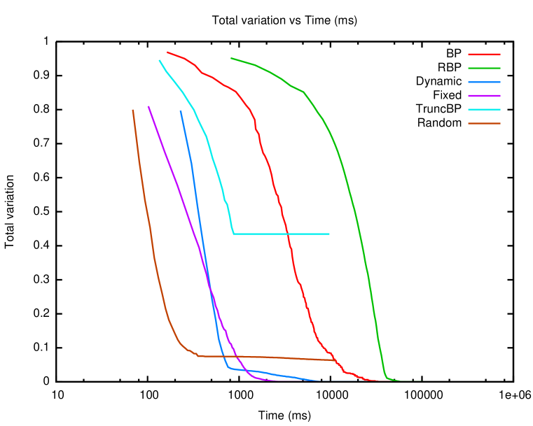
(a) Total Variation Distance

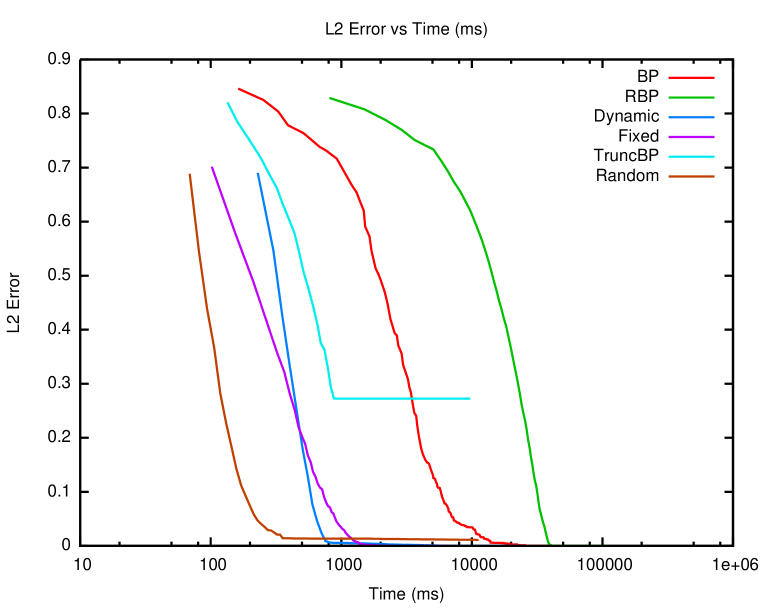
(b) L2 Error

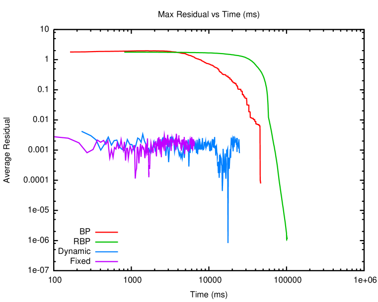
(c) Average Residual in Messages

Figure 1: Runtime Analysis: for 10$\times$10 grid with domain size of $100$, averaged over $10$ runs.

The runtime error for our approaches compared against the marginals obtained by BP at convergence (Figure 1) is significantly better than BP; up to $\bf 12$ times faster to obtain $L_{2}$ error of $10^{-7}$. TruncBP is efficient, however converges to an inaccurate solution, suggesting that prefixed sparsity in domains is not desirable. Similarly, Random is initially fast, since adding any value has a significant impact, however as the selections become crucial, the rate of convergence slows down considerably. Although both Fixed and Dynamic provide desirable trajectories, Fixed is much faster initially due to constant time growth of domains. However as messages and marginals become accurate, the dynamic prioritization that utilizes them eventually overtakes the Fixed approach. To examine the anytime local consistency, we examine the average residuals in Figure 1(c) since low residuals imply a consistent set of marginals for the objective defined over the instantiated domain. Our approaches demonstrate low residuals throughout, while the residuals for existing techniques remain significantly higher (note the log-scale), lowering only near convergence. When the total domain size is varied in Figure 2, we observe that although our proposed approaches are slower on problems with small domains, they obtain significantly higher speedups on larger domains ($\bf 25-40$ times on $250$ labels).

Joint Information Extraction:

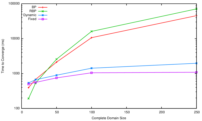
Figure 2: Convergence time for different domains: to $L_{2}<10^{-4}$ over $10$ runs of $5\times 5$ grids.

# Entities 4 6 8 # Vars 16 36 64 # Factors 28 66 120 BP 41,193 91,396 198,374 RBP 54,577 117,850 241,870 Fixed 24,099 26,981 49,227 Dynamic 24,931 36,432 41,371

Figure 3: Joint Information Extraction: Avg time taken (ms) to $L_{2}<0.001$

We also evaluate on the real-world task of joint entity type prediction and relation extraction for the entities that appear in a sentence. The domain sizes for entity types and relations is $42$ and $24$ respectively, resulting in $42,336$ neighbor assignments for joint factors (details omitted due to space). Figure 3 shows the convergence time averaged over $5$ runs. For smaller sentences, sparsity does not help much since BP converges in a few iterations. However, for longer sentences containing many more entities, we observe a significant speedup (up to $\bf 6$ times).

4 Conclusions

In this paper, we describe a novel family of anytime message passing algorithms designed for marginal inference on problems with large domains. The approaches maintain sparse domains, and efficiently compute updates that quickly reach the fixed point of an approximate objective by using dynamic message scheduling. Further, by growing domains based on the gradient of the objective, we improve the approximation iteratively, eventually obtaining the BP marginals.

Appendix A Algorithm

The proposed approach is outlined in Algorithm 1. We initialize the sparse domains using a single value for each variable with the highest priority. The domain priority queue ($Q_{d}$) contains the priorities for the rest of the values of the variables, which remain fixed or are updated depending on the prioritization scheme of choice (Section 2.2). Message passing uses dynamic message prioritization maintained in the message queue $Q_{m}$. Once message passing has converged to obtain locally-consistent marginals (according to some small $\epsilon$), we select another value to add to the domains using one of the value priority schemes, and continue till all the domains are fully-instantiated. If the algorithm is interrupted at any point, we return either the current marginals, or the last converged, locally-consistent marginals. We use a heap-based priority queue for both messages and domain values, in which update and deletion take $O(\log n)$, where $n$ is often smaller than the number of factors and total possible values.

Algorithm 1 Anytime Belief Propagation

1:$\forall x_{i},\mathcal{S}_{i}\leftarrow\{v_{i}\}$ $\triangleright$ where $v_{i}=\displaystyle\operatorname*{arg\,max}_{v_{s}}\pi_{i}(v_{s})$

2:$Q_{d}\oplus\left\langle(i,v_{i}),\pi_{i}(v_{i})\right\rangle$ $\triangleright$ $\forall x_{i},v_{i}\in\mathcal{D}_{i}-\mathcal{S}_{i}$

3:$Q_{m}=\{\}$

4:while $|Q_{d}|>0$ do $\triangleright$ Domains are still partial

5:     GrowDomain($\mathcal{S}$, $Q_{d}$) $\triangleright$ Add a value to a domain, Algorithm 2

6:     ConvergeUsingBP($\mathcal{S}$, $Q_{m}$)$\triangleright$ Converge to a fixed point, Algorithm 3

7:end while$\triangleright$ Converged on full domains

Algorithm 2 Growing by a single value (Section 2.2)

1:procedure GrowDomain($\mathcal{S},Q_{d}$)

2:     $(i,v_{p})\leftarrow Q_{d}.pop$ $\triangleright$ Select value to add

3:     $\mathcal{S}_{i}\leftarrow\mathcal{S}_{i}\cup\{v_{p}\}$ $\triangleright$ Add value to domain

4:     for $f\leftarrow\mathcal{N}(x_{i})$ do

5:         $Q_{m}\oplus\langle f,\pi(f)\rangle$ $\triangleright$ Update msg priority

6:     end for

7:end procedure

Algorithm 3 BP on Sparse Domains (Sect. 2.1, 2.3)

1:procedure ConvergeUsingBP($\mathcal{S},Q_{m}$)

2:     while $max(Q_{m})>\epsilon$ do

3:         $f\leftarrow Q_{m}.pop$ $\triangleright$ Factor with max priority

4:         Pass messages from $f$

5:         for $x_{j}\leftarrow\mathcal{N}_{f};f^{\prime}\leftarrow\mathcal{N}(x_{j})$ do

6:              $Q_{m}\oplus\langle f^{\prime},\pi(f^{\prime})\rangle$ $\triangleright$ Update msg priorities

7:              $Q_{d}\oplus\langle(k,v_{q}),\pi_{k}(v_{k})\rangle$$\triangleright$ $\forall x_{k}\in\mathcal{N}_{f^{\prime}},\forall v_{k}$

8:         end for

9:     end while$\triangleright$ Converged on sparse domains

10:end procedure

References

- Coughlan and Shen [2007] James Coughlan and Huiying Shen. Dynamic quantization for belief propagation in sparse spaces. Computer Vision and Image Understanding, 106:47–58, April 2007. ISSN 1077-3142.
- Coughlan and Ferreira [2002] James M. Coughlan and Sabino J. Ferreira. Finding deformable shapes using loopy belief propagation. In European Conference on Computer Vision (ECCV), pages 453–468, 2002.
- Elidan et al. [2006] G. Elidan, I. McGraw, and D. Koller. Residual belief propagation: Informed scheduling for asynchronous message passing. In Uncertainty in Artificial Intelligence (UAI), 2006.
- Ihler and McAllester [2009] Alexander Ihler and David McAllester. Particle belief propagation. In International Conference on Artificial Intelligence and Statistics (AISTATS), pages 256–263, 2009.
- Ihler et al. [2005] Alexander Ihler, John W. Fisher III, Alan S. Willsky, and Maxwell Chickering. Loopy belief propagation: Convergence and effects of message errors. Journal of Machine Learning Research, 6:905–936, 2005.
- Kschischang et al. [2001] Frank R. Kschischang, Brendan J. Frey, and Hans Andrea Loeliger. Factor graphs and the sum-product algorithm. IEEE Transactions of Information Theory, 47(2):498–519, Feb 2001.
- Murphy et al. [1999] Kevin P. Murphy, Yair Weiss, and Michael I. Jordan. Loopy belief propagation for approximate inference: An empirical study. In Uncertainty in Artificial Intelligence, pages 467–475, 1999.
- Noorshams and Wainwright [2011] Nima Noorshams and Martin J. Wainwright. Stochastic belief propagation: Low-complexity message-passing with guarantees. In Communication, Control, and Computing (Allerton), 2011.
- Shen et al. [2007] Libin Shen, Giorgio Satta, and Aravind Joshi. Guided learning for bidirectional sequence classification. In Association for Computational Linguistics (ACL), 2007.
- Sudderth et al. [2003] E. B. Sudderth, A. T. Ihler, W. T. Freeman, and A. S. Willsky. Nonparametric belief propagation. In Computer Vision and Pattern Recognition (CVPR), 2003.
- Sutton and McCallum [2007] Charles Sutton and Andrew McCallum. Improved dynamic schedules for belief propagation. In Uncertainty in Artificial Intelligence (UAI), 2007.
- Yedidia et al. [2000] J.S. Yedidia, W.T. Freeman, and Y. Weiss. Generalized belief propagation. In Neural Information Processing Systems (NIPS), number 13, pages 689–695, December 2000.
- Yu et al. [2007] Tianli Yu, Ruei-Sung Lin, B. Super, and Bei Tang. Efficient message representations for belief propagation. In International Conference on Computer Vision (ICCV), pages 1 –8, 2007.